Recurrent Neural Networks, Long Short Term Memory

A lot of innovations on NLP have been how to add context into word vectors. One of the common ways of doing it is using Recurrent Neural Networks. The following are the concepts of Recurrent Neural Networks:

• They make use of sequential information.
• They have a memory that captures what have been calculated so far, i.e. what I spoke last will impact what I will speak next.
• RNNs are ideal for text and speech analysis.
• The most commonly used RNNs are LSTMs.

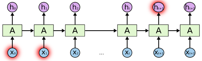
The above is the architecture of Recurrent Neural Networks.

• “A” is one layer of feed-forward neural network.
• If we only look at the right side, it does recurrently to pass through the element of each sequence.
• If we unwrap the left, it will exactly look like the right.

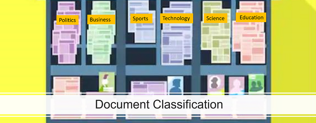
Assuming we are solving document classification problem for a news article data set.

• We input each word, words relate to each other in some ways.
• We make predictions at the end of the article when we see all the words in that article.
• RNNs, by passing input from last output, are able to retain information, and able to leverage all information at the end to make predictions.

• This works well for short sentences, when we deal with a long article, there will be a long term dependency problem.

Therefore, we generally do not use vanilla RNNs, and we use Long Short Term Memory instead. LSTM is a type of RNNs that can solve this long term dependency problem.

In our document classification for news article example, we have this many-to- one relationship. The input are sequences of words, output is one single class or label.

Now we are going to solve a BBC news document classification problem with LSTM using TensorFlow 2.0 & Keras. The data set can be found here.

• First, we import the libraries and make sure our TensorFlow is the right version.

https://medium.com/media/c3ce0e6b10a84a676c3d9de30e90b1fb/href

• Put the hyperparameters at the top like this to make it easier to change and edit.
• We will explain how each hyperparameter works when we get there.

https://medium.com/media/7f3901aa39de489d143a5b733a09ff9c/href

• Define two lists containing articles and labels. In the meantime, we remove stopwords.

https://medium.com/media/78a4697725a3ec5f5861866ffd32cc56/href

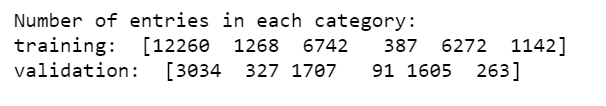
There are 2,225 news articles in the data, we split them into training set and validation set, according to the parameter we set earlier, 80% for training, 20% for validation.

https://medium.com/media/87df8873bbd3b423c283bf3855fcb002/href

Tokenizer does all the heavy lifting for us. In our articles that it was tokenizing, it will take 5,000 most common words. oov_token is to put a special value in when an unseen word is encountered. This means we want <OOV> to be used for words that are not in the word_index. fit_on_text will go through all the text and create dictionary like this:

https://medium.com/media/cef356057de89bd5541b5537c2baeb8b/href

We can see that “<OOV>” is the most common token in our corpus, followed by “said”, followed by “mr” and so on.

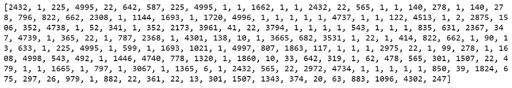
After tokenization, the next step is to turn those tokens into lists of sequence. The following is the 11th article in the training data that has been turned into sequences.

train_sequences = tokenizer.texts_to_sequences(train_articles)
print(train_sequences[10])

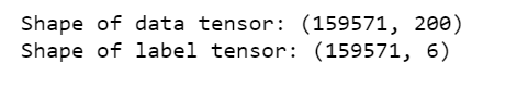
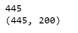
When we train neural networks for NLP, we need sequences to be in the same size, that’s why we use padding. If you look up, our max_length is 200, so we use pad_sequences to make all of our articles the same length which is 200. As a result, you will see that the 1st article was 426 in length, it becomes 200, the 2nd article was 192 in length, it becomes 200, and so on.

train_padded = pad_sequences(train_sequences, maxlen=max_length, padding=padding_type, truncating=trunc_type)

print(len(train_sequences[0]))
print(len(train_padded[0]))

print(len(train_sequences[1]))
print(len(train_padded[1]))

print(len(train_sequences[10]))
print(len(train_padded[10]))

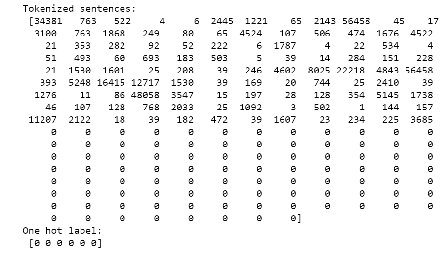
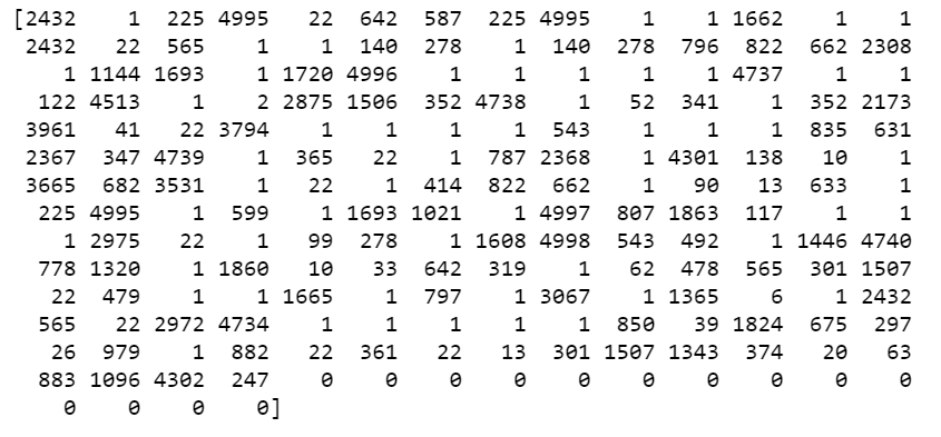
In addition, there is padding_type and truncating_type, there are all post, means for example, for the 11th article, it was 186 in length, we padded to 200, and we padded at the end, that is adding 14 zeros.

print(train_padded[10])

And for the 1st article, it was 426 in length, we truncated to 200, and we truncated at the end as well.

Then we do the same for the validation sequences.

https://medium.com/media/c43e36bb81b9b4fdea972e2ebdb2068c/href

Now we are going to look at the labels. Because our labels are text, so we will tokenize them, when training, labels are expected to be numpy arrays. So we will turn list of labels into numpy arrays like so:

label_tokenizer = Tokenizer()
label_tokenizer.fit_on_texts(labels)

training_label_seq = np.array(label_tokenizer.texts_to_sequences(train_labels))
validation_label_seq = np.array(label_tokenizer.texts_to_sequences(validation_labels))

print(training_label_seq[0])
print(training_label_seq[1])
print(training_label_seq[2])
print(training_label_seq.shape)

print(validation_label_seq[0])
print(validation_label_seq[1])
print(validation_label_seq[2])
print(validation_label_seq.shape)

Before training deep neural network, we should explore what our original article and article after padding look like. Running the following code, we explore the 11th article, we can see that some words become “<OOV>”, because they did not make to the top 5,000.

reverse_word_index = dict([(value, key) for (key, value) in word_index.items()])

def decode_article(text):
return ' '.join([reverse_word_index.get(i, '?') for i in text])
print(decode_article(train_padded[10]))
print('---')
print(train_articles[10])

Now its the time to implement LSTM.

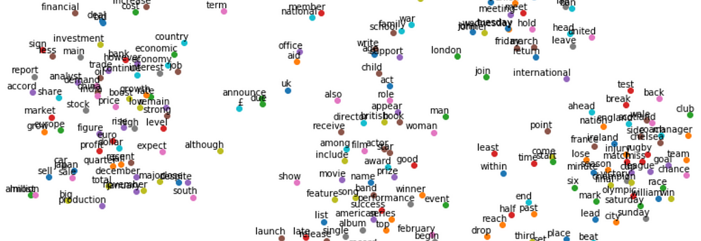
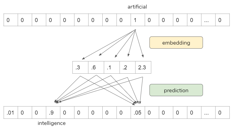
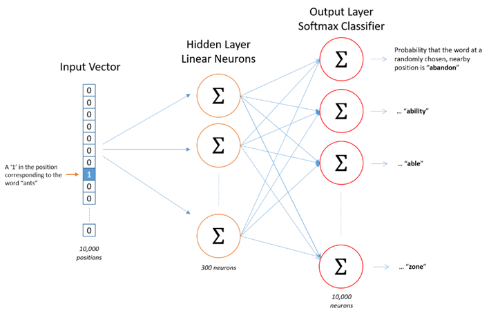
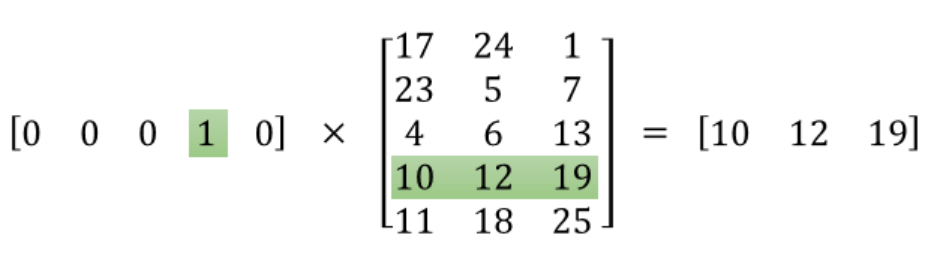
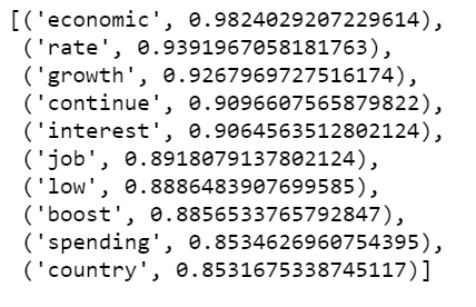
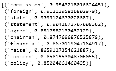
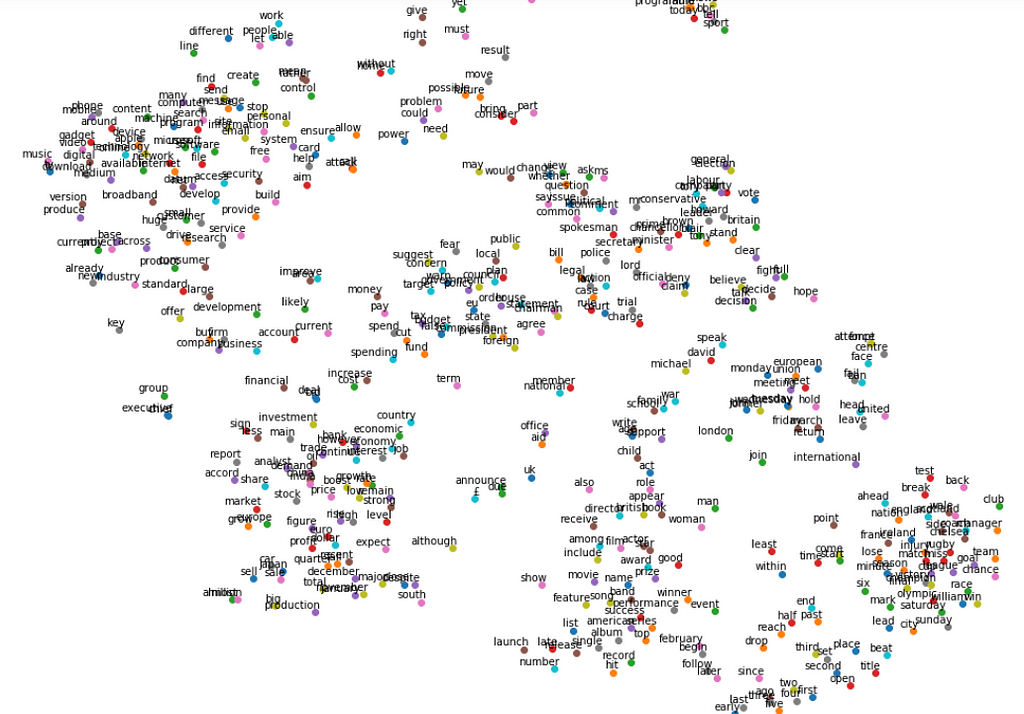
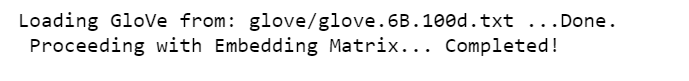
• We build a tf.keras.Sequential model and start with an embedding layer. An embedding layer stores one vector per word. When called, it converts the sequences of word indices into sequences of vectors. After training, words with similar meanings often have the similar vectors.
• The Bidirectional wrapper is used with a LSTM layer, this propagates the input forwards and backwards through the LSTM layer and then concatenates the outputs. This helps LSTM to learn long term dependencies. We then fit it to a dense neural network to do classification.
• We use relu in place of tahn function since they are very good alternatives of each other.
• We add a Dense layer with 6 units and softmax activation. When we have multiple outputs, softmax converts outputs layers into a probability distribution.

https://medium.com/media/928f6aee4451f31480029ddb8efd7cf6/href

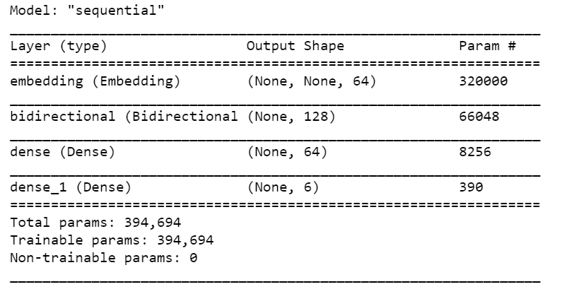
In our model summary, we have our embeddings, our Bidirectional contains LSTM, followed by two dense layers. The output from Bidirectional is 128, because it doubled what we put in LSTM. We can also stack LSTM layer but I found the results worse.

print(set(labels))

We have 5 labels in total, but because we did not one-hot encode labels, we have to use sparse_categorical_crossentropy as loss function, it seems to think 0 is a possible label as well, while the tokenizer object which tokenizes starting with integer 1, instead of integer 0. As a result, the last Dense layer needs outputs for labels 0, 1, 2, 3, 4, 5 although 0 has never been used.

If you want the last Dense layer to be 5, you will need to subtract 1 from the training and validation labels. I decided to leave it as it is.

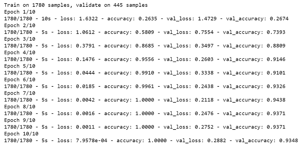
I decided to train 10 epochs, and it is plenty of epochs as you will see.

model.compile(loss='sparse_categorical_crossentropy', optimizer='adam', metrics=['accuracy'])

num_epochs = 10
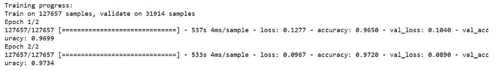
history = model.fit(train_padded, training_label_seq, epochs=num_epochs, validation_data=(validation_padded, validation_label_seq), verbose=2)

def plot_graphs(history, string):
  plt.plot(history.history[string])
  plt.plot(history.history['val_'+string])
  plt.xlabel("Epochs")
  plt.ylabel(string)
  plt.legend([string, 'val_'+string])
  plt.show()

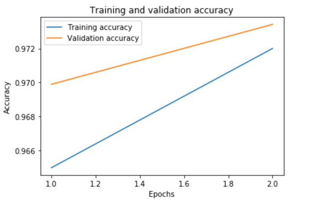
plot_graphs(history, "accuracy")
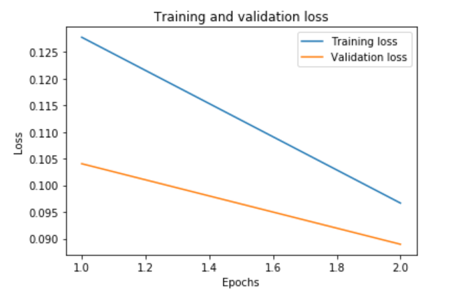
plot_graphs(history, "loss")

We probably only need 3 or 4 epochs. At the end of the training, we can see that there is a little bit overfitting.

In the future posts, we will work on improving the model.

Jupyter notebook can be found on Github. Enjoy the rest of the weekend!

References:

• Coursera | Online Courses From Top Universities. Join for Free
• O’Reilly Strata Data Conference 2019 – New York, New York

Multi Class Text Classification with LSTM using TensorFlow 2.0 was originally published in Towards Data Science on Medium, where people are continuing the conversation by highlighting and responding to this story.

Word embedding, vector space model, Gensim

This post aims to explain the concept of Word2vec and the mathematics behind the concept in an intuitive way while implementing Word2vec embedding using Gensim in Python.

The basic idea of Word2vec is that instead of representing words as one-hot encoding (countvectorizer / tfidfvectorizer) in high dimensional space, we represent words in dense low dimensional space in a way that similar words get similar word vectors, so they are mapped to nearby points.

Word2vec is not deep neural network, it turns text into a numeric form that deep neural network can process as input.

How the word2vec model is trained

• Move through the training corpus with a sliding window: Each word is a prediction problem.
• The objective is to predict the current word using the neighboring words (or vice versa).
• The outcome of the prediction determines whether we adjust the current word vector. Gradually, vectors converge to (hopefully) optimal values.

For example, we can use “artificial” to predict “intelligence”.

However, the prediction itself is not our goal. It is a proxy to learn vector representations so that we can use it for other tasks.

Word2vec Skip-gram Network Architecture

This is one of word2vec models architectures. It is just a simple one hidden layer and one output layer.

The Math

The following is the math behind word2vec embedding. The input layer is the one-hot encoded vectors, so it gets “1” in that word index, “0” everywhere else. When we multiply this input vector by weight matrix, we are actually pulling out one row that is corresponding to that word index. The objective here is to pull out the important row(s), then, we toss the rest.

This is the main mechanics on how word2vec works.

When we use Tensorflow / Keras or Pytorch to do this, they have a special layer for this process called “Embedding layer”. So, we are not going to do math by ourselves, we only need to pass one-hot encoded vectors, the “Embedding layer” does all the dirty works.

Pre-process the text

Now we are going to implement word2vec embedding for a BBC news data set.

• We use Gensim to train word2vec embedding.
• We use NLTK and spaCy to pre-process the text.
• We use t-SNE to visualize high-dimensional data.

https://medium.com/media/18a345d97b747c8f1e6b1da2c040cc4c/href

• We use spaCy for lemmatization.
• Disabling Named Entity Recognition for speed.
• Remove pronouns.

https://medium.com/media/b9cc027d08ca5cc7405113fac1e56640/href

• Now we can have a look top 10 most frequent words.

https://medium.com/media/4323e4c7dfa425044b0a8bf300c310d2/href

Implementing Word2vec embedding in Gensim

• min_count: Minimum number of occurrences of a word in the corpus to be included in the model. The higher the number, the less words we have in our corpus.
• window: The maximum distance between the current and predicted word within a sentence.
• size: The dimensionality of the feature vectors.
• workers: I know my system is having 4 cores.
• model.build_vocab: Prepare the model vocabulary.
• model.train: Train word vectors.
• model.init_sims(): When we do not plan to train the model any further, we use this line of code to make the model more memory-efficient.

https://medium.com/media/a1f70ba732dbe1f8d3df7e3c9827fe81/href

Explore the model

• Find the most similar words for “economy”

w2v_model.wv.most_similar(positive=['economy'])

• Find the most similar words for “president”

w2v_model.wv.most_similar(positive=['president'])

• How similar are these two words to each other?

w2v_model.wv.similarity('company', 'business')

Please note, the above results could change if we change min_count. For example, if we set min_count=100, we will have more words to work with, some of them may be more similar to the target words than the above results; If we set min_count=300, some of the above results may disappear.

• We Use t-SNE to represent high-dimensional data in a lower-dimensional space.

https://medium.com/media/dcc0ba898b2e4d11c9a1503608b690dc/href

• It is obvious that some words are close to each other, such as “team”, “goal”, “injury”, “olympic” and so on. And those words tend to be used in the sport related news articles.
• Other words that cluster together such as “film”, “actor”, “award”, “prize” and so on, they are likely to be used in the news articles that talk about entertainment.
• Again. How the plot looks like pretty much depends on how we set min_count.

The Jupyter notebook can be found on Github. Enjoy the rest of the week.

Reference: https://learning.oreilly.com/videos/oreilly-strata-data/9781492050681/9781492050681-video327451?autoplay=false

Understanding Word2vec Embedding in Practice was originally published in Towards Data Science on Medium, where people are continuing the conversation by highlighting and responding to this story.

Yes

Thank you for the great idea. I will try it as soon as I get around to.

Identify similar records, Sparse matrix multiplication

Online world is full of duplicate listings. In particular, if you are an online travel agency, and you accept different suppliers that provide you information for the same property.

Sometimes the duplicate records are obvious that makes you think: How is it possible?

Another time, the two records look like they are duplicates, but we were not sure.

Or, if you work for a company that has significant amount of data about companies or customers, but because the data comes from different source systems, in which are often written in different ways. Then you will have to deal with duplicate records.

The Data

I think the best data set is to use my own. Using the Seattle Hotel data set that I created a while ago. I removed hotel description feature, kept hotel name and address features, and added duplicate records purposely, and the data set can be found here.

An example on how two hotels are duplicates:

https://medium.com/media/9f825cf1034adde99e086628cbd06561/href

The most common way of duplication is how the street address is input. Some are using the abbreviations and others are not. For the human reader it is obvious that the above two listings are the same thing. And we will write a program to determine and remove the duplicate records and keep one only.

TF-IDF + N-gram

• We will use name and address for input features.
• We all familiar with tfidf and n-gram methods.
• The result we get is a sparse matrix that each row is a document(name_address), each column is a n-gram. The tfidf score is computed for each n-gram in each document.

https://medium.com/media/a1c7cfdffab34416823d13fb25ff8c93/href

Sparse_dot_topn

I discovered an excellent library that developed by ING Wholesale Banking, sparse_dot_topn which stores only the top N highest matches for each item, and we can choose to show the top similarities above a threshold.

It claims that it provides faster way to perform a sparse matrix multiplication followed by top-n multiplication result selection.

The function takes the following things as input:

• A and B: two CSR matrix
• ntop: n top results
• lower_bound: a threshold that the element of A*B must greater than output

The output is a resulting matrix.

https://medium.com/media/ab9ab56ff91a20aec471569f9879d406/href

After running the function. The matrix only stores the top 5 most similar hotels.

The following code unpacks the resulting sparse matrix, the result is a table where each hotel will match to every hotel in the data(include itself), and cosine similarity score is computed for each pair.

https://medium.com/media/4586d0709b6d121c5000fe965da68916/href

We are only interested in the top matches except itself. So we are going to visual examine the resulting table sort by similarity scores, in which we determine a threshold a pair is the same property.

matches_df[matches_df['similarity'] < 0.99999].sort_values(by=['similarity'], ascending=False).head(30)

I decided my safe bet is to remove any pairs where the similarity score is higher than or equal to 0.50.

matches_df[matches_df['similarity'] < 0.50].right_side.nunique()

After that, we now have 152 properties left. If you remember, in our original data set, we did have 152 properties.

Jupyter notebook and the dataset can be found on Github. Have a productive week!

De-duplicate the Duplicate Records from Scratch was originally published in Towards Data Science on Medium, where people are continuing the conversation by highlighting and responding to this story.

How to effectively and creatively pre-process text data

A few months ago, we built a content based recommender system using a relative clean text data set. Because I collected the hotel descriptions my self, I made sure that the descriptions were useful for the goals we were going to accomplish. However, the real-world text data is never clean and there are different pre-processing ways and steps for different goals.

Topic modeling in NLP is rarely my final goal in an analysis, I use it often to either explore data or as a tool to make my final model more accurate. Let me show you what I meant.

The Data

We are still using the Seattle Hotel description data set I collected earlier, and I made it a bit more messier this time. We are going to skip all the EDA processes and I want to make recommendations as quickly as possible.

If you have read my previous post, I am sure you understand the following code script. Yes, we are looking for top 5 most similar hotels with “Hilton Garden Inn Seattle Downtown” (except itself), according to hotel description texts.

Make Recommendations

https://medium.com/media/aafe45c62a3f78bdd069868868db2b66/href

Our model returns the above 5 hotels and thinks they are top 5 most similar hotels to “Hilton Garden Inn Seattle Downtown”. I am sure you don’t agree, neither do I. Let’s say why the model thinks they are similar by looking at these descriptions.

df.loc['Hilton Garden Inn Seattle Downtown'].desc

df.loc["Mildred's Bed and Breakfast"].desc

df.loc["Seattle Airport Marriott"].desc

Found anything interesting? Yes, there are indeed somethings in common in these three hotel descriptions, they all have the same check in and check out time, and they all have the similar smoking policies. But are they important? Can we declare two hotels are similar just because they are all “non-smoking”? Of course not, these are not important characteristics and we shouldn’t measure similarity in vector space of these texts.

We need to find a way to safely remove these texts programmatically, while not removing any other useful characteristics.

Topic modeling comes to our rescue. But before that, we need to wrangle the data to make it in the right shape.

• Split each description into sentences. Hilton Garden Seattle Downtown’s entire description will be split into 7 sentences.

https://medium.com/media/57f6877b6638b27c9e142fa3a5bb7c63/href

Topic Modeling

• We are going to build topic model for all the sentences together. I decided to have 40 topics after several experiments.

https://medium.com/media/0478e76d0041ce7510ce5092c27e42b9/href

Not too bad, there were not too much overlapping.

• To understand better, you may want to investigate top 20 words in each topic.

https://medium.com/media/3667d3da9af7aee9b9e721ffd1ae853b/href

We shall have 40 topics, and each topic shows 20 keywords. Its very hard to print out the entire table, I will only show a small part of it.

By staring at the table, we can guess that at least topic 12 should be one of the topics we would like to dismiss, because it contains several words that meaningless for our purpose.

In the following code scripts, we:

• Create document-topic matrix.
• Create a data frame where each document is a row, and each column is a topic.
• The weight of each topic is assigned to each document.
• The last column is the dominant topic for that document, in which it carries the most weight.
• When we merge this data frame to the previous sentence data frame. We are able to find the the weight of each topic in every sentence, and the dominant topic for each sentence.

https://medium.com/media/4d76caf58479fd78fe5beaae6256fabd/href

• Now we can visually examine dominant topics assignment of each sentence for “Hilton Garden Inn Seattle Downtown”.

df_sent_topic.loc[df_sent_topic['name'] == 'Hilton Garden Inn Seattle Downtown'][['sentence', 'dominant_topic']]

• By staring at the above table, my assumption is that if a sentence’s dominant topic is topic 4 or topic 12, that sentence is likely to be useless.
• Let’s see a few more example sentences that have topic 4 or topic 12 as their dominant topic.

df_sent_topic.loc[df_sent_topic['dominant_topic'] == 4][['sentence', 'dominant_topic']].sample(20)

df_sent_topic.loc[df_sent_topic['dominant_topic'] == 12][['sentence', 'dominant_topic']].sample(10)

• After reviewing the above two tables, I decided to remove all the sentences that have topic 4 or topic 12 as their dominant topic.

print('There are', len(df_sent_topic.loc[df_sent_topic['dominant_topic'] == 4]), 'sentences that belong to topic 4 and we will remove')
print('There are', len(df_sent_topic.loc[df_sent_topic['dominant_topic'] == 12]), 'sentences that belong to topic 12 and we will remove')

df_sent_topic_clean = df_sent_topic.drop(df_sent_topic[(df_sent_topic.dominant_topic == 4) | (df_sent_topic.dominant_topic == 12)].index)

• Next, we will join the clean sentence together in to a descriptions. That is, making it back to one description per hotel.

df_description = df_sent_topic_clean[['sentence','name']]
df_description = df_description.groupby('name')['sentence'].agg(lambda col: ' '.join(col)).reset_index()

• Let’s see what left for our “Hilton Garden Inn Seattle Downtown”

df_description['sentence'][45]

There is only one sentence left and it is about the location of the hotel and this is what I had expected.

Make Recommendations

Using the same cosine similarity measurement, we are going to find the top 5 most similar hotels with “Hilton Garden Inn Seattle Downtown” (except itself), according to the cleaned hotel description texts.

https://medium.com/media/2338ec051f9d736f4062aa769eace360/href

Nice! Our method worked!

Jupyter notebook can be found on Github. Have a great weekend!

Correct.

Thank you for your feedback. I did not try this time.

Deep learning, text classification, NLP

This article shows how to use a simple LSTM and one of the pre-trained GloVe files to create a strong baseline for the toxic comments classification problem.

The article consist of 4 main sections:

• Preparing the data
• Implementing a simple LSTM (RNN) model
• Training the model
• Evaluating the model

The Data

In the following steps, we will set the key model parameters and split the data.

• “MAX_NB_WORDS” sets the maximum number of words to consider as features for tokenizer.
• “MAX_SEQUENCE_LENGTH” cuts off texts after this number of words (among the MAX_NB_WORDS most common words).
• “VALIDATION_SPLIT” sets a portion of data for validation and not used in training.
• “EMBEDDING_DIM” defines the size of the “vector space”.
• “GLOVE_DIR” defines the GloVe file directory.
• Split the data into the texts and the labels.

https://medium.com/media/e404f87284057d710e0e0f3967897354/href

Text Pre-processing

In the following step, we remove stopwords, punctuation and make everything lowercase.

https://medium.com/media/eadbd6070963e87f8225525edc19beff/href

Have a look a sample data.

print('Sample data:', texts[1], y[1])

• We create a tokenizer, configured to only take into account the MAX_NB_WORDS most common words.
• We build the word index.
• We can recover the word index that was computed.

tokenizer = Tokenizer(num_words=MAX_NB_WORDS)
tokenizer.fit_on_texts(texts)
sequences = tokenizer.texts_to_sequences(texts)
word_index = tokenizer.word_index
print('Vocabulary size:', len(word_index))

• Turns the lists of integers into a 2D integer tensor of shape (samples, maxlen)
• Pad after each sequence.

data = pad_sequences(sequences, padding = 'post', maxlen = MAX_SEQUENCE_LENGTH)

print('Shape of data tensor:', data.shape)
print('Shape of label tensor:', y.shape)

• Shuffle the data.

indices = np.arange(data.shape[0])
np.random.shuffle(indices)
data = data[indices]
labels = y[indices]

Create the train-validation split.

num_validation_samples = int(VALIDATION_SPLIT*data.shape[0])
x_train = data[: -num_validation_samples]
y_train = labels[: -num_validation_samples]
x_val = data[-num_validation_samples: ]
y_val = labels[-num_validation_samples: ]

print('Number of entries in each category:')
print('training: ', y_train.sum(axis=0))
print('validation: ', y_val.sum(axis=0))

This is what the data looks like:

print('Tokenized sentences: n', data[10])
print('One hot label: n', labels[10])

Create the model

• We will use pre-trained GloVe vectors from Stanford to create an index of words mapped to known embeddings, by parsing the data dump of pre-trained embeddings.
• Then load word embeddings into an embeddings_index

https://medium.com/media/4a58a99c42bc4a3760b0155be6d63f59/href

• Create the embedding layers.
• Specifies the maximum input length to the Embedding layer.
• Make use of the output from the previous embedding layer which outputs a 3-D tensor into the LSTM layer.
• Use a Global Max Pooling layer to to reshape the 3D tensor into a 2D one.
• We set the dropout layer to drop out 10% of the nodes.
• We define the Dense layer to produce a output dimension of 50.
• We feed the output into a Dropout layer again.
• Finally, we feed the output into a “Sigmoid” layer.

https://medium.com/media/6d48566a561c43069f9da57f9ad9e800/href

Its time to Compile the model into a static graph for training.

• Define the inputs, outputs and configure the learning process.
• Set the model to optimize our loss function using “Adam” optimizer, define the loss function to be “binary_crossentropy” .

model = Model(sequence_input, preds)
model.compile(loss = 'binary_crossentropy',
             optimizer='adam',
             metrics = ['accuracy'])

Training

• Feed in a list of 32 padded, indexed sentence for each batch. The validation set will be used to assess whether the model has overfitted.
• The model will run for 2 epochs, because even 2 epochs is enough to overfit.

print('Training progress:')
history = model.fit(x_train, y_train, epochs = 2, batch_size=32, validation_data=(x_val, y_val))

Evaluate the model

loss = history.history['loss']
val_loss = history.history['val_loss']

epochs = range(1, len(loss)+1)

plt.plot(epochs, loss, label='Training loss')
plt.plot(epochs, val_loss, label='Validation loss')
plt.title('Training and validation loss')
plt.xlabel('Epochs')
plt.ylabel('Loss')
plt.legend()
plt.show();

accuracy = history.history['accuracy']
val_accuracy = history.history['val_accuracy']

plt.plot(epochs, accuracy, label='Training accuracy')
plt.plot(epochs, val_accuracy, label='Validation accuracy')
plt.title('Training and validation accuracy')
plt.ylabel('Accuracy')
plt.xlabel('Epochs')
plt.legend()
plt.show();

Jupyter notebook can be found on Github. Happy Monday!

Classify Toxic Online Comments with LSTM and GloVe was originally published in Towards Data Science on Medium, where people are continuing the conversation by highlighting and responding to this story.

Collaborative Filtering is a technique widely used by recommender systems when you have a decent size of user — item data. It makes recommendations based on the content preferences of similar users.

Therefore, collaborative filtering is not a suitable model to deal with cold start problem, in which it cannot draw any inference for users or items about which it has not yet gathered sufficient information.

But once you have relative large user — item interaction data, then collaborative filtering is the most widely used recommendation approach. And we are going to learn how to build a collaborative filtering recommender system using TensorFlow.

The Data

We are again using booking crossing dataset that can be found here. The data pre-processing steps does the following:

• Merge user, rating and book data.
• Remove unused columns.
• Filtering books that have had at least 25 ratings.
• Filtering users that have given at least 20 ratings. Remember, collaborative filtering algorithms often require users’ active participation.

https://medium.com/media/defd12f7c924869652fef81d9795e6c6/href

So, our final dataset contains 3,192 users for 5,850 books. And each user has given at least 20 ratings and each book has received at least 25 ratings. If you do not have a GPU, this would be a good size.

The collaborative filtering approach focuses on finding users who have given similar ratings to the same books, thus creating a link between users, to whom will be suggested books that were reviewed in a positive way. In this way, we look for associations between users, not between books. Therefore, collaborative filtering relies only on observed user behavior to make recommendations — no profile data or content data is necessary.

Our technique will be based on the following observations:

• Users who rate books in a similar manner share one or more hidden preferences.
• Users with shared preferences are likely to give ratings in the same way to the same books.

The Process in TensorFlow

First, we will normalize the rating feature.

scaler = MinMaxScaler()
combined['Book-Rating'] = combined['Book-Rating'].values.astype(float)
rating_scaled = pd.DataFrame(scaler.fit_transform(combined['Book-Rating'].values.reshape(-1,1)))
combined['Book-Rating'] = rating_scaled

Then, build user, book matrix with three features:

combined = combined.drop_duplicates(['User-ID', 'Book-Title'])
user_book_matrix = combined.pivot(index='User-ID', columns='Book-Title', values='Book-Rating')
user_book_matrix.fillna(0, inplace=True)

users = user_book_matrix.index.tolist()
books = user_book_matrix.columns.tolist()

user_book_matrix = user_book_matrix.as_matrix()

tf.placeholder only available in v1, so I have to work around like so:

import tensorflow.compat.v1 as tf
tf.disable_v2_behavior()

In the following code scrips

• We set up some network parameters, such as the dimension of each hidden layer.
• We will initialize the TensorFlow placeholder.
• Weights and biases are randomly initialized.
• The following code are taken from the book: Python Machine Learning Cook Book — Second Edition

https://medium.com/media/b9d3ea77cc85bc45921c16d0d53e2ffb/href

Now, we can build the encoder and decoder model.

https://medium.com/media/7eefae55b835e0f730c1a2f1dd21c16d/href

Now, we construct the model and the predictions

encoder_op = encoder(X)
decoder_op = decoder(encoder_op)

y_pred = decoder_op

y_true = X

In the following code, we define loss function and optimizer, and minimize the squared error, and define the evaluation metrics.

loss = tf.losses.mean_squared_error(y_true, y_pred)
optimizer = tf.train.RMSPropOptimizer(0.03).minimize(loss)
eval_x = tf.placeholder(tf.int32, )
eval_y = tf.placeholder(tf.int32, )
pre, pre_op = tf.metrics.precision(labels=eval_x, predictions=eval_y)

Because TensorFlow uses computational graphs for its operations, placeholders and variables must be initialized before they have values. So in the following code, we initialize the variables, then create an empty data frame to store the result table, which will be top 10 recommendations for every user.

init = tf.global_variables_initializer()
local_init = tf.local_variables_initializer()
pred_data = pd.DataFrame()

We can finally start training our model.

• We split training data into batches, and we feed the network with them.
• We train our model with vectors of user ratings, each vector represents a user and each column a book, and entries are ratings that the user gave to books.
• After a few trials, I discovered that training model for 100 epochs with a batch size of 35 would be consuming enough memories. This means that the entire training set will feed our neural network 100 times, every time using 35 users.
• At the end, we must make sure to remove user’s ratings in the training set. That is, we must not recommend books to a user in which he (or she) has already rated.

https://medium.com/media/fcd7f1ee4eb1aa50cc9c45ecd402244c/href

Finally, let’s see how our model works. I randomly selected a user, to see what books we should recommended to him (or her).

top_ten_ranked.loc[top_ten_ranked['User-ID'] == 278582]

The above are the top 10 results for this user, sorted by the normalized predicted ratings.

Let’s see what books he (or she) has rated, sorted by ratings.

book_rating.loc[book_rating['User-ID'] == 278582].sort_values(by=['Book-Rating'], ascending=False)

The types of the books this user liked are: historical mystery novel, thriller and suspense novel, science and fiction novel, fantasy novel and so on.

The top 10 results for this user are: murder fantasy novel, mystery thriller novel and so on.

The results were not disappointing.

The Jupyter notebook can be found on Github. Happy Friday!

References:

Python Machine Learning Cook Book — Second Edition

https://cloud.google.com/solutions/machine-learning/recommendation-system-tensorflow-overview

Building A Collaborative Filtering Recommender System with TensorFlow was originally published in Towards Data Science on Medium, where people are continuing the conversation by highlighting and responding to this story.