
Blog

Learn About Our Meetup

5000+ Members

MEETUPS

LEARN, CONNECT, SHARE

Join our meetup, learn, connect, share, and get to know your Toronto AI community. 

JOB POSTINGS

INDEED POSTINGS

Browse through the latest deep learning, ai, machine learning postings from Indeed for the GTA.

CONTACT

CONNECT WITH US

Are you looking to sponsor space, be a speaker, or volunteer, feel free to give us a shout.

Category: Amazon

Cinnamon AI saves 70% on ML model training costs with Amazon SageMaker Managed Spot Training

Developers are constantly training and re-training machine learning (ML) models so they can continuously improve model predictions. Depending on the dataset size, model training jobs can take anywhere from a few minutes to multiple hours or days. ML development can be a complex, expensive, and iterative process. Being compute intensive, keeping compute costs low for ML development is vital and a key enabler to achieving scale.

Amazon SageMaker is a fully managed service to build, train, tune, and deploy ML models at scale. Amazon SageMaker Managed Spot Training enables you to save up to 90% in training costs by using Amazon EC2 Spot Instances for training.

EC2 Spot Instances are a great way to optimize compute costs for ML training workloads, they use spare Amazon EC2 capacity which is available for up to a 90% discount over On-Demand Instances. When there is a spike in requests for a particular On-Demand instance type in a specific availability zone (AZ), AWS can reclaim the Spot Instances with a two-minute notification.

This post describes how Cinnamon AI reduced their ML training costs by 70% and increased the number of daily training jobs by 40% without increasing their budgets by using Amazon SageMaker Managed Spot Training.

Amazon SageMaker Managed Spot Training

Managed Spot Training uses EC2 Spot Instances to run training jobs instead of On-Demand Instances. With Managed Spot Training, Amazon SageMaker manages the Spot capacity and handles interruptions. In case of a Spot interruption, Managed Spot Training pauses the training job and reliably resumes as Spot capacity becomes available. As a result, Managed Spot Training is best suited for model training jobs with flexible starting times and run durations. You can configure your training job to use checkpoints. When enabled, Amazon SageMaker copies checkpoint data from a local path to Amazon S3 and resumes interrupted training jobs from the last checkpoint instead of restarting. Managed Spot Training eliminates the need for you to build additional tooling to poll for Spot capacity or manage interruptions. You can use Managed Spot Training when training models built using the popular ML frameworks, Amazon SageMaker built-in algorithms, and custom-built models.

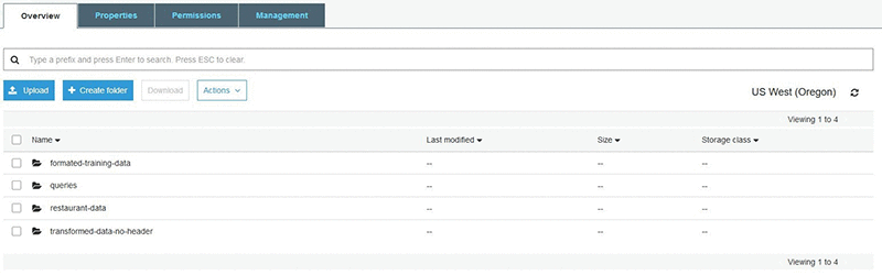
To enable the feature, choose Enable managed spot training on the Amazon SageMaker console. See the following screenshot.

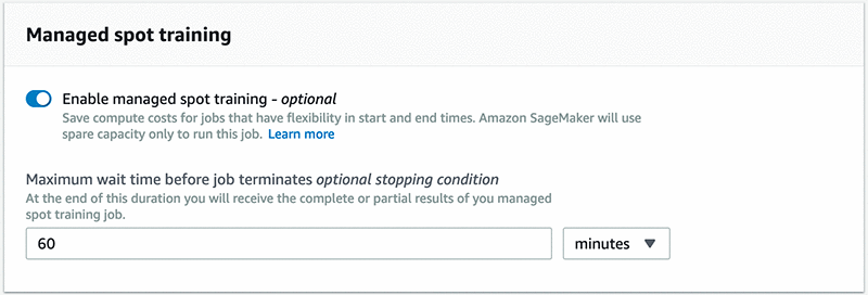
If you are using Amazon SageMaker SDK, set train_use_spot_instances to true in the Estimator constructor. You can also specify a stopping condition that controls how long Amazon SageMaker waits for Spot Instances to become available.

Cinnamon AI saves 70% on model training costs

With the massive opportunity that cognitive and artificial intelligence (AI) systems present, many companies are developing AI-powered products to build intelligent services. One such innovator is Cinnamon AI, a Japan-based startup with a mission to “extend human potential by eliminating repetitive tasks” through their AI service offerings.

Cinnamon AI’s flagship product, Flax Scanner, is a document reader that uses natural language processing (NLP) algorithms to automate data extraction from unstructured business documents such as invoices, receipts, insurance claims, and financial statements. It converts these documents into database-ready files. The goal is to eliminate the need for humans to read such documents to extract the required data, thus saving businesses millions of hours in time and reducing their operational costs. This service also works on hand-written documents and with Japanese characters.

Cinnamon AI has also developed two other ML-powered services called Rossa Voice and Aurora. Rossa Voice is a high-precision, real-time voice recognition service that has applications around voice fraud detection and to transcribe records at call centers. And Aurora is a service that automatically extracts necessary information from long sentences in documents. You can use this service to find important information from specifications and contract documents.

Cinnamon AI had a goal to reduce their ML development costs, so they decided to consolidate their disparate development environments into a single platform and then continuously optimize on costs. They chose AWS to develop their ML services on because of AWS’s breadth of services, cost effective pricing options, granular security controls, and technical support. As a first step, Cinnamon AI migrated all their ML workloads from on-premises environments and other cloud providers onto AWS. Next, the team optimized their EC2 usage and started using Amazon SageMaker to train their ML models. More recently, they started using the Managed Spot Training feature to use Spot Instances for training, which helped them optimize their cost profile significantly.

“The Managed Spot Training feature of Amazon SageMaker has had a profound impact on our AWS cost savings. Our AWS EC2 costs reduced by up to 70% after using Managed Spot Training,” said Tetsuya Saito, General Manager of Infrastructure and Information Security Office at Cinnamon AI. “In addition, Managed Spot Training does not require complicated methods and can be used simply from the SageMaker SDK.”

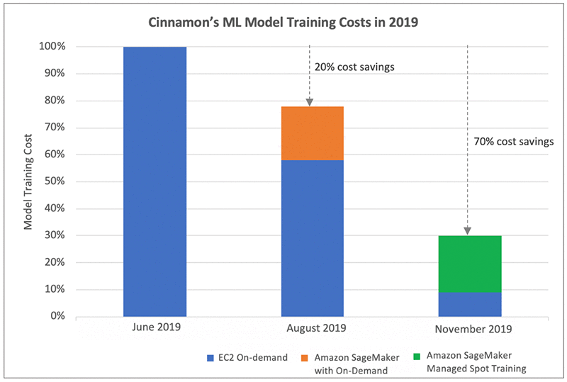
The following graph shows Cinnamon AI’s model training cost savings journey over six months. In June 2019, after moving their ML workloads onto AWS, they started using EC2 On-Demand Instances for model training. You can use this as a point of reference from a training cost perspective. Over the next few months, they optimized their EC2 On-Demand usage mainly through instance right sizing and using GPU instances (P2, P3) for large training jobs. They also adopted Amazon SageMaker for model training with On-Demand Instances and reduced their training costs by approximately 20%. Furthermore, they saw substantial cost savings of 70% by using Managed Spot Training to use Spot Instances for model training in November 2019. Their cost optimization effort also resulted in their ability to increase the number of daily model training jobs by 40%, while maintaining a reduced cost profile.

Cinnamon AI’s Model Development Environment

As Cinnamon AI is developing multiple ML-powered products and services, their data types vary based on the application and include 2D images, audio, and text with dataset sizes ranging from 100 MB to 40 GB. They predominantly use custom deep learning models and their frameworks of choice are TensorFlow, PyTorch, and Keras. They use GPU instances for time-consuming neural network training jobs, with run times ranging from a few hours to days, and use CPU instances for smaller model training experiments.

The following architecture depicts Cinnamon AI’s ML environment and workflow at a high level.

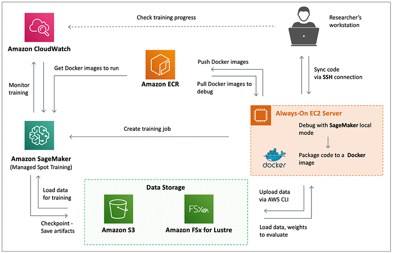
The AI researchers develop code on their workstations and then synchronize it to a shared always-on EC2 server (On-Demand instance). This instance is used to call Amazon SageMaker local mode to run, test, and debug their scripts and models on small datasets. After the executed code is tested, it is packaged into a Docker image and stored in Amazon ECR. This enables researchers to share their work across teams and to pull the required Docker image from ECR on their respective Amazon SageMaker training instances. Also, on the EC2 server, the researchers can use the Amazon SageMaker Python SDK to initialize an Amazon SageMaker Estimator and then launch training jobs in Amazon SageMaker.

Almost all of Cinnamon AI’s training jobs run on Spot Instances in Amazon SageMaker via Managed Spot Training, with checkpointing enabled to save the state of the models. Amazon SageMaker saves the checkpoints to Amazon S3 while the training is in progress, and they can use them to resume training in events of Spot interruptions. In addition to S3, Cinnamon AI uses Amazon FSx for Lustre to feed data to Amazon SageMaker for training ML models. Using Amazon FSx for Lustre has reduced the data loading time to the SageMaker training instance compared to directly loading the data from S3. They can access the data in S3 and Amazon FSx for Lustre by both the EC2 instance and the SageMaker training instance. Amazon SageMaker publishes training metrics to Amazon CloudWatch, which Cinnamon AI researchers use to monitor their training jobs.

Conclusion

Managed Spot Training is a great way to optimize model training costs for jobs with flexible starting times and run durations. The Cinnamon AI team has successfully taken advantage of the cost-saving strategies with Amazon SageMaker and has increased the number of daily experiments and reduced training costs by 70%. If you are not using Spot Instances for model training, try out Managed Spot Training. For more information, see Managed Spot Training: Save Up to 90% On Your Amazon SageMaker Training Jobs. You can get started with Amazon SageMaker here.


About the Authors

Sundar Ranganathan is a Principal Business Development Manager on the EC2 team focusing on EC2 Spot for AI/ML in addition to Big Data, Containers, and DevOps workloads. His experience includes leadership roles in product management and product development at NetApp, Micron Technology, Qualcomm, and Mentor Graphics.


Yoshitaka Haribara, Ph.D., is a Startup Solutions Architect in Japan focusing on machine learning workloads. He helped Cinnamon AI to migrate their workload on to Amazon SageMaker.


Additional contributions by by Shoko Utsunomiya, a Senior Solution Architect at AWS.

Building machine learning workflows with AWS Data Exchange and Amazon SageMaker

Thanks to cloud services such as Amazon SageMaker and AWS Data Exchange, machine learning (ML) is now easier than ever. This post explains how to build a model that predicts restaurant grades of NYC restaurants using AWS Data Exchange and Amazon SageMaker. We use a dataset of 23,372 restaurant inspection grades and scores from AWS Data Exchange alongside Amazon SageMaker to train and deploy a model using the Linear Learner Algorithm.

Background

ML workflows are an iterative process that require many decisions to be made such as whether or not training data is needed, what attributes to capture, what algorithms to use, and where to deploy a trained model. All of these decisions effect the outcome of a learning system. Once a problem is defined, you must choose from four distinct types of learning systems. Some learning systems depend entirely on training data where others require no training data at all, but rather a well-defined environment and action space. When an algorithm relies on training data, the quality and sensitivity of the final model depends heavily on the characteristics of the training set. It is here that many enter the tedious loop of trying to find the right balance of features that will result in a well-balanced and accurate model. An overview of each learning system can be seen below:

  1. Supervised – In supervised learning the training set includes labels so the algorithm knows the correct label given a set of attributes. For example, the attributes could be the color and weight of a fish where the label is the type of fish. Eventually the model learns how to assign the correct or most probable label. A typical supervised learning task is classification, which is the task of assigning inputs such as text or images to one of several predefined categories. Examples include detecting spam email messages based upon the message header and content, categorizing cells as malignant or benign based upon the results of MRI scans, and classifying galaxies based upon their shapes (Tan et al. 2006). The algorithms used in this category typically consist of k-nearest neighbors, linear regression, logistic regression, support vector machines, and neural networks.
  2. Unsupervised – Unsupervised learning uses algorithms that discover relationships in unlabeled data. The algorithms must explore the data and find the relationships based on the known features. Some of the common algorithms used within unsupervised learning include clustering (K-means, DBSCAN, and hierarchical cluster analysis) where you are grouping similar data points, anomaly detection where you are trying to find outliers, as well as association rule learning where you are trying to discover the correlation between features (Aurélien 2019). In practice, this could be seen by clustering cities based on crime rates to find out which cities are alike or clustering products at a grocery store based on customer age to discover patterns.
  3. Semi-supervised – Semi-supervised learning uses training data that consists of both labeled and unlabeled data. The algorithms are often a combination of both unsupervised and supervised algorithms. If you were to have a dataset with unlabeled data the first step would be to label the data. Once the dataset has been labeled, you can train your algorithm with traditional supervised learning techniques to map your features to known labels. Photo-hosting services often use this workflow by using your skills to label an unknown face. Once the face is known another algorithm can scan all your photos to identify the now known face.
  4. Reinforcement – Reinforcement learning (RL) differs from the previous learning systems because it doesn’t have to learn from training data. Instead, the model learns from its own experience in the context of a well-defined environment. The learning system is called an agent and that agent can observe the environment, select and perform actions based on a policy, and get rewards in return. The agent eventually learns to maximize its reward over time based on its previous experience. For more information or to get some clarity about RL, see the documentation on Amazon SageMaker RL.

Steps to build the restaurant grade prediction model

When beginning an ML project, it is important to think about the whole process and not just the final product. In this project, we go through the following steps:

  1. Define the problem you want to solve. In this case, we want to make better informed choices on where to eat in NYC based on cleanliness.
  2. Find a dataset to train your model. We want a dataset that contains restaurant inspection grades and scores in NYC.
  3. Review the data. We want to make sure the data we need is present and that there is enough to train the model.
  4. Prepare and clean the dataset for training in Amazon SageMaker. We want to only include the needed data such as borough and food category and ensure the correct format is used.
  5. Select a model for multi-class classification. In our case we are training with the Linear Learner Algorithm.
  6. Deploy the model to Amazon SageMaker. With the model deployed to Amazon SageMaker we can invoke the endpoint to get predictions.

Data is the foundation of ML; the quality of the final model depends on the quality of the data used for training. In our workflow, half of the steps are related to data collection and preparation. This theme can be seen in most ML projects and is often the most challenging part. Additionally, you have to think about the characteristics of your data to prevent an overly sensitive or perhaps a not sensitive enough model. Furthermore, not all data is internal. You may have to use either free or paid third-party data to enrich internal datasets and improve the quality of the model, but finding, licensing, and consuming this third-party data has been a challenge for years. Fortunately, you now have AWS Data Exchange.

Using AWS Data Exchange

AWS Data Exchange can simplify the data collection process by making it easy to find, subscribe to, and use third-party data in the cloud. You can browse over 1,500 data products from more than 90 qualified data providers in the AWS Marketplace. Previously, there was the need for access to more data to drive your analytics, train ML models, and make data-driven decisions, but now with AWS Data Exchange, you have all of that in one place. For more information, see AWS Data Exchange – Find, Subscribe To, and Use Data Products.

AWS Data Exchange makes it easy to get started with ML. You can jump-start your projects using one or a combination of the hundreds of datasets available. You can also enrich your internal data with external third-party data. All the datasets are available using a single cloud-native API that delivers your data directly to Amazon S3, which we will see in our workflow. This saves you and your team valuable time and resources, which you can now use for more value-added activities. With this combination, you can take data from AWS Data Exchange and feed it into Amazon SageMaker to train and deploy your models.

Using Amazon SageMaker

Amazon SageMaker is a fully managed service that enables you to quickly and easily build, train, and deploy ML models. You can take the NYC restaurant data from AWS Data Exchange and use the features of Amazon SageMaker to train and deploy a model. You will be using fully managed instances that run Jupyter notebooks to explore and preprocess the training data. These notebooks are pre-loaded with CUDA and cuDNN drivers for popular deep learning platforms, Anaconda packages, and libraries for TensorFlow, Apache MXNet, and PyTorch.

You will also be using supervised algorithms such as the linear learner algorithm to train the model. Finally, the model is deployed to an Amazon SageMaker endpoint to begin servicing requests and predicting restaurant grades. By combining the power of AWS Data Exchange with Amazon SageMaker, you have a robust set of tools to start solving the most challenging ML problems, and you are perfectly positioned to start building multi-class classifiers.

Solution overview

The solution in this post produces a multi-class classifier that can predict the grade of restaurants in New York City based on borough and food category. The following diagram shows the complete architecture.

First, take the data from AWS Data Exchange and place it into an S3 bucket. Point an AWS Glue crawler at it to create a Data Catalog of the data. With the Data Catalog in place, use Amazon Athena to query, clean, and format the data for training. When the data has transformed, load the training set back into S3. Finally, create a Jupyter notebook in Amazon SageMaker to train, deploy, and invoke your predictor.

Storing data in S3

Getting training data is often a time-consuming and challenging part of an ML project. In this case, you need to make sure that you can actually find a large enough dataset that has inspection information for restaurants in NYC, and that it contains the right attributes. Fortunately, with AWS Data Exchange you can start searching the product catalog for data. In this case, you are interested in the quality of restaurants in New York City, so enter New York Restaurant Data in the search bar and filter for free datasets. There is a product from Intellect Design Arena, Inc. offered for free, titled NY City Restaurant Data with inspection grade & score (Trial).

After you subscribe to the dataset, you need to find a way to expose the data to other AWS services. To accomplish this, export the data to S3 by choosing your subscription, your dataset, and a revision, and exporting to S3. When the data is in S3, you can download the file and look at the data to see what features are captured. The following screenshot shows the revision page which allows you to export your data using the “Export to Amazon S3” button.

You can now download the file and look at the contents to understand how much data there is and what attributes are captured. For this example, you are only concerned with three attributes: the borough (labeled BORO), cuisine description, and the grade. A new file is created that only contains the data relevant to this use case and loaded back into S3. With the data in S3, other AWS services can quickly and securely access the data. The following screenshot captures an example of what your S3 bucket might look like once your folders and data have been loaded.

Create a Data Catalog with AWS Glue crawlers

The data in its current form is not formatted correctly for training in Amazon SageMaker, so you need to build an Extract, Transform, Load (ETL) pipeline to get this dataset into the proper format. Later in the pipeline, you use Athena to query this data and generate a formatted training set, but currently the data is just a CSV file in a bucket and we need a way to interact with the data. You can use AWS Glue crawlers to scan your data and generate a Data Catalog that enables Athena to query the data within S3. For more information, see Defining Crawlers. After the AWS Glue crawler runs, you now have a Data Catalog that Athena can use to query data. The details of your data are captured and can be seen by clicking on the newly created Data Catalog. The following screenshot shows the Data Catalog interface, which contains all the information pertaining to your data.

Querying data in Athena and creating a training set

Now that you have a dataset in S3 and the data catalog from the AWS Glue crawler, you can use Athena to start querying and formatting the data. You can use the integrated query editor to generate SQL queries that allow you to explore and transform the data. For this example, you created a SQL query to generate the following training set. This is to simplify the training process because you are moving from text-based attributes to numerically based attributes. When using the linear learner algorithm for multi-class classification, it is a requirement that the class labels be numerical values from 0 to N-1, where N is the number of possible classes. After you run the query in Athena, you can download the results and place the new dataset into S3. You are now ready to begin training a model in Amazon SageMaker. See the following code:

SELECT boro_data.id AS "boro_label",
         category_data.id AS "cat_label",
         class_label
FROM data
LEFT JOIN boro_data
    ON data.boro = boro_data.boro
LEFT JOIN category_data
    ON data.cuisine_description = category_data.cuisine_description

The SQL query creates a numerical representation of the attributes and class labels, which can be seen in the following table.

boro_label cat_label class_label
1 5 8 0
2 5 8 0
3 5 8 0
4 5 8 0
5 5 8 0
6 5 8 0
7 5 8 0
8 5 8 0
9 5 8 0
10 5 8 0
11 5 8 0
12 5 8 0
13 5 8 0
14 5 8 0
15 5 8 0

Training and deploying a model in Amazon SageMaker

Now that you have clean data, you will use Amazon SageMaker to build, train, and deploy your model. First, create a Jupyter notebook in Amazon SageMaker to start writing and executing your code. You then import your data from S3 into your Jupyter notebook environment and proceed to train the model. To train the model, use the linear learner algorithm that comes included in Amazon SageMaker. The linear learner algorithm provides a solution for both classification and regression problems, but in this post, you are focusing on classification. The following Python code shows the steps to load, format, and train your model:

import numpy as np
import pandas as pd
import boto3
from sklearn.model_selection import train_test_split
import sagemaker

#declare bucket name and file name
bucket = 'qs-demo-bgf'
prefix = 'transformed-data-no-header/'
fileName = 'transformed_data_no_header.csv'

#load data 
s3 = boto3.resource('s3')

KEY = prefix+fileName
print(KEY)

#load data into jupyter environment
s3.Bucket(bucket).download_file(KEY,'transformed_data_no_header.csv')

data = pd.read_csv('transformed_data_no_header.csv',dtype='float32').values

data_features, data_labels = data[:, :2], data[:, 2]
np.random.seed(0)
train_features, test_features, train_labels, test_labels = train_test_split(
    data_features, data_labels, test_size=0.2)

# further split the test set into validation and test sets
val_features, test_features, val_labels, test_labels = train_test_split(
    test_features, test_labels, test_size=0.5)

# instantiate the LinearLearner estimator object
multiclass_estimator = sagemaker.LinearLearner(role=sagemaker.get_execution_role(),
                                               train_instance_count=1,
                                               train_instance_type='ml.m4.xlarge',
                                               predictor_type='multiclass_classifier',
                                               num_classes=3)
# wrap data in RecordSet objects
train_records = multiclass_estimator.record_set(train_features, train_labels, channel='train')
val_records = multiclass_estimator.record_set(val_features, val_labels, channel='validation')
test_records = multiclass_estimator.record_set(test_features, test_labels, channel='test')

# start a training job
multiclass_estimator.fit([train_records, val_records, test_records])

After the training job is complete, you can deploy the model onto an instance. This provides you with an endpoint that listens for prediction requests. See the following Python code:

# deploy a model hosting endpoint
multiclass_predictor = multiclass_estimator.deploy(initial_instance_count=1, instance_type='ml.m4.xlarge')

Invoking an Amazon SageMaker endpoint

Now that you have a trained model deployed, you are ready to start invoking the endpoint to get predictions. The endpoint provides a score for each class type and a predicted label based on the highest score. You now have an endpoint that you can integrate into your application. The following Python code is an example of invoking the endpoint in an Amazon SageMaker notebook:

import json 
import boto3 
client = boto3.client('runtime.sagemaker')

#define a dictionary to map text to numerical values
area = {
    "Queens":1.0,
    "Staten Island":2.0,
    "Brooklyn":3.0,
    "Bronx":4.0,
    "Manhattan":5.0
}

cat = {
    "Hotdogs/Pretzels":1.0,
    "Donuts":2.0,
    "Bangladeshi":3.0,
    "Caribbean":4.0,
    "Chicken":5.0
}

#assign features to pass to endpoint
location = area["Manhattan"]
category = cat["Hotdogs/Pretzels"]

values = str(location)+','+str(category)

#get response from endpoint
response = client.invoke_endpoint(EndpointName='linear-learner-2019-11-04-01-57-20-572',
                                  ContentType='text/csv',
                                  Body=values)

#parse the results
result = json.loads(response['Body'].read().decode())

predict = result['predictions'][0]
print(predict)

grade = predict['predicted_label']

if(grade==0.0):
    letter = "A"
elif(grade==1.0):
    letter = "B"
else:
    letter = "C"

#get readable prediction
print("Restaurant Grade: "+letter)

After the endpoint is invoked, a response is provided and formatted into a readable prediction. See the following code:

{'score': [0.9355735182762146, 0.0486408956348896, 0.01578556001186371], 'predicted_label': 0.0}

Restaurant Grade: A

Cleaning up

To prevent any ongoing billing, you should clean up your resources. Start with AWS Data Exchange. If you subscribed to the dataset used in this example, set the subscription to terminate at the end of the one-month trial period. Delete any S3 buckets that are storing data used in this example. Delete the AWS Glue Data Catalog that you created as a result of the AWS Glue crawler. Also, delete your Amazon SageMaker notebook instance and the endpoint that you created from deploying your model.

Summary

This post provided an example workflow that uses AWS Data Exchange and Amazon SageMaker to build, train, and deploy a multi-class classifier. You can use AWS Data Exchange to jump-start your ML projects with third-party data, and use Amazon SageMaker to create solutions for your ML tasks with built-in tools and algorithms. If you are in the early stages of your ML project or are looking for a way to improve your already existing datasets, check out AWS Data Exchange. You could save yourself hours of data wrangling.

References

  • Géron Aurélien. Hands-on Machine Learning with Scikit-Learn, Keras, and TensorFlow: Concepts, Tools, and Techniques to Build Intelligent Systems. OReilly, 2019.
  • Tan, Pang-Ning, et al. Introduction to Data Mining. Pearson, 2006.

About the author

Ben Fields is a Solutions Architect for Strategic Accounts based out of Seattle, Washington. His interests and experience include AI/ML, containers, and big data. You can often find him out climbing at the nearest climbing gym, playing ice hockey at the closest rink, or enjoying the warmth of home with a good game.


Building a custom classifier using Amazon Comprehend

Amazon Comprehend is a natural language processing (NLP) service that uses machine learning (ML) to find insights and relationships in texts. Amazon Comprehend identifies the language of the text; extracts key phrases, places, people, brands, or events; and understands how positive or negative the text is. For more information about everything Amazon Comprehend can do, see Amazon Comprehend Features.

You may need out-of-the-box NLP capabilities tied to your needs without having to lead a research phase. This would allow you to recognize entity types and perform document classifications that are unique to your business, such as recognizing industry-specific terms and triaging customer feedback into different categories.

Amazon Comprehend is a perfect match for these use cases. In November 2018, Amazon Comprehend added the ability for you to train it to recognize custom entities and perform custom classification. For more information, see Build Your Own Natural Language Models on AWS (no ML experience required).

This post demonstrates how to build a custom text classifier that can assign a specific label to a given text. No prior ML knowledge is required.

About this blog post
Time to complete 1 hour for the reduced dataset ; 2 hours for the full dataset
Cost to complete ~ $50 for the reduced dataset ; ~ $150 for the full dataset
These include training, inference and model management, see Amazon Comprehend pricing for more details.
Learning level Advanced (300)
AWS services Amazon Comprehend
Amazon S3
AWS Cloud9

Prerequisites

To complete this walkthrough, you need an AWS account and access to create resources in AWS IAM, Amazon S3, Amazon Comprehend, and AWS Cloud9 within that account.

This post uses the Yahoo answers corpus cited in the paper Text Understanding from Scratch by Xiang Zhang and Yann LeCun. This dataset is available on the AWS Open Data Registry.

You can also use your own dataset. It is recommended that you train your model with up to 1,000 training documents for each label, and that when you select your labels, suggest labels that are clear and don’t overlap in meaning. For more information, see Training a Custom Classifier.

Solution overview

The walkthrough includes the following steps:

  1. Preparing your environment
  2. Creating an S3 bucket
  3. Setting up IAM
  4. Preparing data
  5. Training the custom classifier
  6. Gathering results

For more information about how to build a custom entity recognizer to extract information such as people and organization names, locations, time expressions, numerical values from a document, see Build a custom entity recognizer using Amazon Comprehend.

Preparing your environment

In this post, you use the AWS CLI as much as possible to speed up the experiment.

AWS Cloud9 is a cloud-based integrated development environment (IDE) that lets you write, run, and debug your code with a browser. It includes a code editor, debugger, and terminal. AWS Cloud9 comes pre-packaged with essential tools for popular programming languages and the AWS CLI pre-installed, so you don’t need to install files or configure your laptop for this workshop.

Your AWS Cloud9 environment has access to the same AWS resources as the user with which you logged in to the AWS Management Console.

To prepare your environment, complete the following steps:

  1. On the console, under Services, choose AWS Cloud9.
  2. Choose Create environment.
  3. For Name, enter CustomClassifier.
  4. Choose Next step.
  5. Under Environment settings, change the instance type to t2.large.
  6. Leave other settings at their defaults.
  7. Choose Next step.
  8. Review the environment settings and choose Create environment.

It can take up to a few minutes for your environment to be provisioned and prepared. When the environment is ready, your IDE opens to a welcome screen, which contains a terminal prompt.

You can run AWS CLI commands in this prompt the same as you would on your local computer.

  1. To verify that your user is logged in, enter the following command:
Admin:~/environment $ aws sts get-caller-identity

You get the following output which indicates your account and user information:

{
    "Account": "123456789012",
    "UserId": "AKIAI53HQ7LSLEXAMPLE",
    "Arn": "arn:aws:iam::123456789012:user/Colin"
}
  1. Record the account ID to use in the next step.

Keep your AWS Cloud9 IDE opened in a tab throughout this walkthrough.

Creating an S3 bucket

Use the account ID from the previous step to create a globally unique bucket name, such as 123456789012-customclassifier. Enter the following command in your AWS Cloud9 terminal prompt:

Admin:~/environment $ aws s3api create-bucket --acl private --bucket '123456789012-comprehend' --region us-east-1

The output shows the name of the bucket you created:

{
    "Location": "/123456789012-comprehend"
}

Setting up IAM

To authorize Amazon Comprehend to perform bucket reads and writes during the training or during the inference, you must grant Amazon Comprehend access to the S3 bucket that you created. You are creating a data access role in your account to trust the Amazon Comprehend service principal.

To set up IAM, complete the following steps:

  1. On the console, under Services, choose IAM.
  2. Choose Roles.
  3. Choose Create role.
  4. Select AWS service as the type of trusted entity.
  5. Choose Comprehend as the service that uses this role.
  6. Choose Next: Permissions.

The Policy named ComprehendDataAccessRolePolicy is automatically attached.

  1. Choose Next: Review
  2. For Role name, enter ComprehendBucketAccessRole.
  3. Choose Create role.
  4. Record the Role ARN.

You use this ARN when you launch the training of your custom classifier.

Preparing data

In this step, you download the corpus and prepare the data to match Amazon Comprehend’s expected formats for both training and inference. This post provides a script to help you achieve the data preparation for your dataset.

Alternatively, for even more convenience, you can download the prepared data by entering the following two command lines:

Admin:~/environment $ aws s3 cp s3://aws-ml-blog/artifacts/comprehend-custom-classification/comprehend-test.csv . 

Admin:~/environment $ aws s3 cp s3://aws-ml-blog/artifacts/comprehend-custom-classification/comprehend-train.csv .

If you follow the preceding step, skip the next steps and go directly to the upload part at the end of this section.

If you want to go through the dataset preparation for this walkthrough, or if you are using your own data follow the next steps:

Enter the following command in your AWS Cloud9 terminal prompt to download it from the AWS Open Data registry:

Admin:~/environment $ aws s3 cp s3://fast-ai-nlp/yahoo_answers_csv.tgz .

You see a progress bar and then the following output:

download: s3://fast-ai-nlp/yahoo_answers_csv.tgz to ./yahoo_answers_csv.tgz

Uncompress it with the following command:

Admin:~/environment $ tar xvzf yahoo_answers_csv.tgz

You should delete the archive because you are limited in available space in your AWS Cloud9 environment. Use the following command:

Admin:~/environment $ rm -f yahoo_answers_csv.tgz

You get a folder yahoo_answers_csv, which contains the following four files:

  • classes.txt
  • readme.txt
  • test.csv
  • train.csv

The files train.csv and test.csv contain the training samples as comma-separated values. There are four columns in them, corresponding to class index (1 to 10), question title, question content, and best answer. The text fields are escaped using double quotes (“), and any internal double quote is escaped by two double quotes (“”). New lines are escaped by a backslash followed with an “n” character, that is “n”.

The following code is the overview of file content:

"5","why doesn't an optical mouse work on a glass table?","or even on some surfaces?","Optical mice use an LED
"6","What is the best off-road motorcycle trail ?","long-distance trail throughout CA","i hear that the mojave
"3","What is Trans Fat? How to reduce that?","I heard that tras fat is bad for the body.  Why is that? Where ca
"7","How many planes Fedex has?","I heard that it is the largest airline in the world","according to the www.fe
"7","In the san francisco bay area, does it make sense to rent or buy ?","the prices of rent and the price of b

The file classes.txt contains the available labels.

The train.csv file contains 1,400,000 lines and test.csv contains 60,000 lines. Amazon Comprehend uses between 10–20% of the documents submitted for training to test the custom classifier.

The following command indicates that the data is evenly distributed:

Admin:~/environment $ awk -F '","' '{print $1}'  yahoo_answers_csv/train.csv | sort | uniq -c

You should train your model with up to 1,000 training documents for each label and no more than 1,000,000 documents.

With 20% of 1,000,000 used for testing, that is still plenty of data to train your custom classifier.

Use a shortened version of train.csv to train your custom Amazon Comprehend model, and use test.csv to perform your validation and see how well your custom model performs.

For training, the file format must conform to the following requirements:

  • File must contain one label and one text per line – 2 columns
  • No header
  • Format UTF-8, carriage return “n”.

Labels must be uppercase, can be multi-token, have white space, consist of multiple words connected by underscores or hyphens, or may even contain a comma, as long as it is correctly escaped.

The following table contains the formatted labels proposed for the training.

Index Original For training
1 Society & Culture SOCIETY_AND_CULTURE
2 Science & Mathematics SCIENCE_AND_MATHEMATICS
3 Health HEALTH
4 Education & Reference EDUCATION_AND_REFERENCE
5 Computers & Internet COMPUTERS_AND_INTERNET
6 Sports SPORTS
7 Business & Finance BUSINESS_AND_FINANCE
8 Entertainment & Music ENTERTAINMENT_AND_MUSIC
9 Family & Relationships FAMILY_AND_RELATIONSHIPS
10 Politics & Government POLITICS_AND_GOVERNMENT

When you want your custom Amazon Comprehend model to determine which label corresponds to a given text in an asynchronous way, the file format must conform to the following requirements:

  • File must contain one text per line
  • No header
  • Format UTF-8, carriage return “n”.

This post includes a script to speed up the data preparation. Enter the following command to copy the script to your local AWS Cloud9 environment:

Admin:~/environment $ aws s3 cp s3://aws-ml-blog/artifacts/comprehend-custom-classification/prepare_data.py .

To launch data preparation, enter the following commands:

Admin:~/environment $ sudo pip-3.6 install pandas tqdm
Admin:~/environment $ python3 prepare_data.py

This script is tied to the Yahoo corpus and uses the pandas library to format the training and testing datasets to match your Amazon Comprehend expectations. You may adapt it to your own dataset or change the number of items in the training dataset and validation dataset.

When the script is finished (it should run for approximately 11 minutes on a t2.large instance for the full dataset, and in under 5 minutes for the reduced dataset), you have the following new files in your environment:

  • comprehend-train.csv
  • comprehend-test.csv

Upload the prepared data (either the one you downloaded or the one you prepared) to the bucket you created with the following commands:

Admin:~/environment $ aws s3 cp comprehend-train.csv s3://123456789012-comprehend/

Admin:~/environment $ aws s3 cp comprehend-test.csv s3://123456789012-comprehend/

Training the custom classifier

You are ready to launch the custom text classifier training. Enter the following command, and replace the role ARN and bucket name with your own:

Admin:~/environment $ aws comprehend create-document-classifier --document-classifier-name "yahoo-answers" --data-access-role-arn arn:aws:iam:: 123456789012:role/ComprehendBucketAccessRole --input-data-config S3Uri=s3://123456789012-comprehend/comprehend-train.csv --output-data-config S3Uri=s3://123456789012-comprehend/TrainingOutput/ --language-code en

You get the following output that names the custom classifier ARN:

{
    "DocumentClassifierArn": "arn:aws:comprehend:us-east-1:123456789012:document-classifier/yahoo-answers"
}

It is an asynchronous call. You can then track the training progress with the following command:

Admin:~/environment $ aws comprehend describe-document-classifier --document-classifier-arn arn:aws:comprehend:us-east-1:123456789012:document-classifier/yahoo-answers

You get the following output:

{
    "DocumentClassifierProperties": {
        "DocumentClassifierArn": "arn:aws:comprehend:us-east-1: 123456789012:document-classifier/yahoo-answers",
        "Status": "TRAINING", 
        "LanguageCode": "en", 
        "DataAccessRoleArn": "arn:aws:iam:: 123456789012:role/ComprehendBucketAccessRole", 
        "InputDataConfig": {
            "S3Uri": "s3://123456789012-comprehend/comprehend-train.csv"
        },
        "SubmitTime": 1571657958.503, 
        "OutputDataConfig": {
            "S3Uri": "s3://123456789012-comprehend/TrainingOutput/123456789012-CLR-b205910479f3a195124bea9b70c4e2a9/output/output.tar.gz"
        }
    }
}

When the training is finished, you get the following output:

{
    "DocumentClassifierProperties": {
        "DocumentClassifierArn": "arn:aws:comprehend:us-east-1: 123456789012:document-classifier/yahoo-answers",
        "Status": "TRAINED", 
        "LanguageCode": "en", 
        "DataAccessRoleArn": "arn:aws:iam:: 123456789012:role/ComprehendBucketAccessRole", 
        "InputDataConfig": {
            "S3Uri": "s3://123456789012-comprehend/comprehend-train.csv"
        },
        "OutputDataConfig": {
            "S3Uri": "s3://123456789012-comprehend/TrainingOutput/123456789012-CLR-b205910479f3a195124bea9b70c4e2a9/output/output.tar.gz"
        },
        "SubmitTime": 1571657958.503,
        "EndTime": 1571661250.482,
        "TrainingStartTime": 1571658140.277
        "TrainingEndTime": 1571661207.915,
        "ClassifierMetadata": {
            "NumberOfLabels": 10,
            "NumberOfTrainedDocuments": 989873,
            "NumberOfTestDocuments": 10000,
            "EvaluationMetrics": {
                "Accuracy": 0.7235,
                "Precision": 0.722,
                "Recall": 0.7235,
                "F1Score": 0.7219
            }
        },
    }
}

The training duration may vary; in this case, the training took approximately one hour for the full dataset (20 minutes for the reduced dataset).

The output for the training on the full dataset shows that your model has a recall of 0.72—in other words, it correctly identifies 72% of given labels.

The following screenshot shows the view from the console (Comprehend > Custom Classification > yahoo-answers).

Gathering results

You can now launch an inference job to test how the classifier performs. Enter the following commands:

Admin:~/environment $ aws comprehend start-document-classification-job --document-classifier-arn arn:aws:comprehend:us-east-1:123456789012:document-classifier/yahoo-answers --input-data-config S3Uri=s3://123456789012-comprehend/comprehend-test.csv,InputFormat=ONE_DOC_PER_LINE --output-data-config S3Uri=s3://123456789012-comprehend/InferenceOutput/ --data-access-role-arn arn:aws:iam::123456789012:role/ComprehendBucketAccessRole

You get the following output:

{
    "JobStatus": "SUBMITTED", 
    "JobId": "cd5a6ee7f490a353e33f50d866d0317a"
}

Just as you did for the training progress tracking, because the inference is asynchronous, you can check the progress of the newly launched job with the following command:

Admin:~/environment $ aws comprehend describe-document-classification-job --job-id cd5a6ee7f490a353e33f50d866d0317a

You get the following output:

{
    "DocumentClassificationJobProperties": {
        "InputDataConfig": {
            "S3Uri": "s3://123456789012-comprehend/comprehend-test.csv", 
            "InputFormat": "ONE_DOC_PER_LINE"
        }, 
        "DataAccessRoleArn": "arn:aws:iam:: 123456789012:role/ComprehendBucketAccessRole", 
        "DocumentClassifierArn": "arn:aws:comprehend:us-east-1: 123456789012:document-classifier/yahoo-answers", 
        "JobStatus": "IN_PROGRESS", 
        "JobId": "cd5a6ee7f490a353e33f50d866d0317a", 
        "SubmitTime": 1571663022.503, 
        "OutputDataConfig": {
            "S3Uri": "s3://123456789012-comprehend/InferenceOutput/123456789012-CLN-cd5a6ee7f490a353e33f50d866d0317a/output/output.tar.gz"
        }
    }
}

When it is completed, JobStatus changes to COMPLETED. This takes approximately a few minutes to complete.

Download the results using OutputDataConfig.S3Uri path with the following command:

Admin:~/environment $ aws s3 cp s3://123456789012-comprehend/InferenceOutput/123456789012-CLN-cd5a6ee7f490a353e33f50d866d0317a/output/output.tar.gz .

When you uncompress the output (tar xvzf output.tar.gz), you get a .jsonl file. Each line represents the result of the requested classification for the corresponding line of the document you submitted.

For example, the following code is one line from the predictions:

{"File": "comprehend-test.csv", "Line": "9", "Classes": [{"Name": "ENTERTAINMENT_AND_MUSIC", "Score": 0.9685}, {"Name": "EDUCATION_AND_REFERENCE", "Score": 0.0159}, {"Name": "BUSINESS_AND_FINANCE", "Score": 0.0102}]}

This means that your custom model predicted with a 96.8% confidence score that the following text was related to the “Entertainment and music” label.

"What was the first Disney animated character to appear in color? n Donald Duck was the first major Disney character to appear in color, in his debut cartoon, "The Wise Little Hen" in 1934.nnFYI: Mickey Mouse made his color debut in the 1935 'toon, "The Band Concert," and the first color 'toon from Disney was "Flowers and Trees," in 1932."

Each line of results also provides the second and third possible labels. You might use these different scores to build your application upon applying each label with a score superior to 40% or changing the model if no single score is above 70%.

Summary

With the full dataset for training and validation, in less than two hours, you used Amazon Comprehend to learn 10 custom categories—and achieved a 72% recall on the test—and to apply that custom model to 60,000 documents.

Try custom categories now from the Amazon Comprehend console. For more information, see Custom Classification. You can discover other Amazon Comprehend features and get inspiration from other AWS blog posts about how to use Amazon Comprehend beyond classification.

Amazon Comprehend can help you power your application with NLP capabilities in almost no time. Happy experimentation!


About the Author

Hervé Nivon is a Solutions Architect who helps startup customers grow their business on AWS. Before joining AWS, Hervé was the CTO of a company generating business insights for enterprises from commercial unmanned aerial vehicle imagery. Hervé has also served as a consultant at Accenture.


Using Amazon Lex Conversation logs to monitor and improve interactions

As a product owner for a conversational interface, understanding and improving the user experience without the corresponding visibility or telemetry can feel like driving a car blindfolded. It is important to understand how users are interacting with your bot so that you can continuously improve the bot based on past interactions. You can gain these actionable insights by monitoring bot conversations. To capture user input, you could write custom logic in your application, but building and managing additional code and associated infrastructure is both cumbersome and time-consuming. You would also need to make sure that the custom logic does not increase the latency for end-users.

We are excited to announce Conversation logs for Amazon Lex, which enables you to natively save interactions with your bot. You can configure logging text input to Amazon CloudWatch Logs and audio input to Amazon S3. In addition to the user input and bot responses, the logs contain information such as matched intent and missed utterances. To protect sensitive data captured as slot values, you can enable slot obfuscation to mask those values for logging.

You can use Conversation logs to track utterances that were not mapped to any configured intent. These missed utterances allow you to improve the bot design. Now that conversation transcripts for the entire session are available, you can better analyze the conversation flow, improve conversational design, and increase user engagement.

This post demonstrates how to enable conversation logs, obfuscate sensitive slots, and set up advanced monitoring capabilities for your bot.

Building a bot

This post uses the following conversation to model a bot for an auto loan:

User: I’d like to check the outstanding balance on my car loan.
Agent: Sure, can you provide me your account number?
User: It is 12345678.
Agent: Can you please confirm the last four digits of your SSN for verification?
User: 1234
Agent: Thank you for the information. The balance on your car loan for account 12345678 is $12,345.
User: Ok thanks.

Build the Amazon Lex bot AutoLoanBot (download) with the following intents:

  • ApplyLoan – Elicits necessary information, such as name and SSN, and creates a new request.
  • PayInstallment – Captures the user’s account number, the last four digits of the user’s SSN, and payment information, and processes the monthly installment.
  • CheckBalance – Elicits the user’s account number and the last four digits of their SSN and provides the outstanding balance.
  • Fallback – Captures any input that the bot cannot process by the configured intents.

Create an alias Prod and publish a version of the bot using this alias.

Enabling Conversation logs

You can create Conversation logs for both text and audio.

Text logs

Before configuring Conversation text logs, create a new log group car-loan-bot-text-logs in CloudWatch Logs. As an optional step, you can encrypt the text logs. For more information, see Encrypt Log Data in CloudWatch Logs Using AWS KMS. Additionally, create the IAM role LexCarLoanBotRole to provide write permissions to the car-loan-bot-text-logs log group.

To set up text logs for a bot alias, complete the following steps:

  1. On the Amazon Lex console, choose the AutoLoanBot.
  2. Choose Settings.
  3. Choose Conversation logs.
  4. Choose the Settings gear icon that corresponds to the Prod
  5. Under Log type, choose Text logs.
  6. For Log group name, select car-loan-bot-text-logs from the dropdown list.
  7. For IAM role, select LexCarLoanBotRole from the dropdown list.
  8. Choose Save.

Audio logs

Before configuring Conversation audio logs, create the S3 bucket car-loan-bot-audio-logs. As an optional step, you can encrypt the audio logs with a KMS customer managed CMK. To do so, create the new KMS key car-loan-bot-audio-logs-kms-key. Additionally, create the IAM role LexCarLoanBotRole to provide write permissions to the car-loan-bot-audio-logs S3 bucket and access permissions to car-loan-bot-audio-logs-kms-key.

To enable audio logging, complete the following steps:

  1. On the Amazon Lex console, choose the AutoLoanBot.
  2. Choose Settings.
  3. Choose Conversation logs.
  4. Choose the Settings gear icon that corresponds to the Prod
  5. For Log type, select Audio logs.
  6. For S3 bucket, select car-loan-bot-audio-logs from the dropdown menu.
  7. For KMS key, select car-loan-bot-audio-logs-kms-key from the dropdown menu.
  8. For IAM role, select LexCarLoanBotRole from the dropdown menu.
  9. Choose Save.

You can modify or disable Conversation logs settings for an alias by choosing the Settings gear icon. If you are enabling both text and audio logs, the LexCarLoanBotRole must have write permissions to car-loan-bot-text-logs log group and car-loan-bot-audio-logs S3 bucket.

Marking sensitive slots as obfuscated

To protect sensitive data captured as slot values, you can enable slot obfuscation to mask those values for logging. To mask the SSN or last four digits of the SSN in the Conversation logs, mark them as obfuscated in Applyloan, PayInstallment, and CheckBalance. Complete the following steps:

  1. On the Amazon Lex console, choose AutoLoanBot.
  2. Under Intents, choose CheckBalance.
  3. Choose the Settings gear icon corresponding to the SSNFourDigit slot.

The popup SSNFourDigit settings appears.

  1. For Slot Obfuscation section, choose Store as {SSNFourDigit}.
  2. Choose Save.
  3. Choose Build.
  4. Choose Publish using the Prod alias.

Your bot is now ready to deploy.

Reviewing Conversation logs data

After you enable Conversation logs for the alias Prod, the user input is saved in CloudWatch Logs log group in the following format, with the SSN slot obfuscated:

{
    "messageVersion": "1.0",
    "botName": "AutoLoanBot",
    "botAlias": "Prod",
    "botVersion": "2",
    "inputTranscript": "Yes",
    "botResponse": "Thank you, your application for a car loan of $50000 has been submitted.",
    "intent": "ApplyLoan",
    "slots": {
        "DateOfBirth": "1990-01-01",
        "LoanAmount": "50000",
        "Address": "1234 First Avenue",
        "FirstName": "John",
        "PhoneNumber": "1234567890",
        "LastName": "Doe",
        "SSN": "{SSN}"
    },
    "missedUtterance": false,
    "inputDialogMode": "Speech",
    "requestId": "24fcb5b5-fb84-4fb0-90ad-3e13a3e7bada",
    "s3PathForAudio": "<bucket-name>/aws/lex/AutoLoanBot/Prod/2/5f13cab7-cac2-42ff-a382-3918d21239fa/2019-12-17T18:32:23.435Z-iMfpxOMK/ae3954d6-f999-4668-bf14-0671ab2f10ea.wav"
    "userId": "User4",
    "sessionId": "2019-12-15T02:55:45.746Z-ztLBPmkJ"
}

Similarly, you can navigate to the S3 bucket path present in s3PathForAudio to review audio logs. The following screenshot shows the audio files stored in your S3 bucket

Improving bot performance with missed utterances

Now that you have set up Conversation logs and verified that user input is saved, you can use these logs to improve conversational experiences. Conversation logs provide you the details about user inputs that the bot didn’t recognize. These missed utterances can provide useful insights to better train your bot. Also, you can now prioritize new capabilities for your bot.

To generate a list of missed utterances for your AutoLoanBot, complete the following steps:

  1. On the AWS Management Console, choose CloudWatch.
  2. Under Logs, choose Insights.
  3. From the dropdown list, choose car-loan-bot-text-logs.
  4. To extract all the utterances mapped to the Fallback intent, run the following query:
    fields inputTranscript 
    | filter (intent == "Fallback")
    

    Alternatively, if you do not have a Fallback intent configured for your bot, you can query for the field missedUtterance with the following code:

    fields inputTranscript 
    | filter (missedUtterance == 1)

Diving deep into conversations

With Conversation logs, you have access to the entire interaction for all your sessions. As you go through the interactions, you can identify gaps, make design changes, and deploy better flows.

Amazon Lex uses the sessionId attribute to log every entry that belongs to the same session. You can use sessionId to drill down into a single conversation.

To monitor conversations across different sessions, complete the following steps:

  1. On the console, choose CloudWatch.
  2. Under Logs, choose Insights.
  3. From the dropdown list, choose car-loan-bot-text-logs.
  4. To generate a list of unique sessionId and number of turns per conversation, run the following query:
    fields sessionId
    | stats count(sessionId) as NumberOfUtterances by sessionId

    The following screenshot shows the output of this query. There are several sessionId queries and the number of utterances logged.

  5. For each listed sessionId, view the complete conversation by running the following query:
    fields inputTranscript, botResponse 
    | filter sessionId == "session id" 
    | sort @timestamp asc

    The following screenshot shows the output of this query. It displays both the user and bot interactions.

Conclusion

You can use Conversation logs to capture useful insights from user conversations and use these insights to improve your bot performance for enhancing user experience. You can also use the conversational data for auditing purposes. Get started with Conversation logs today!


About the Authors

Anubhav Mishra is a Product Manager with AWS. He spends his time understanding customers and designing product experiences to address their business challenges.


Hammad Mirza works as a Software Development Engineer at Amazon AI. He works on building and maintaining scalable distributed systems for Amazon Lex. Outside of work, he can be found spending quality time with friends and family.


Goutham Venkatesan works as a Software Development Engineer at Amazon AI. He works on enhancing the Lex customer experience building distributed systems at scale. Outside of work, he can be found traveling to sunny destinations & sipping coconuts on the beach.


Amazon Textract becomes PCI DSS certified, and retrieves even more data from tables and forms

Amazon Textract automatically extracts text and data from scanned documents, and goes beyond simple optical character recognition (OCR) to also identify the contents of fields and information in tables, without templates, configuration, or machine learning experience required. Customers such as Intuit, PitchBook, Change Healthcare, Alfresco, and more are already using Amazon Textract to automate their document processing workflows so that they can accurately process millions of pages in hours. Additionally, you can create smart search indexes, build automated approval workflows, and better maintain compliance with document archival rules by flagging data that may require redaction.

Today, Amazon Web Services (AWS) announced that Amazon Textract is now PCI DSS certified.  This means that you can now use Amazon Textract for all workloads that require Payment Card Industry Data Security Standard (PCI DSS) information security standard, such as cardholder data (CHD) or sensitive authentication data (SAD). You can also process protected health information (PHI) workloads on Amazon Textract, because it is a HIPAA eligible service. Also starting today, AWS has also launched new quality enhancements so you can retrieve even more data from tables (structured data organized into rigid rows and columns) and forms (structured data represented as key-value pairs and selectable elements such as check boxes and radio buttons).

Amazon Textract now retrieves more data with more accuracy from complex tables that contain split cells and merged cells. Amazon Textract also identifies rows and columns for cells with wrapped text (text present across multiple lines) with more accuracy, even for tables without explicitly drawn borders. Amazon Textract also more accurately retrieves form data from documents that also contain tables on the same page and key-value pairs that are nested within a table. These enhancements build upon an update launched in October 2019 to improve the accuracy of text retrieval, and to more accurately correct the rotation and deformation present in documents with imperfect scans.

Customers using Amazon Textract

PitchBook, MSP Recovery, and Filevine are customers using Amazon Textract, and have shared their experiences with AWS.

PitchBook is the leading provider of data in the private capital markets, specifically VC, PE, and M&A. As a part of that market, a portion of their data comes from surveys, particularly in PDF. PitchBook started using Amazon Textract to improve this part of their research process. “Before using Amazon Textract, this process took hundreds of manual hours going through PDFs and manually entering information as it came in,” says Tyler Martinez, Director of Data Science and Software Engineering at PitchBook. “With Amazon Textract, we have seen gains as high as 60% in our process. We’re hoping to use Amazon Textract in other areas that may improve our data collection processes as well.”

MSP Recovery offers a comprehensive healthcare claims platform to determine primary payment responsibility among multiple insurance carriers. “Amazon Textract is very impressive,” said Franklin Perez, Head of Software Development at MSP Recovery. “We decided to use Amazon Textract to detect different document formats to process information and data properly and efficiently. The feature is designed to have the ability to recognize the various different formats it’s pulling text from, whether this is tables or forms, which is an AI dream come true for us. We needed a solution that would be scalable to various documents, as we receive different document types on a regular basis and need to be efficient at reading them. With a lean team, we are able to allow the machine learning to handle the heavy lifting by automating reading thousands of documents, allowing our team to focus on higher-order assignments.”

Filevine is the operating core for legal professionals, including cloud-based case and matter management, document management, and in-depth reporting analytics. From its launch in 2015, Filevine focused on rapid innovation and award-winning design, and earned the highest ratings from independent review sites. “Millions of matters and case files are handled in Filevine every day,” says Ryan Anderson, Chief Executive Officer at Filevine. “We chose Amazon Web Services because we wanted to deliver best-in-class document search solutions for our customers. Amazon Textract is fast, accurate, and scalable—it helps Filevine meet the exacting requirements of the world’s largest and most sophisticated legal organizations. With Filevine and Amazon, finding the proverbial needle in the haystack has never been easier for legal professionals.”

Summary

With the newest improvements to Amazon Textract, you can retrieve more information from the same document, with more accuracy. And Amazon Textract continues to improve; at AWS re:Invent 2019, AWS announced a public preview of Amazon Textract’s integration with the Amazon Augmented Artificial Intelligence service for the forms features. This enables you to apply human validation on your AI inference output from Amazon Textract. Amazon Textract has also increased the file size limit for synchronous APIs to 10 MB. You can also continue to use asynchronous APIs to process files up to 500 MB each. For more information, see the video AWS re:Invent 2019: [REPEAT] AI document processing for business automation On YouTube.

You can get started with Amazon Textract today. Try Amazon Textract with your images or PDF documents and get high-quality results in seconds.


About the Author

Kriti Bharti is the Product Lead for Amazon Textract. Kriti has over 15 years’ experience in Product Management, Program Management, and Technology Management across multiple industries such as Healthcare, Banking and Finance, and Retail. In her spare time, you can find Kriti spending pawsome time with Fifi and her cousins, reading, or learning different dance forms.

Running distributed TensorFlow training with Amazon SageMaker

TensorFlow is an open-source machine learning (ML) library widely used to develop heavy-weight deep neural networks (DNNs) that require distributed training using multiple GPUs across multiple hosts. Amazon SageMaker is a managed service that simplifies the ML workflow, starting with labeling data using active learning, hyperparameter tuning, distributed training of models, monitoring of training progression, deploying trained models as automatically scalable RESTful services, and centralized management of concurrent ML experiments.

This post focuses on distributed TensorFlow training using Amazon SageMaker.

Overview of concepts

While many of the distributed training concepts in this post are generally applicable across many types of TensorFlow models, this post focuses on distributed TensorFlow training for the Mask R-CNN model on the Common Object in Context (COCO) 2017 dataset.

Model

The Mask R-CNN model is used for object instance segmentation, whereby the model generates pixel-level masks (Sigmoid binary classification) and bounding boxes (Smooth L1 regression) annotated with an object-category (SoftMax classification) to delineate each object instance in an image. Some common use cases for Mask R-CNN include perception in autonomous vehicles, surface defect detection, and analysis of geospatial imagery.

There are three key reasons for selecting the Mask R-CNN model for this post:

  1. Distributed data parallel training of Mask R-CNN on large datasets increases the throughput of images through the training pipeline and reduces training time.
  2. There are many open-source TensorFlow implementations available for the Mask R-CNN model. This post uses Tensorpack Mask/Faster-RCNN implementation as its primary example, but a highly optimized AWS Samples Mask-RCNN is recommended, as well.
  3. The Mask R-CNN model is submitted as part of MLPerf results as a heavy-weight object detection model.

The following graphic is a schematic outline of the Mask R-CNN deep neural network architecture.

Synchronized allreduce of gradients in distributed training

The central challenge in distributed DNN training is that the gradients computed during back propagation across multiple GPUs need to be allreduced (averaged) in a synchronized step before applying the gradients to update the model weights at multiple GPUs across multiple nodes.

The synchronized allreduce algorithm needs to be highly efficient; otherwise, you would lose any training speedup gained from distributed data-parallel training to the inefficiency of a synchronized allreduce step.

There are three key challenges to making a synchronized allreduce algorithm highly efficient:

  • The algorithm needs to scale with the increasing number of nodes and GPUs in the distributed training cluster.
  • The algorithm needs to exploit the topology of high-speed GPU-to-GPU interconnects within a single node.
  • The algorithm needs to efficiently interleave computations on a GPU with communications with other GPUs by efficiently batching the communications with other GPUs.

Uber’s open-source library Horovod addresses these three key challenges as follows:

  • Horovod offers a choice of highly efficient synchronized allreduce algorithms that scale with an increasing number of GPUs and nodes.
  • The Horovod library uses Nvidia Collective Communications Library (NCCL) communication primitives that exploit awareness of Nvidia GPU topology.
  • Horovod includes Tensor Fusion, which efficiently interleaves communication with computation by batching data communication for allreduce.

Horovod is supported with many ML frameworks, including TensorFlow. TensorFlow distribution strategies also use NCCL and provide an alternative to using Horovod to do distributed TensorFlow training. This post uses Horovod.

Training heavy-weight DNNs such as Mask R-CNN require high per GPU memory so you can pump one or more high-resolution images through the training pipeline. They also require high-speed GPU-to-GPU interconnect and high-speed networking interconnecting machines so synchronized allreduce of gradients can be done efficiently. Amazon SageMaker ml.p3.16xlarge and ml.p3dn.24xlarge instance types meet all these requirements. For more information, see Amazon SageMaker ML Instance Types. With eight Nvidia Tesla V100 GPUs, 128–256 GB GPU memory, 25–100 Gbps networking interconnect, and high-speed Nvidia NVLink GPU-to-GPU interconnect, they are ideally suited for distributed TensorFlow training on Amazon SageMaker.

Message Passing Interface

The next challenge in distributed TensorFlow training is the appropriate placement of training algorithm processes across multiple nodes, and associating each algorithm process with a unique global rank. Message Passing Interface (MPI) is a widely used collective communication protocol for parallel computing and is useful in managing a group of training algorithm worker processes across multiple nodes.

MPI is used to distribute training algorithm processes across multiple nodes and associate each algorithm process with a unique global and local rank. Horovod is used to logically pin an algorithm process on a given node to a specific GPU. The logical pinning of each algorithm process to a specific GPU is required for synchronized allreduce of gradients.

The key MPI concept to understand for this post is that MPI uses the mpirun command on a master node to launch concurrent processes across multiple nodes. Using MPI, the master host manages the lifecycle of distributed training processes running across multiple nodes centrally. To use MPI to do distributed training using Amazon SageMaker, you must integrate MPI with the native distributed training capabilities of Amazon SageMaker.

Integrating MPI with Amazon SageMaker distributed training

To understand how to integrate MPI with Amazon SageMaker distributed training, you need an understanding of the following concepts:

  • Amazon SageMaker requires the training algorithm and frameworks packaged in a Docker image.
  • The Docker image must be enabled for Amazon SageMaker training. This enablement is simplified through the use of Amazon SageMaker containers, which is a library that helps create Amazon SageMaker-enabled Docker images.
  • You need to provide an entry point script (typically a Python script) in the Amazon SageMaker training image to act as an intermediary between Amazon SageMaker and your algorithm code.
  • To start training on a given host, Amazon SageMaker runs a Docker container from the training image and invokes the entry point script with entry point environment variables that provide information such as hyperparameters and the location of input data.
  • The entry point script uses the information passed to it in the entry point environment variables to start your algorithm program with the correct args and polls the running algorithm process.
  • When the algorithm process exits, the entry point script exits with the exit code of the algorithm process. Amazon SageMaker uses this exit code to determine the success or failure of the training job.
  • The entry point script redirects the output of the algorithm process’ stdout and stderr to its own stdout. In turn, Amazon SageMaker captures the stdout from the entry point script and sends it to Amazon CloudWatch Logs. Amazon SageMaker parses the stdout output for algorithm metrics defined in the training job and sends the metrics to Amazon CloudWatch metrics.
  • When Amazon SageMaker starts a training job that requests multiple training instances, it creates a set of hosts and logically names each host as algo-k, where k is the global rank of the host. For example, if a training job requests four training instances, Amazon SageMaker names the hosts as algo-1, algo-2, algo-3, and algo-4. The hosts can connect on the network using these hostnames.

In the case of distributed training using MPI, you need a single mpirun command running on the master node (host) that controls the lifecycle of all algorithm processes distributed across multiple nodes, algo-1 through algo-n, where n is the number of training instances requested in your Amazon SageMaker training job. However, Amazon SageMaker is unaware of MPI or any other parallel processing framework you may use to distribute your algorithm processes across multiple nodes. Amazon SageMaker is going to invoke the entry point script on the Docker container running on each node. This means the entry point script needs to be aware of the global rank of its node and execute different logic depending on whether it is invoked on the master node or one of the non-master nodes.

Specifically, for the case of MPI, the entry point script invoked on the master node needs to run the mpirun command to start algorithm processes across all the nodes in the current Amazon SageMaker training job’s host set. The same entry point script when invoked by Amazon SageMaker on any of the non-master nodes periodically checks if the algorithm processes on the non-master node, which the mpirun command manages remotely from the master node, are still running, and exit when they are no longer running.

A master node in MPI is a logical concept, so it is up to the entry point script to designate a host from among all the hosts in the current training job host set as a master node. This designation has to be done in a decentralized manner. A simple approach is to designate algo-1 as the master node and all other hosts as non-master nodes. Because Amazon SageMaker provides each node its logical hostname in the entry point environment variables, it is straightforward for a node to decide if it is the master node or a non-master node.

The train.py included in the accompanying GitHub repo and packaged in the Tensorpack Mask/Faster-RCNN algorithm Docker image follows the logic outlined in this section.

With the background of this conceptual understanding, you’re ready to proceed to the step-by-step tutorial on how to run distributed TensorFlow training for Mask R-CNN using Amazon SageMaker.

Solution overview

This tutorial has the following key steps:

  1. Use an AWS CloudFormation automation script to create a private Amazon VPC and create an Amazon SageMaker notebook instance network attached to this private VPC.
  2. From the Amazon SageMaker notebook instance, launch distributed training jobs in an Amazon SageMaker-managed Amazon VPC network attached to your private VPC. You can use Amazon S3, Amazon EFS, and Amazon FSx as data sources for the training data pipeline.

Prerequisites

The following prerequisites are required:

  1. Create and activate an AWS Account or use an existing AWS account.
  2. Manage your Amazon SageMaker instance limits. You need a minimum of two ml.p3dn.24xlarge or two ml.p3.16xlarge instances; a service limit of four of each is recommended. Keep in mind that the service limit is specific to each AWS Region. This post uses us-west-2.
  3. Clone this post’s GitHub repo and complete the steps in this post. All paths in this post are relative to the GitHub repo root.
  4. Use any AWS Region that supports Amazon SageMaker, EFS, and Amazon FSx. This post uses us-west-2.
  5. Create a new S3 bucket or choose an existing bucket.

Creating an Amazon SageMaker notebook instance attached to a VPC

The first step is to run an AWS CloudFormation automation script to create an Amazon SageMaker notebook instance attached to a private VPC. To run this script, you need IAM user permissions consistent with the Network Administrator function. If you do not have such access, you may need to seek help from your network administrator to run the AWS CloudFormation automation script included in this tutorial. For more information, see AWS Managed Policies for Job Functions.

Use the AWS CloudFormation template cfn-sm.yaml to create an AWS CloudFormation stack that creates a notebook instance attached to a private VPC. You can either create the AWS CloudFormation stack using cfn-sm.yaml in AWS CloudFormation service console, or you can customize variables in stack-sm.sh script and run the script anywhere you have AWS CLI installed.

To use the AWS CLI approach, complete the following steps:

  1. Install AWS CLI and configure it.
  2. In stack-sm.sh, set AWS_REGION to your AWS Region and S3_BUCKET to your S3 bucket. These two variables are required.
  3. Optionally, set the EFS_ID variable if you want to use an existing EFS file system. If you leave EFS_ID blank, a new EFS file system is created. If you chose to use an existing EFS file system, make sure the existing file system does not have any existing mount targets. For more information, see Managing Amazon EFS File Systems.
  4. Optionally, specify GIT_URL to add a GitHub repo to the Amazon SageMaker notebook instance. If the GitHub repo is private, you can specify GIT_USER and GIT_TOKEN variables.
  5. Run the customized stack-sm.sh script to create an AWS CloudFormation stack using AWS CLI.

Save the summary output of the AWS CloudFormation script to use later. You can also view the output under the AWS CloudFormation Stack Outputs tab on the AWS Management Console.

Launching Amazon SageMaker training jobs

In the Amazon SageMaker console, open the notebook instance you created. In this notebook instance, there are three Jupyter notebooks available for training Mask R-CNN:

The training time performance for all three data source options is similar (though not identical) for this post’s choice of Mask R-CNN model and COCO 2017 dataset. The cost profile for each of the data sources is different. The following are differences in terms of the time it takes to set up the training data pipeline:

  • For the S3 data source, each time the training job launches, it takes approximately 20 minutes to replicate the COCO 2017 dataset from your S3 bucket to the storage volumes attached to each training instance.
  • For the EFS data source, it takes approximately 46 minutes to copy the COCO 2017 dataset from your S3 bucket to your EFS file system. You only need to copy this data one time. During training, data is input from the shared EFS file system mounted on all the training instances through a network interface.
  • For Amazon FSx, it takes approximately 10 minutes to create a new Amazon FSx Lustre file system and import the COCO 2017 dataset from your S3 bucket to the new Amazon FSx Lustre file system. You only need to do this one time. During training, data is input from the shared Amazon FSx Lustre file system mounted on all the training instances through a network interface.

If you are not sure which data source option is best for you, start with S3, and explore EFS or Amazon FSx if the training data download time at the start of each training job is not acceptable. Do not assume anything about training time performance for any of the data sources. Training time performance depends on many factors; it is best to experiment and measure it.

In all three cases, the logs and model checkpoints output during training are written to a storage volume attached to each training instance, and upload to your S3 bucket when training is complete. The logs are also fed into Amazon CloudWatch as training progresses that you can review during training. System and algorithm training metrics are fed into Amazon CloudWatch metrics during training, which you can visualize in the Amazon SageMaker service console.

Training results

The following graphs are example results for the two algorithms, after training for 24 epochs on the COCO 2017 dataset.

Below you can see the example results for TensorPack Mask/Faster-RCNN algorithm. The graphs below can be split into three buckets:

  1. Mean average precision (mAP) graphs for bounding box (bbox) prediction for various values of Intersection over Union (IoU), and small, medium, and large object sizes
  2. Mean average precision (mAP) graphs for object instance segmentation (segm) prediction for various values of Intersection over Union (IoU), and  small, medium, and large object sizes
  3. Other metrics related to training loss, or label accuracy

Below you can see the example results for the optimized AWS Samples Mask R-CNN algorithm. The converged mAP metrics shown in the graphs below are almost identical  to the previous algorithm, although the convergence progression is different.

Conclusion

Amazon SageMaker provides a Docker-based, simplified distributed TensorFlow training platform that allows you to focus on your ML algorithm and not be distracted by ancillary concerns such as the mechanics of infrastructure availability and scalability, and concurrent experiment management. When your model is trained, you can use the integrated model deployment capability of Amazon SageMaker to create an automatically scalable RESTful service endpoint for your model and start testing it. For more information, see Deploy a Model on Amazon SageMaker Hosting Services. When your model is ready, you can seamlessly deploy the model RESTful service into production.


About the Author

Ajay Vohra is a Principal Solutions Architect specializing in perception machine learning for autonomous vehicle development. Prior to Amazon, Ajay worked in the area of massively parallel grid-computing for financial risk modeling, and automation of application platform engineering in on-premise data centers.


Auto-segmenting objects when performing semantic segmentation labeling with Amazon SageMaker Ground Truth

Amazon SageMaker Ground Truth helps you build highly accurate training datasets for machine learning (ML) quickly. Ground Truth offers easy access to third-party and your own human labelers and provides them with built-in workflows and interfaces for common labeling tasks. Additionally, Ground Truth can lower your labeling costs by up to 70% using automatic labeling, which works by training Ground Truth from data humans have labeled so that the service learns to label data independently.

Semantic segmentation is a computer vision ML technique that involves assigning class labels to individual pixels in an image. For example, in video frames captured by a moving vehicle, class labels can include vehicles, pedestrians, roads, traffic signals, buildings, or backgrounds. It provides a high-precision understanding of the locations of different objects in the image and is often used to build perception systems for autonomous vehicles or robotics. To build an ML model for semantic segmentation, it is first necessary to label a large volume of data at the pixel level. This labeling process is complex. It requires skilled labelers and significant time—some images can take up to two hours to label accurately.

To increase labeling throughput, improve accuracy, and mitigate labeler fatigue, Ground Truth added the auto-segment feature to the semantic segmentation labeling user interface. The auto-segment tool simplifies your task by automatically labeling areas of interest in an image with only minimal input. You can accept, undo, or correct the resulting output from auto-segment. The following screenshot highlights the auto-segmenting feature in your toolbar, and shows that it captured the dog in the image as an object. The label assigned to the dog is Bubbles.

With this new feature, you can work up to ten times faster on semantic segmentation tasks. Instead of drawing a tightly fitting polygon or using the brush tool to capture an object in an image, you draw four points: one at the top-most, bottom-most, left-most, and right-most points of the object. Ground Truth takes these four points as input and uses the Deep Extreme Cut (DEXTR) algorithm to produce a tightly fitting mask around the object. The following demo shows how this tool speeds up the throughput for more complex labeling tasks (video plays at 5x real-time speed).

Conclusion

This post demonstrated the purpose and complexity of the computer vision ML technique called semantic segmentation. The auto-segment feature automates the segmentation of areas of interest in an image with minimal input from the labeler, and speeds up semantic segmentation labeling tasks.

As always, AWS welcomes feedback. Please submit any thoughts or questions in the comments.


About the authors

Krzysztof Chalupka is an applied scientist in the Amazon ML Solutions Lab. He has a PhD in causal inference and computer vision from Caltech. At Amazon, he figures out ways in which computer vision and deep learning can augment human intelligence. His free time is filled with family. He also loves forests, woodworking, and books (trees in all forms).


Vikram Madan is the Product Manager for Amazon SageMaker Ground Truth. He focusing on delivering products that make it easier to build machine learning solutions. In his spare time, he enjoys running long distances and watching documentaries.


Amazon Polly Neural Text-to-Speech voices now available in Sydney Region

Amazon Polly turns text into lifelike speech for voice-enabled applications. AWS is excited to announce the general availability of all Neural Text-to-Speech (NTTS) voices in the Asia Pacific (Sydney) Region. These voices deliver groundbreaking improvements in speech quality through a new machine learning approach. If you are in the Sydney Region, you can now synthesize 13 NTTS voices (eight US English, three UK English, one US Spanish, and one Brazilian Portuguese) available in the Amazon Polly portfolio.

In addition, Amazon Polly’s two speaking style voices are available in US English (Matthew and Joanna). Newscaster simulates the tone of a news anchor, and Conversational simulates the tone of a friendly conversation. Both are built using the same NTTS technology.

Listen to samples of both speaking styles:

Newscaster

Listen now

Voiced by Amazon Polly

Conversational

Listen now

Voiced by Amazon Polly

The entire Amazon Polly portfolio of 60+ voices (Neural and Standard) across 29 languages is now available in the Asia Pacific (Sydney) region. Visit the Amazon Polly documentation for the full list of text-to-speech voices, and log in to the Amazon Polly console to try them out! Simply set the ‘engine‘ parameter to ‘neural‘, and select one of the 4 AWS regions that support NTTS voices.


About the Author

Ankit Dhawan is a Senior Product Manager for Amazon Polly, a technology enthusiast, and a huge Liverpool FC fan. When not working on delighting our customers, you will find him exploring the Pacific Northwest with his wife and dog. He is an eternal optimist, loves reading biographies, and playing poker. You can indulge him in a conversation on technology, entrepreneurship, or soccer anytime of the day.


Building an AR/AI vehicle manual using Amazon Sumerian and Amazon Lex

Auto manufacturers are continuously adding new controls, interfaces, and intelligence into their vehicles. They publish manuals detailing how to use these functions, but these handbooks are cumbersome. Because they consist of hundreds of pages in several languages, it can be difficult to search for relevant information about specific features. Attempts to replace paper-based manuals with video or mobile apps have not improved the experience. As a result, not all owners know about and take advantage of all the innovations offered by the auto manufacturers.

This post describes how you can use Amazon Sumerian and other AWS services to create an interactive auto manual. This solution uses augmented reality, an AI chatbot, and connected car data provided through AWS IoT. This is not a comprehensive step-by-step tutorial, but it does provide an overview of the logical components.

AWS services

This blog post uses the following six services:

  1. Amazon Sumerian lets you create and run virtual reality (VR), augmented reality (AR), and 3D applications quickly and easily without requiring any specialized programming or 3D graphics expertise. Created 3D scenes can be published with one click and then distributed on the web, in VR headsets and in mobile applications. In this post, Sumerian is used to render a 3D model of both interior and the exterior (optional) of the vehicle and animate it.
  2. Amazon Lex is a service for building conversational interfaces into any application using voice and text. Amazon Lex is powered by the same technology that powers Amazon Alexa. Amazon Lex democratizes deep learning technologies by putting the power of Alexa within reach of all developers. In this post, Amazon Lex is used to recognize voice commands and determine the function or feature being enquired by the owner.
  3. Amazon Polly is a text-to-speech service that uses advanced deep learning technologies to synthesize speech that sounds like a human voice. Amazon Polly allows you to create applications that talk and build entirely new categories of speech-enabled products. Amazon Polly supports dozens of voices, across a variety of languages, to enable applications working in different countries. In this post, Amazon Polly is used to vocalize Amazon Lex answers into lifelike speech.
  4. Amazon DynamoDB is a key-value and document database that delivers single-digit millisecond performance at any scale. DynamoDB is fully managed, has built-in security, backup and restore, and in-memory caching for internet-scale applications. In this post, you see the use of DynamoDB as a document store of steps for interacting within the interior of the vehicle.
  5. AWS Lambda lets you run code without provisioning or managing servers. In this demo, a Lambda function is used to populate an AWS IoT Core shadow document to contain the required
  6. AWS IoT Core is a managed cloud service that lets connected devices easily and securely interact with cloud applications and other devices. AWS IoT Core enables billions of devices and trillions of messages connect reliably and securely to AWS endpoints and to other devices. AWS IoT Core supports the concept of device shadows that store the latest state of connected devices whether these are online or not. In this post, a device shadow document is used to exchange information between Amazon Lex, DynamoDB, Sumerian, and a virtual representation of the car.

The following diagram illustrates the architectural relationships between these services.

The diagram shows AWS services in relation to each other and in relation to the end user and the vehicle. The owner’s journey starts with the mobile application that embeds the Sumerian scene containing the model of the car. The user can then tap the button to activate Amazon Lex and Amazon Polly. Once activated, the user can interact with the application to execute a series of steps to perform.

The content of the manual is stored in DynamoDB. Amazon Lex pulls this information by placing a Lambda call. The Lambda function queries the DynamoDB table and retrieves a JSON structure describing:

  1. the steps, ordered by a time and marked with start and end, to signal when the control should eventually be highlighted. For example,  …{“LeftTemperatureDial”: {“start”: 0, “end”: 2 }}…
  2. the prompt that needs to be announced while steps are shown in the Sumerian model. For example, “Press down left temperature dial for 2 seconds.”

This JSON document is then passed onto AWS IoT Core device shadow document. Sumerian then periodically polls for state change of the document and makes Sumerian model reflect the steps by highlighting interface controls accordingly.

For a better visual and aural representation, see the AWS Auto Demo video.

How to build this demo

Follow these steps and build the demo:

  1. Create a basic scene.
  2. Label the control elements.
  3. Create the DynamoDB table.
  4. Create the Amazon Lex bot.
  5. Use the Lambda function.
  6. Create a state machine in Sumerian.
  7. Position the AR camera in the scene.
  8. Publish the scene.
  9. Link to the Amazon Lex bot.
  10. Deploy the application.

Step 1: Create a basic scene

Create a basic scene, with entities and AWS configuration.

  1. Using the Augmented Reality template, create a scene and import the 3D asset of the commercially available car. This model is sourced from the 3D model marketplace but can be imported from free 3D galleries or from 3D design software in any of the supported formats.
  2. Create an Amazon Cognito identity pool, allowing Sumerian to use both Amazon Lex and AWS IoT Core. This identity pool should have the appropriate policies to access AWS IoT, Amazon Lex, and Amazon Polly. For more information, see Amazon Cognito Setup Using AWS CloudFormation.
  3. Provide the created identity pool ID to the AWS Configuration component in the Sumerian scene and enable the check box on the AWS IoT Data Client.

Step 2: Label the control elements

Create 3D labels or entities covering most of the control elements (dial, button, flap, display, sign, etc.) that are present in the interior. I colored these markers red and made them semitransparent, so that they still allow the view of the actual control underneath. I named these entities to more easily identify them in my scripts. I also hid them, to mimic the initial state, where only the actual interior is visible, as seen in the following screenshot.

Step 3: Create the DynamoDB table

Create a table in DynamoDB and populate it with several vehicle functions and appropriate steps for enabling, disabling, setting, or unsetting that function. These instructions contain start/end times and durations for each child model entity that must appear, honoring the order in which you want to show them, as shown in the following screenshot.

Step 4: Create the Amazon Lex bot

Create the Amazon Lex bot and populate it with intents and utterances. You are enabling Amazon Lex to understand owners’ questions. Amazon Lex determines which function the owner is asking about and sends this information into the Lambda function.

As seen in the two screenshots above, you are creating an intent called airconditioningManual. This intent then contains several sample utterances containing three custom slots:

  • {option} to describe the activity needed to perform, examples include “turn on”, “increase”, “remove” and others
  • {action} to describe the function, such as “temperature”, “fan speed” and others
  • {conjunction} to allow for optional conjunctions, like “with”, “on”, “of”, etc.

You can add more intents for other interactions or other parts of the vehicle.

Step 5: Use the Lambda function

The Lambda function contains code that performs the following steps.

  1. It queries the DynamoDB table to obtain a document of ordered instructions including start times, end times, and durations of the control elements (dial, button, flap, display, sign, etc.) being visible or highlighted.
    response = dynamo_client.get_item(
                        TableName='XXXautoYYY_manual',
                        Key={
                                'action_name': {
                                    'S': toget
                                }
                            }
                    )

  2. It converts and stores this set of instructions into AWS IoT Core, via a device shadow document.
     action = iot_client.update_thing_shadow(
                        thingName='XXXautoYYY',
                        payload=json.dumps({
                            "state":{
                                "desired": {
                                    "steps": actionList
                                }
                            }
                        })
                    )  

  3. It returns a response object to Amazon Lex, fulfilling the request from the owner of the manual. This response object contains instructions to be performed, wrapped in the sentence, which is played back.
    rtrn = {
            "dialogAction": {
                "type": "Close",
                "fulfillmentState": "Fulfilled",
                "message": {
                    "contentType": "PlainText",
                    "content": rtrnmessage
                }
            }
        }

Step 6: Create a state machine in Sumerian

Create a state machine in Sumerian using these steps.

  1. This state machine is continuously listening to changes that happen on device shadow document. There are three states in the state machine, as shown in the following diagram:
    1. loadSDK, which loads the AWS SDK
    2. getShadow (see the following step)
    3. A waiting state that calls the getShadow state in a looping routine.

    To learn more about state machines in Sumerian, see State Machine Basics. These changes are executed on the model, according to instructions provided by the IoT shadow, showing marking elements according to start/end time and the duration specified. The device shadow then gets reset.

  2. The getShadow state in the state machine in the preceding step is executing the script to retrieve the IoT device shadow, performing the actual animation of individual layers. To learn more about scripting and retrieving IoT device shadows, see IoT Thing, Shadow, and Script Actions. The example snippets of the script-performing steps (showing the highlight entity→waiting→hiding the highlight entity) follow:
    function showControl(control, ctx, controlName) {
        
        setTimeout(function(){
            var myWorld = ctx.entity.world.entityManager
            var controlEnt = myWorld.getEntityByName(controlName)
            controlEnt.show()
            setTimeout(function(){
                controlEnt.hide()
                
            }, (control.end-control.start)*1000);
        }, control.start*1000);
    }   

Step 7: Position the AR camera in the scene

Position the AR camera entity into the scene facing the dashboard of the vehicle. I also scale the car accordingly, so the user of the mobile application and vehicle owner can see the relative size of control elements (dial, button, flap, display, sign, etc.) compared to the reality of the physical vehicle.

Step 8: Publish the scene

Publish the scene and embed the URL into an example iOS/Android placeholder application available on GitHub. These applications are open source and available for both iOS and Android.

private let sceneURL = URL(string: "https://us-east-1.sumerian.aws/ABCDEFGHIJKLMNOPRSTUVWXYZ1234567.scene/?arMode=true&&a")!

Step 9: Link to the Amazon Lex bot

Last but not the least, I add an Amazon Lex button from another example project on GitHub and link it with the published Amazon Lex bot from Step 4.

func application(_ application: UIApplication, didFinishLaunchingWithOptions launchOptions: [UIApplication.LaunchOptionsKey: Any]?) -> Bool {
        
        let credentialProvider = AWSCognitoCredentialsProvider(regionType: AWSRegionType.USEast1, identityPoolId: "us-east-1:STUVWXYZ-0000-1111-2222-LKJIHGFEDCBA")
        
        let configuration = AWSServiceConfiguration(region: AWSRegionType.USEast1, credentialsProvider: credentialProvider)
        AWSServiceManager.default().defaultServiceConfiguration = configuration
        
        let chatConfig = AWSLexInteractionKitConfig.defaultInteractionKitConfig(withBotName: "XXXAWSYYY", botAlias: "$LATEST")
        chatConfig.autoPlayback = true
        AWSLexInteractionKit.register(with: configuration!, interactionKitConfiguration: chatConfig, forKey: "AWSLexVoiceButton")
        AWSLexInteractionKit.register(with: configuration!, interactionKitConfiguration: chatConfig, forKey: "chatConfig")
        
        return true
    }

Step 10: Deploy the application

The final step is to deploy the application onto the iOS-enabled device and test the functionality. The demo video can be seen in the AWS services section of this post.

Conclusion

This is not meant to be a comprehensive guide to every single component plugged in to the manual, but it describes all logical components. Based on this post, you should feel confident enabling and deploying 3D models of any assets that need an interactive manual with both visual and aural feedback into the cloud.

Your solution can use Sumerian and other AI, compute, or storage services. You now understand how these services integrate, what role they play in the experience and how they can be extended beyond the scope of this use case.

Start by reviewing the steps above, subscribe to the Amazon Sumerian video channel, read more about integrations with Amazon Lex and Amazon Polly and IoT Shadow, and get building!


About the Author

Miro Masat is a Solutions Architect at Amazon Web Services, based out of London, UK. He is focusing on Engineering accounts, mainly in the automotive industry. Miro is a massive fan of Virtual, Augmented and Mixed reality and always seeks ways to bring engineering to VR/AR/MR and vice versa. Outside of work, he enjoys traveling, learning languages and building DIY projects.


AWS announces the Machine Learning Embark program to help customers train their workforce in machine learning

Today at AWS re:Invent 2019, I’m excited to announce the AWS Machine Learning (ML) Embark program to help companies transform their development teams into machine learning practitioners. AWS ML Embark is based on Amazon’s own experience scaling the use of machine learning inside its own operations as well as the lessons learned through thousands of successful customer implementations. Elements of the program include guided instruction from AWS machine learning experts, a discovery workshop, hand-selected curriculum from the Machine Learning University, an AWS DeepRacer event, and co-development of a machine learning proof of concept at the culmination of the program.

Customers I talk to are eager to get started implementing machine learning in their organizations, but it can be difficult to know where to begin. And, once started, it can be challenging to gain meaningful adoption across the organization. More often, customers are not asking “why” machine learning, but “how.” It’s a cultural shift as much as a technical one. Success involves inspiring and motivating teams to get interested in machine learning, identifying the most impactful projects to tackle, and developing a workforce with the right skills. And, teams new to machine learning need guidance and expertise from more seasoned data scientists who are in short supply. As a result, organizations can often feel like turning the corner on machine learning adoption happens at a glacial pace.

The AWS ML Embark program is designed to help these customers overcome some common challenges in the machine learning journey. To kick off the program, participants will pair their business and technical staff with AWS machine learning experts to join a discovery day workshop to identify a business problem well suited for machine learning. Through this exercise, AWS machine learning experts will help the group work backwards from a problem and align on where machine learning can have meaningful impact.

Next, this cross-functional group will participate in instructor-led, on-site trainings with curriculum modeled after Amazon’s Machine Learning University, which has been refined over the last several years to help Amazon’s own developers become proficient in machine learning. Participants will benefit from hand-selected coursework focused on practical application relevant to their business use cases. At the completion of the training, the AWS ML Embark program offers the option to continue education online and take the AWS Certified Machine Learning – Specialty certification exam to validate their skills.

AWS ML Embark also includes a corporate AWS DeepRacer event to expose a broader group of employees to machine learning with friendly competition and hands-on experience through racing fully autonomous 1/18th scale race cars using reinforcement learning.

Finally, experts from the Amazon ML Solutions Lab mentor participants through the ideation, development, and launch of a proof of concept based on a use case identified in the discovery day workshop. Through the process, the team will gain insight into best practices, ways to avoid costly mistakes, and knowledge based on the overall experience of working with experts who have completed hundreds of machine learning implementations.

At the conclusion of the program, a customer is well prepared to begin scaling newly obtained machine learning capabilities throughout their organization to take on additional machine learning projects and solve new challenges across their business. We’re excited to help customers begin their machine learning journey and can’t wait to see what they’ll do after graduation. Nominations for the program are now being accepted.


About the Author

Michelle Lee is vice president of the Machine Learning Solutions Lab at AWS.