
Blog

Learn About Our Meetup

5000+ Members

MEETUPS

LEARN, CONNECT, SHARE

Join our meetup, learn, connect, share, and get to know your Toronto AI community. 

JOB POSTINGS

INDEED POSTINGS

Browse through the latest deep learning, ai, machine learning postings from Indeed for the GTA.

CONTACT

CONNECT WITH US

Are you looking to sponsor space, be a speaker, or volunteer, feel free to give us a shout.

Category: Amazon

Amazon Web Services achieves fastest training times for BERT and Mask R-CNN

Two of the most popular machine learning models used today are BERT, for natural language processing (NLP), and Mask R-CNN, for image recognition. Over the past several months, AWS has significantly improved the underlying infrastructure, network, machine learning (ML) framework, and model code to achieve the best training time for these two popular state-of-the-art models. Today, we are excited to share the world’s fastest model training times to date on the cloud on TensorFlow, MXNet, and PyTorch. You can now use these hardware and software optimizations to train your TensorFlow, MXNet, and PyTorch models with the same speed and efficiency.

Model training time directly impacts your ability to iterate and improve on the accuracy of your models quickly. The primary way to reduce training time is by distributing the training job across a large cluster of GPU instances, but this is hard to do efficiently. If you distribute a training job across a large number of workers, you often have rapidly diminishing returns because the overhead in communication between instances begins to cancel out the additional GPU computing power.

BERT

BERT, or Bidirectional Encoder Representations from Transformers, is a popular NLP model, which at the time it was published was state-of-the-art on several common NLP tasks.

On a single Amazon EC2 P3dn.24xlarge instance, which has 8 NVIDIA V100 GPUs, it takes approximately three days to train BERT from scratch with TensorFlow and PyTorch. We reduced training time from three days to slightly over 60 minutes by efficiently scaling out to more P3dn.24xlarge instances, using network improvements with Elastic Fabric Adapter (EFA), and optimizing how this complex model converges on larger clusters. As of this writing, this is the fastest time-to-train for BERT on the cloud while achieving state-of-the-art target accuracy (F1 score of 90.4 or higher on Squad v2 tasks after training on BooksCorpus and English Wikipedia).

With TensorFlow, we achieved unprecedented scale with 2,048 GPUs on 256 P3dn.24xlarge instances to train BERT in 62 minutes. With PyTorch, we reduced training time to 69 minutes by scaling out to 1,536 GPUs on 192 P3dn.24xlarge instances. With all our optimizations to the entire hardware and software stack for training BERT, we achieved an 85% scaling efficiency, which makes sure the frameworks can use most of the additional computation power from GPUs when scaling to more P3dn.24xlarge nodes. The following table summarizes these improvements.

P3DN.24xlarge Nodes NVIDIA GPUs Time to train (PyTorch) Time to train (TensorFlow)
1 8 3 days 3 days
192 1536 69 min
256 2048 62 min

Mask R-CNN

Mask R-CNN is a widely used instance segmentation model that is used for autonomous driving, motion capture, and other uses that require sophisticated object detection and segmentation capabilities.

It takes approximately 80 hours to train Mask R-CNN on a single P3dn.24xlarge instance (8 NVIDIA V100 GPUs) with MXNet, PyTorch, and TensorFlow. We reduced training time from 80 hours to approximately 25 minutes on MXNet, PyTorch, and TensorFlow. We scaled Mask R-CNN training on all three ML frameworks to 24 P3dn.24xlarge instances, which gave us 192 GPUs. You can now rapidly iterate and run several experiments daily instead of waiting several days for results. As of this writing, this is the fastest time-to-train for Mask R-CNN on the cloud, while achieving state-of-the-art target accuracy (0.377 Box min AP, 0.339 Mask min AP on COCO2017 dataset). The following table summarizes these improvements.

# of Nodes # of GPUs Time to train (MXNet) Time to train (PyTorch) Time to train (TensorFlow)
1 8 ~80 hrs ~80 hrs ~80 hrs
24 192 25 min 26 min 27 min

Technology stack

Achieving these results required optimizations to the underlying hardware, networking, and software stack . When training large models such as BERT, communication among the many GPUs in use becomes a bottleneck.

In distributed computing (large-scale training being one instance of it), AllReduce is an operation that reduces arrays (parameters of a neural network in this case) from different workers (GPUs) and returns the resultant array to all workers (GPUs). GPUs collectively perform an AllReduce operation after every iteration. Each iteration consists of one forward and backward pass through the network.

The most common approach to perform AllReduce on GPUs is to use NVIDIA Collective Communications Library (NCCL) or MPI libraries such as OpenMPI or Intel MPI Library. These libraries are designed for homogeneous clusters. AllReduce happens on the same instances that train the network. The AllReduce algorithm on homogeneous clusters involves each worker sending and receiving data approximately twice the size of the model for each AllReduce operation. For example, the AllReduce operation for BERT (which has 340 million parameters) involves sending approximately 650 MB of half-precision data twice and receiving the same amount of data twice. This communication needs to happen after every iteration and quickly becomes a bottleneck when training most models.

The choice of AllReduce algorithm usually depends on the network architecture. For example, Ring-AllReduce is a good choice for a network in which each node is connected to two neighbors, which forms a ring. Torus AllReduce algorithm is a good choice for a network in which each node is connected to four neighbors, which forms a 2D rectangular lattice. AWS uses a much more flexible interconnect, in which any node can communicate with any other node at full bandwidth. For example, in a cluster with 128 P3dn instances, any instance can communicate with any other instance at 100 Gbps.

Also, the 100 Gbps interconnect is not limited to P3dn instances. You can add CPU-optimized C5n instances to the cluster and still retain the 100 Gbps interconnect between any pair of nodes.

This high flexibility of the AWS interconnect begs for an AllReduce algorithm that makes full use of the unique capabilities of the AWS interconnect. We therefore developed a custom AllReduce algorithm optimized for the AWS network. The custom AllReduce algorithm exploits the 100 Gbps interconnect between any pair of nodes in a heterogeneous cluster and reduces the amount of data sent and received by each worker by half. The compute phase of the AllReduce algorithm is offloaded onto compute-optimized C5 instances, freeing up the GPUs to compute gradients faster. Because GPU instances don’t perform the reduction operation, sending gradients and receiving AllReduced gradients can happen in parallel. The number of hops required to AllReduce gradients is reduced to just two compared to homogeneous AllReduce algorithms, in which the number of network hops increases with the number of nodes. The total cost is also reduced because training completes much faster compared to training with only P3dn nodes.

Conclusion

When tested with BERT and Mask R-CNN, the results yielded significant improvements to single-node executions. Throughput scaled almost linearly as the number of P3dn nodes scaled from 1 to 16, 32, 64, 128, 192, and 256 instances, which ultimately helped to reduce model training times by scaling to additional P3dn.24xlarge instances without increasing cost. With these optimizations, AWS can now offer you the fastest model training times on the cloud for state-of-the-art computer vision and NLP models.

Get started with TensorFlow, MXNet, and PyTorch today on Amazon SageMaker.


About the authors

Aditya Bindal is a Senior Product Manager for AWS Deep Learning. He works on products that make it easier for customers to use deep learning engines. In his spare time, he enjoys playing tennis, reading historical fiction, and traveling.


Kevin Haas is the engineering leader for the AWS Deep Learning team, focusing on providing performance and usability improvements for AWS machine learning customers. Kevin is very passionate about lowering the friction for customers to adopt machine learning in their software applications. Outside of work, he can be found dabbling with open source software and volunteering for the Boy Scouts.


Indu Thangakrishnan is a Software Development Engineer at AWS. He works on training deep neural networks faster. In his spare time, he enjoys binge-listening Audible and playing table tennis.


Introducing medical speech-to-text with Amazon Transcribe Medical

We are excited to announce Amazon Transcribe Medical, a new HIPAA-eligible, machine learning automatic speech recognition (ASR) service that allows developers to add medical speech-to-text capabilities to their applications. Transcribe Medical provides accurate and affordable medical transcription, enabling healthcare providers, IT vendors, insurers, and pharmaceutical companies to build services that help physicians, nurses, researchers, and claims agents improve the efficiency of medical note-taking. With this new service, you can complete clinical documentation faster, more accurately, securely, and with less effort, whether in a clinician’s office, research lab, or on the phone with an insurance claim agent.

The challenge in healthcare and life sciences

Following the implementation of the HITECH Act (Health Information Technology for Economic and Clinical Health), physicians are required to conduct detailed data entry into electronic health record (EHR) systems. However, clinicians can spend up to an average of six additional hours per day, on top of existing medical tasks, just writing notes for EHR data entry. Not only is the process time consuming and exhausting for physicians, it is a leading factor of workplace burnout and stress that distracts physicians from engaging patients attentively, resulting in poorer patient care and rushed visits. While medical scribes have been employed to assist with manual note taking, the solution is expensive, difficult to scale across thousands of medical facilities, and some patients find the presence of a scribe uncomfortable, leading to less candid discussions about symptoms. Existing front-end dictation software also requires physicians to take training or speak unnaturally, such as explicitly calling out punctuation, which is disruptive and inefficient. Additionally, to help alleviate the burden of note taking, many healthcare providers send physicians’ voice notes to manual transcription services, which can have turnaround times between one and three business days.  Additionally, as the life sciences industry moves toward precision medicine, pharmaceutical companies increasingly need to collect real-world evidence (RWE) of their medications’ efficacy or cause potential side effects. However, RWE is often acquired during phone calls that then need to be transcribed.

Transcribe Medical helps address these challenges by enabling an accurate, affordable, and easy-to-use medical speech recognition service.

Improving medical transcription with machine learning

Transcribe Medical offers an easy-to-use streaming API that integrates into any voice-enabled application and works with virtually any device that has a microphone. The service is designed to transcribe medical speech for primary care and can be deployed at scale across thousands of healthcare providers to provide affordable, consistent, secure, and accurate note-taking for clinical staff and facilities. Additional features like automatic punctuation and intelligent punctuation enable you to speak naturally, without having to vocalize awkward and explicit punctuation commands as part of the discussion, such as “add comma” or “exclamation point.” Moreover, the service supports both medical dictation and conversational transcription.

Transcribe Medical is a fully managed ASR service and therefore requires no provisioning or management of servers. You need only to call the public API and start passing an audio stream to the service over a secure WebSocket connection. Transcribe Medical sends back a stream of text in real time. Experience in machine learning isn’t required to use Transcribe Medical, and the service is covered under AWS’s HIPAA eligibility and BAA. Any customer that enters into a BAA with AWS can use AWS HIPAA-eligible services to process and store PHI. AWS does not use PHI to develop or improve AWS services, and the AWS standard BAA language also requires BAA customers to encrypt all PHI at rest and in transit when using AWS services.

Bringing the focus back to patients

Cerner is a healthcare IT leader whose EHR systems are deployed in thousands of medical centers across the world. Using Amazon Transcribe Medical, Cerner’s voice scribe application can automatically and securely transcribe physicians’ conversations with patients. They can analyze and summarize the transcripts for important health information, and physicians can enter the information into the EHR system. The result is increased note-taking efficiency, lower physician burnout, and ultimately improved patient care and satisfaction.

“Extreme accuracy in clinical documentation is critical to workflows and overall caregiver satisfaction. By leveraging Amazon Transcribe Medical’s transcription API, Cerner is in initial development of a digital voice scribe that automatically listens to clinician-patient interactions and unobtrusively captures the dialogue in text form. From there, our solution will intelligently translate the concepts for entry into the codified component in the Cerner EHR system,” said Jacob Geers, solutions strategist at Cerner Corporation.

We’ve also heard from other customers using Transcribe Medical. For example, George Seegan, senior data scientist at Amgen, said, “In pharmacovigilance, we want to accurately review recorded calls from patients or Health Care Providers, in order to identify any reported potential side effects associated with medicinal products. Amazon Transcribe Medical produces text transcripts from recorded calls that allow us to extract meaningful insights about medicines and any reported side effects. In this way, we can quickly detect, collect, assess, report, and monitor adverse effects to the benefit of patients globally.”

Vadim Khazan, president of technology at SoundLines, said, “SoundLines supports HealthChannels’ skilled labor force at the point of care by incorporating meaningful and impact focused technology such as Amazon’s medically accurate speech-to-text solution, Amazon Transcribe Medical, into the workflows of our network of Care Team Assistants, Medical Scribes, and Navigators. This allows the clinicians we serve to focus on patients instead of spending extra cycles on manual note-taking. Amazon Transcribe Medical easily integrates into the HealthChannels platform, feeding its transcripts directly into downstream analytics. For the 3,500 healthcare partners relying on our care team optimization strategies for the past 15 years, we’ve significantly decreased the time and effort required to get to insightful data.”

Improving patient care and satisfaction is a passion that AWS shares with our healthcare and life science customers. We’re incredibly excited about the role that Transcribe Medical can play in supporting that mission.


About the author

Vasi Philomin is the GM for Machine Learning & AI at AWS, responsible for Amazon Lex, Polly, Transcribe, Translate and Comprehend.


Introducing Amazon SageMaker Operators for Kubernetes

AWS is excited to introduce Amazon SageMaker Operators for Kubernetes, a new capability that makes it easier for developers and data scientists using Kubernetes to train, tune, and deploy machine learning (ML) models in Amazon SageMaker. Customers can install these Amazon SageMaker Operators on their Kubernetes cluster to create Amazon SageMaker jobs natively using the Kubernetes API and command-line Kubernetes tools such as ‘kubectl’.

Many AWS customers use Kubernetes, an open-source general-purpose container orchestration system, to deploy and manage containerized applications, often via a managed service such as Amazon Elastic Kubernetes Service (EKS). This enables data scientists and developers, for example, to set up repeatable ML pipelines and maintain greater control over their training and inference workloads. However, to support ML workloads these customers still need to write custom code to optimize the underlying ML infrastructure, ensure high availability and reliability, provide data science productivity tools, and comply with appropriate security and regulatory requirements. For example, when Kubernetes customers use GPUs for training and inference, they often need to change how Kubernetes schedules and scales GPU workloads in order to increase utilization, throughput, and availability. Similarly, for deploying trained models to production for inference, Kubernetes customers have to spend additional time in setting up and optimizing their auto-scaling clusters across multiple Availability Zones.

Amazon SageMaker Operators for Kubernetes bridges this gap, and customers are now spared all the heavy lifting of integrating their Amazon SageMaker and Kubernetes workflows. Starting today, customers using Kubernetes can make a simple call to Amazon SageMaker, a modular and fully-managed service that makes it easier to build, train, and deploy machine learning (ML) models at scale. With workflows in Amazon SageMaker, compute resources are pre-configured and optimized, only provisioned when requested, scaled as needed, and shut down automatically when jobs complete, offering near 100% utilization. Now with Amazon SageMaker Operators for Kubernetes, customers can continue to enjoy the portability and standardization benefits of Kubernetes and EKS, along with integrating the many additional benefits that come out-of-the-box with Amazon SageMaker, no custom code required.

Amazon SageMaker and Kubernetes

Machine learning is more than just the model. The ML workflow consists of sourcing and preparing data, building machine learning models, training and evaluating these models, deploying them to production, and ongoing post-production monitoring. Amazon SageMaker is a modular and fully managed service that helps data scientists and developers more quickly accomplish the tasks to build, train, deploy, and maintain models.

But the workflows related to building a model are often one part of a bigger pipeline that spans multiple engineering teams and services that support an overarching application. Kubernetes users, including Amazon EKS customers, deploy workloads by writing configuration files, which Kubernetes matches with available compute resources in the user’s Kubernetes cluster. While Kubernetes gives customers control and portability, running ML workloads on a Kubernetes cluster brings unique challenges. For example, the underlying infrastructure requires additional management such as optimizing for utilization, cost and performance; complying with appropriate security and regulatory requirements; and ensuring high availability and reliability. All of this undifferentiated heavy lifting takes away valuable time and resources from bringing new ML applications to market. Kubernetes customers want to control orchestration and pipelines without having to manage the underlying ML infrastructure and services in their cluster.

Amazon SageMaker Operators for Kubernetes addresses this need by bringing Amazon SageMaker and Kubernetes together. From Kubernetes, data scientists and developers get to use a fully managed service that is designed and optimized specifically for ML workflows. Infrastructure and platform teams retain control and portability by orchestrating workloads in Kubernetes, without having to manage the underlying ML infrastructure and services. To add new capabilities to Kubernetes, developers can extend the Kubernetes API by creating a custom resource that contains their application-specific or domain-specific logic and components. ‘Operators’ in Kubernetes allow users to natively invoke these custom resources and automate associated workflows. By installing SageMaker Operators for Kubernetes on your Kubernetes cluster, you can now add Amazon SageMaker as a ‘custom resource’ in Kubernetes. You can then use the following Amazon SageMaker Operators:

  • Train – Train ML models in Amazon SageMaker, including Managed Spot Training, to save up to 90% in training costs, and distributed training to reduce training time by scaling to multiple GPU nodes. You pay for the duration of your job, offering near 100% utilization.
  • Tune – Tune model hyperparameters in Amazon SageMaker, including with Amazon EC2 Spot Instances, to save up to 90% in cost. Amazon SageMaker Automatic Model Tuning performs hyperparameter optimization to search the hyperparameter range for more accurate models, saving you days or weeks of time spent improving model accuracy.
  • Inference – Deploy trained models in Amazon SageMaker to fully managed autoscaling clusters, spread across multiple Availability Zones, to deliver high performance and availability for real-time or batch prediction.

Each Amazon SageMaker Operator for Kubernetes provides you with a native Kubernetes experience for creating and interacting with your jobs, either with the Kubernetes API or with Kubernetes command-line utilities such as kubectl. Engineering teams can build automation, tooling, and custom interfaces for data scientists in Kubernetes by using these operators—all without building, maintaining, or optimizing ML infrastructure. Data scientists and developers familiar with Kubernetes can compose and interact with Amazon SageMaker training, tuning, and inference jobs natively, as you would with Kubernetes jobs executing locally. Logs from Amazon SageMaker jobs stream back to Kubernetes, allowing you to natively view logs for your model training, tuning, and prediction jobs in your command line.

Using Amazon SageMaker Operators for Kubernetes with TensorFlow

This post demonstrates training a simple convolutional neural network model on the Modified National Institute of Standards and Technology (MNIST) dataset using the Amazon SageMaker Training Operators for Kubernetes. The MNIST dataset contains images of handwritten digits from 0 to 9 and is a popular ML problem. The MNIST dataset contains 60,000 training images and 10,000 test images.

This post performs the following steps:

  • Install Amazon SageMaker Operators for Kubernetes on a Kubernetes cluster
  • Create a YAML config for training
  • Train the model using the Amazon SageMaker Operator

Prerequisites

For this post, you need an existing Kubernetes cluster in EKS. For information about creating a new cluster in Amazon EKS, see Getting Started with Amazon EKS. You also need the following on the machine you use to control the Kubernetes cluster (for example, your laptop or an EC2 instance):

  • Kubectl (Version >=1.13). Use a kubectl version that is within one minor version of your Kubernetes cluster’s control plane. For example, a 1.13 kubectl client works with Kubernetes 1.13 and 1.14 clusters. For more information, see Installing kubectl.
  • AWS CLI (Version >=1.16.232). For more information, see Installing the AWS CLI version 1.
  • AWS IAM Authenticator for Kubernetes. For more information, see Installing aws-iam-authenticator.
  • Either existing IAM access keys for the operator to use or IAM permissions to create users, attach policies to users, and create access keys.

Setting up IAM roles and permissions

Before you deploy the operator to your Kubernetes cluster, associate an IAM role with an OpenID Connect (OIDC) provider for authentication. See the following code:

# Set the Region and cluster
export CLUSTER_NAME="<your cluster name>"
export AWS_REGION="<your region>"
eksctl utils associate-iam-oidc-provider --cluster ${CLUSTER_NAME} 
	--region ${AWS_REGION} --approve

Your output should look like the following:

    [_]  eksctl version 0.10.1
    [_]  using region us-east-1
    [_]  IAM OpenID Connect provider is associated with cluster "my-cluster" in "us-east-1"

Now that your Kubernetes cluster in EKS has an OIDC identity provider, you can create a role and give it permissions. Obtain the OIDC issuer URL with the following command:

aws eks describe-cluster --name ${CLUSTER_NAME} --region ${AWS_REGION} 
	--query cluster.identity.oidc.issuer --output text

This command will return a URL like the following:

https://oidc.eks.${AWS_REGION}.amazonaws.com/id/{Your OIDC ID}

Use the OIDC ID returned by the previous command to create your role. Create a new file named ‘trust.json’ with the following code block. Be sure to update the placeholders with your OIDC ID, AWS Account Number, and EKS Cluster Region.

    {
      "Version": "2012-10-17",
      "Statement": [
        {
          "Effect": "Allow",
          "Principal": {
            "Federated": "arn:aws:iam::<AWS account number>:oidc-provider/oidc.eks.<EKS Cluster region>.amazonaws.com/id/<OIDC ID>"
          },
          "Action": "sts:AssumeRoleWithWebIdentity",
          "Condition": {
            "StringEquals": {
              "oidc.eks.<EKS Cluster region>.amazonaws.com/id/<OIDC ID>:aud": "sts.amazonaws.com",
              "oidc.eks.<EKS Cluster region>.amazonaws.com/id/<OIDC ID>:sub": "system:serviceaccount:sagemaker-k8s-operator-system:sagemaker-k8s-operator-default"
            }
          }
        }
      ]
    }

Now create a new IAM role:

aws iam create-role --role-name <role name> --assume-role-policy-document file://trust.json --output=text

The output will return your ‘ROLE ARN’ that you pass to the operator for securely invoking Amazon SageMaker from the Kubernetes cluster.

    ROLE    arn:aws:iam::123456789012:role/my-role 2019-11-22T21:46:10Z    /       ABCDEFSFODNN7EXAMPLE   my-role
    ASSUMEROLEPOLICYDOCUMENT        2012-10-17
    STATEMENT       sts:AssumeRoleWithWebIdentity   Allow
    STRINGEQUALS    sts.amazonaws.com       system:serviceaccount:sagemaker-k8s-operator-system:sagemaker-k8s-operator-default
    PRINCIPAL       arn:aws:iam::123456789012:oidc-provider/oidc.eks.us-east-1.amazonaws.com/id/

Finally, give this new role access to Amazon SageMaker and attach the AmazonSageMakerFullAccess policy.

aws iam attach-role-policy --role-name <role name>  --policy-arn arn:aws:iam::aws:policy/AmazonSageMakerFullAccess

Setting up the operator on your Kubernetes cluster

Use the Amazon SageMaker Operators from the GitHub repo by downloading a YAML configuration file that installs the operator for you.

wget https://raw.githubusercontent.com/aws/amazon-sagemaker-operator-for-k8s/master/release/rolebased/installer.yaml

In the installer.yaml file, update the eks.amazonaws.com/role-arn with the ARN from your OIDC-based role from the previous step.

Now on your Kubernetes cluster, install the Amazon SageMaker CRD and set up your operators.

kubectl -f apply installer.yaml

Verify that Amazon SageMaker Operators are available in your Kubernetes cluster. See the following code:

$ kubectl get crd | grep sagemaker
batchtransformjobs.sagemaker.aws.amazon.com         2019-11-20T17:12:34Z
endpointconfigs.sagemaker.aws.amazon.com            2019-11-20T17:12:34Z
hostingdeployments.sagemaker.aws.amazon.com         2019-11-20T17:12:34Z
hyperparametertuningjobs.sagemaker.aws.amazon.com   2019-11-20T17:12:34Z
models.sagemaker.aws.amazon.com                     2019-11-20T17:12:34Z
trainingjobs.sagemaker.aws.amazon.com               2019-11-20T17:12:34Z

With these operators, all of Amazon SageMaker’s managed and secured ML infrastructure and software optimization at scale is now available as a custom resource in your Kubernetes cluster.

To view logs from Amazon SageMaker in our command line using kubetl, we will install the following client:

export os="linux"

wget https://amazon-sagemaker-operator-for-k8s-us-east-1.s3.amazonaws.com/kubectl-smlogs-plugin/latest/${os}.amd64.tar.gz
tar xvzf ${os}.amd64.tar.gz

# Move binaries to a directory in your homedir.
mkdir ~/sagemaker-k8s-bin
cp ./kubectl-smlogs.${os}.amd64/kubectl-smlogs ~/sagemaker-k8s-bin/.

# This line will add the binaries to your PATH in your .bashrc. 

echo 'export PATH=$PATH:~/sagemaker-k8s-bin' >> ~/.bashrc

# Source your .bashrc to update environment variables:
source ~/.bashrc

Preparing your training job

Before you create a YAML config for your Amazon SageMaker training job, create a container that includes your Python training code, which is available in the tensorflow_distributed_mnist GitHub repo. Use TensorFlow GPU images provided by AWS Deep Learning Containers to create your Dockerfile. See the following code:

# Start with AWS Deep Learning Container Image 
FROM 763104351884.dkr.ecr.us-east-1.amazonaws.com/tensorflow-training:1.13-gpu-py3
 
## Add Training Script
COPY train.py /opt/ml/code/train.py
 
ENV SAGEMAKER_PROGRAM train.py
ENV SM_MODEL_DIR=/opt/ml/model

For this post, you uploaded the MNIST training dataset to an S3 bucket. Create a train.yaml YAML configuration file to start training. Specify TrainingJob as a custom resource to train your model on Amazon SageMaker, which is now a custom resource on your Kubernetes cluster.

apiVersion: sagemaker.aws.amazon.com/v1
kind: TrainingJob
metadata:
  name: tf-mnist
spec:
    algorithmSpecification:
        trainingImage: 578276202366.dkr.ecr.us-west-2.amazonaws.com/mnist-demo:latest
        trainingInputMode: File
    roleArn: {YOUR ROLE:ARN}
    region: us-west-2
    outputDataConfig:
        s3OutputPath: s3://{YOUR OUTPUT PATH}
    resourceConfig:
        instanceCount: 1
        instanceType: ml.p2.8xlarge
        volumeSizeInGB: 30
    stoppingCondition:
        maxRuntimeInSeconds: 86400
    inputDataConfig:
        - channelName: train
          dataSource:
            s3DataSource:
                s3DataType: S3Prefix
                s3Uri: s3://sagemaker-us-west-2-578276202366/data/DEMO-mnist
                s3DataDistributionType: FullyReplicated
          contentType: text/csv
          compressionType: None

Training the model

You can now start your training job by entering the following:

$ kubectl apply -f training.yaml
trainingjob.sagemaker.aws.amazon.com/tf-mnist created

Amazon SageMaker Operator creates a training job in Amazon SageMaker using the specifications you provided in train.yaml. You can interact with this training job as you normally would in Kubernetes. See the following code:

$ kubectl describe trainingjob tf-mnist
$ kubectl get trainingjob tf-mnist

$ kubectl smlogs trainingjob tf-mnist
tf-mnist-fa964bf80e4b11ea89d40e3ef2d156bc/algo-1-1574553166 1574553266153 2019-11-23 23:54:25,480 sagemaker-containers INFO     Reporting training SUCCESS

After your training job is complete, any compute instances that were provisioned in Amazon SageMaker for this training job are terminated.

For additional examples, see the GitHub repo.

New Amazon SageMaker capabilities are now generally available

Amazon SageMaker Operators for Kubernetes are generally available as of this writing in US East (Ohio), US East (N. Virginia), US West (Oregon), and EU (Ireland) AWS Regions. For more information and step-by-step tutorials, see our user guide.

As always, please share your experience and feedback, or submit additional example YAML specs or Operator improvements. Let us know how you’re using Amazon SageMaker Operators for Kubernetes by posting on the AWS forum for Amazon SageMaker, creating issues in the GitHub repo, or sending it through your usual AWS contacts.


About the Author

Aditya Bindal is a Senior Product Manager for AWS Deep Learning. He works on products that make it easier for customers to use deep learning engines. In his spare time, he enjoys playing tennis, reading historical fiction, and traveling.


AWS DeepRacer Evo is coming soon, enabling developers to race their object avoidance and head-to-head models in exciting new racing formats

Since the launch of AWS DeepRacer, tens of thousands of developers from around the world have been getting hands-on experience with reinforcement learning in the AWS Management Console, by building their AWS DeepRacer models and competing in the AWS DeepRacer League for a chance to be crowned the 2019 AWS DeepRacer League Champion. The League Final takes place this week at re:Invent 2019.

Introducing AWS DeepRacer Evo for head to head racing and more

We’re excited to announce AWS DeepRacer Evo, a 1/18th scale autonomous car driven by reinforcement learning, now with LIDAR and stereo camera sensors! The new stereo camera and LIDAR (light detection and ranging) sensors enable customers to train even more advanced reinforcement learning models capable of detecting objects and avoiding other cars. Customers will now be able to build models capable of competing in new AWS DeepRacer League race types in 2020, including object avoidance and dual-car head-to-head races, both virtually and in the physical world, in addition to the 2019 time-trial race format.

Developers can start building their object avoidance and head-to-head models now by adding stereo cameras and LIDAR sensors to their virtual cars in the new “My Garage” section of the AWS DeepRacer console. These sensors provide a unique perspective of the racetrack. Stereo cameras allow the car to detect the distance to an object and LIDAR helps to determine whether a car is fast approaching from behind. By combining these sensory inputs with advanced algorithms, and updated reward functions, developers can build models that not only detect obstacles (including other cars), but also decide when to overtake, to beat the other car to the finish line.

Add new sensors to AWS DeepRacer Evo in the new garage section of the AWS DeepRacer console.

And it doesn’t stop there. AWS DeepRacer Evo will be available on Amazon.com in 2020 and will come equipped with the same sensors (stereo camera and LIDAR) allowing developers to take the models they have trained in simulation into a real world experience. With AWS DeepRacer Evo, developers will be ready to hit the road immediately with an AWS DeepRacer car capable of mastering each race that the AWS DeepRacer League will bring in 2020. You can sign up to be notified when AWS DeepRacer Evo will be available here. Developers who already own an AWS DeepRacer car can buy an easy-to-install sensor kit from Amazon.com, also available in 2020, to give their car the same capabilities as AWS DeepRacer Evo.

Under the Hood

The new AWS DeepRacer Evo car will be configurable, so when you receive it you choose if you want to start with one camera, two cameras, and LIDAR on or off. These can be easily plugged in or removed from the car’s USB ports, with minimal effort.

The rest remains the same as AWS DeepRacer, including the use of Intel’s OpenVINO toolkit that optimizes the reinforcement learning model built in the simulator, allowing for faster decision making about the next action to take as images of the track are collected by the camera.

CAR 18th scale 4WD with monster truck chassis
CPU Intel Atom™ Processor
MEMORY 4 GB RAM
STORAGE 32 GB (expandable)
WI-FI 802.11ac
CAMERA 2 X 4 MP camera with MJPEG
LIDAR 360 Degree 12 meters scanning radius LIDAR sensor
SOFTWARE Ubuntu OS 16.04.3 LTS, Intel® OpenVINO™ toolkit, ROS Kinetic
DRIVE BATTERY 7.4V/1100mAh lithium polymer
COMPUTE BATTERY 13600 mAh USB-C PD
PORTS 4x USB-A, 1x USB-C, 1x Micro-USB, 1x HDMI
SENSORS Integrated accelerometer and gyroscope

Warm up for the 2020 season of the AWS DeepRacer League

In 2020 there will be more ways to compete in the League, with object avoidance and dual-car head-to-head added as new racing formats that take advantage of AWS DeepRacer Evo’s new features. The in-person racing will expand to all of the AWS Summits next year and the Virtual Circuit will add multiple races per month where developers will be able to compete to win in time trial races or take to the tracks head to head against an AWS bot car. The 2020 season of the AWS DeepRacer League promises to add even more fun and excitement as machine learning developers from around the world start their journey and compete to become the next AWS DeepRacer League Champion!

All new features are available in the AWS DeepRacer console now. Log in to learn more and start your machine learning journey today.


About the Author

Alexandra Bush is a Senior Product Marketing Manager for AWS AI. She is passionate about how technology impacts the world around us and enjoys being able to help make it accessible to all. Out of the office she loves to run, travel and stay active in the outdoors with family and friends.


Amazon Forecast now supports the generation of forecasts at a quantile of your choice

We are happy to announce that Amazon Forecast can now generate forecasts at a quantile of your choice.

Launched at re:Invent 2018, and generally available since Aug 2019, Forecast is a fully managed service that uses machine learning (ML) to generate highly accurate forecasts, without requiring any prior ML experience. Forecast is applicable in a wide variety of use cases, including estimating product demand, supply chain optimization, energy demand forecasting, financial planning, workforce planning, computing cloud infrastructure usage, and traffic demand forecasting.

Based on the same technology used at Amazon.com, Forecast is a fully managed service, so there are no servers to provision. Additionally, you only pay for what you use, and there are no minimum fees or upfront commitments. To use Forecast, you only need to provide historical data for what you want to forecast, and optionally any additional data that you believe may impact your forecasts. The latter may include both time-varying data such as price, events, and weather, and categorical data such as color, genre, or region. The service automatically trains and deploys ML models based on your data, and provides you a custom API from which to download forecasts.

Unlike most other forecasting solutions that generate point forecasts (p50), Forecast generates probabilistic forecasts at three default quantiles: 10% (p10), 50% (p50), and 90% (p90). You can choose the forecast that suits your business needs depending on the trade-off between the cost of capital (over-forecasting) or missing customer demand (under-forecasting) in your business. For the p10 forecast, the true value is expected to be lower than the predicted value 10% of the time. If the cost of invested capital is high (for example, being overstocked with product), the p10 quantile forecast is useful to order relatively fewer items. Similarly, with the p90 forecast, the true value is expected to be lower than the predicted value 90% of the time. If missing customer demand would result in either a significant amount of lost revenue or a poor customer experience, the p90 forecast is more useful. For more information, see Evaluating Predictor Accuracy.

While the three existing quantiles supported by Forecast are useful, they can also be limiting for two reasons. Firstly, the fixed quantiles may not always meet specific use case requirements. For example, if meeting customer demand is imperative at all costs, a p99 forecast may be more useful than p90.

Secondly, because Forecast always generates forecasts at three different quantiles by default, you are billed for three quantiles, even if only one quantile is relevant for your decision making processes. Forecast now allows you to override the default quantiles, and choose up to five quantiles of your choice (any quantile between 1% and 99%, including mean). You can achieve this by passing an optional parameter in the CreateForecast API or specifying the override quantiles directly in the AWS Management Console. You can continue to query your forecasts via the console or the QueryForecast API.

This post looks at how to use this new feature via the console. You can also access this feature via the CreateForecast API.

To demonstrate this functionality, we use the same example from the earlier blog post Amazon Forecast – Now Generally Available. The example uses the individual household electric power consumption dataset from the UCI Machine Learning Repository. For more information about creating a predictor in Forecast, see the preceding post.

Once the predictor is active, go to the console to generate forecasts or use the CreateForecast API. On the Create a forecast page, there is a new optional parameter called Forecast types, where you can override the default quantiles of .10, .50, and .90.

For this post, we add the custom quantiles of .10, .35, mean, .75, and .99.

Accepted values include any value between .01 to .99 (in increments of .01), including the mean. The mean forecast is different from the median (.50) when the distribution is not symmetric (for example, Beta and Negative Binomial). In this case, because you specified five quantiles, you are billed for all five. For example, if you generated forecasts for 5,000 time series, you are billed for 25,000 unique forecasts. Because the service bills in units of 1,000, this results in a total bill of 25 x $0.60 = $15. For more information on the latest pricing plan, see Amazon Forecast Pricing.

When the forecast is active, you can query and visualize the forecast using the Forecast lookup tool from the console.


The following graph shows the historical demand and forecasts for a specific time series, in this case “client_12”. All the quantiles specified during CreateForecast (in this case, .10, .35, mean, .75, and .99) are displayed here.

In addition to querying a forecast in the console, you can also export forecasts as a .csv file in an Amazon S3 bucket of your choice. The exported .csv file contains the forecasts for all your time series and the quantiles selected. In our specific example, this is the energy demand forecasts for each client, for the five quantiles chosen. To export your forecast, you can use the CreateForecastExportJob API or via the “Create forecast export” button in the console, as displayed in the screenshot below.

Once you click ‘Create forecast export’, you are taken to the detail page below. Here you specify the name for your export job, specify the forecast, IAM role and the S3 bucket where you want the file to be stored.

When the export job is complete, you can navigate to S3 (via the console) and verify that the file has been created in the relevant S3 bucket.

The following table shows the content of the csv, corresponding to the generated forecasts for each client for all quantiles specified over the entire forecast horizon.

item_id

date p10 p35 mean p75

p99

client_111 2015-01-01T01:00:00Z 48.89389038 69.03968811 75.33065033 88.43639374 174.2510834
client_111 2015-01-01T02:00:00Z 49.26203156 67.66025543 72.34096527 85.50863647 148.0922241
client_111 2015-01-01T03:00:00Z 46.06879807 67.83860016 76.61499786 83.54689789 225.3299561
client_111 2015-01-01T04:00:00Z 45.66434097 65.45301056 73.38169098 88.51142883 138.77005
client_111 2015-01-01T05:00:00Z 43.5483017 66.55085754 70.6720047 88.17260742 144.4982605
client_111 2015-01-01T06:00:00Z 50.08174133 67.60101318 75.05982971 83.4147644 206.5582886
client_111 2015-01-01T07:00:00Z 50.79389954 66.47422791 78.7857666 90.23943329 222.6696167
client_111 2015-01-01T08:00:00Z 58.11802673 67.99427795 76.23995209 88.22603607 185.4029236
client_111 2015-01-01T09:00:00Z 42.96152878 74.78701019 80.14347839 96.66455841 142.397644
client_111 2015-01-01T10:00:00Z 59.34168243 72.34555054 80.24354553 94.45916748 164.3058929
client_111 2015-01-01T11:00:00Z 53.01160049 72.67097473 79.31721497 90.48171234 208.0553894
client_111 2015-01-01T12:00:00Z 47.87768173 69.18990326 77.85028076 89.63658905 143.6833801
client_111 2015-01-01T13:00:00Z 46.98330688 71.60288239 86.48907471 87.89906311 1185.726318

Summary

You can now use Forecast to generate probabilistic forecasts at any quantile of your choice. This allows you to build forecasts that are specific to your use case, and reduce your bills by choosing and paying for precisely the quantiles you need. You can start using this feature today in all Regions in which Forecast is available. Please share feedback either via the AWS forum or your regular AWS Support channels.


About the author

Rohit Menon is a senior product manager for Amazon Forecast at AWS.


Ammar Chinoy is a senior software development manager for Amazon Forecast at AWS.


Save on inference costs by using Amazon SageMaker multi-model endpoints

Businesses are increasingly developing per-user machine learning (ML) models instead of cohort or segment-based models. They train anywhere from hundreds to hundreds of thousands of custom models based on individual user data. For example, a music streaming service trains custom models based on each listener’s music history to personalize music recommendations. A taxi service trains custom models based on each city’s traffic patterns to predict rider wait times.

While the benefit of building custom ML models for each use case is higher inference accuracy, the downside is that the cost of deploying models increases significantly, and it becomes difficult to manage so many models in production. These challenges become more pronounced when you don’t access all models at the same time but still need them to be available at all times. Amazon SageMaker multi-model endpoints addresses these pain points and gives businesses a scalable yet cost-effective solution to deploy multiple ML models.

Amazon SageMaker is a modular, end-to-end service that makes it easier to build, train, and deploy ML models at scale. After you train an ML model, you can deploy it on Amazon SageMaker endpoints that are fully managed and can serve inferences in real time with low latency. You can now deploy multiple models on a single endpoint and serve them using a single serving container using multi-model endpoints. This makes it easy to manage ML deployments at scale and lowers your model deployment costs through increased usage of the endpoint and its underlying compute instances.

This post introduces Amazon SageMaker multi-model endpoints and shows how to apply this new capability to predict housing prices for individual market segments using XGBoost. The post demonstrates running 10 models on a multi-model endpoint versus using 10 separate endpoints. This results in savings of $3,000 per month, as shown in the following figure:

Multi-model endpoints can easily scale to hundreds or thousands of models. The post also discusses considerations for endpoint configuration and monitoring, and highlights cost savings of over 90% for a 1,000-model example.

Overview of Amazon SageMaker multi-model endpoints

Amazon SageMaker enables you to one-click deploy your model onto autoscaling Amazon ML instances across multiple Availability Zones for high redundancy. Specify the type of instance and the maximum and minimum number desired, and Amazon SageMaker takes care of the rest. It launches the instances, deploys your model, and sets up a secure HTTPS endpoint. Your application needs to include an API call to this endpoint to achieve low latency and high throughput inference. This architecture allows you to integrate new models into your application in minutes because model changes no longer require application code changes. Amazon SageMaker is fully managed and manages your production compute infrastructure on your behalf to perform health checks, apply security patches, and conduct other routine maintenance, all with built-in Amazon CloudWatch monitoring and logging.

Amazon SageMaker multi-model endpoints enable you to deploy multiple trained models to an endpoint and serve them using a single serving container. Multi-model endpoints are fully managed and highly available to serve traffic in real time. You can easily access a specific model by specifying the target model name when you invoke the endpoint. This feature is ideal when you have a large number of similar models that you can serve through a shared serving container and don’t need to access all the models at the same time. For example, a legal application may need complete coverage of a broad set of regulatory jurisdictions, but that may include a long tail of models that are rarely used. One multi-model endpoint can serve these lightly used models to optimize cost and manage the large number of models efficiently.

To create a multi-model endpoint in Amazon SageMaker, choose the multi-model option, provide the inference serving container image path, and provide the Amazon S3 prefix in which the trained model artifacts are stored. You can define any hierarchy of your models in S3. When you invoke the multi-model endpoint, you provide the relative path of a specific model in the new TargetModel header. To add models to the multi-model endpoint, add a new trained model artifact to S3 and invoke it. To update a model already in use, add the model to S3 with a new name and begin invoking the endpoint with the new model name. To stop using a model deployed on a multi-model endpoint, stop invoking the model and delete it from S3.

Instead of downloading all the models into the container from S3 when the endpoint is created, Amazon SageMaker multi-model endpoints dynamically load models from S3 when invoked. As a result, an initial invocation to a model might see higher inference latency than the subsequent inferences, which are completed with low latency. If the model is already loaded on the container and invoked, then you skip the download step and the model returns the inferences in low latency. For example, assume you have a model that is only used a few times a day. It is automatically loaded on demand, while frequently accessed models are retained in memory with the lowest latency. The following diagram shows models dynamically loaded from S3 into a multi-model endpoint.

Using Amazon SageMaker multi-model endpoints to predict housing prices

This post takes you through an example use case of multi-model endpoints, based on the domain of house pricing. For more information, see the fully working notebook on GitHub. It uses generated synthetic data to let you experiment with an arbitrary number of models. Each city has a model trained on a number of houses with randomly generated characteristics.

The walkthrough includes the following steps:

  1. Making your trained models available for a multi-model endpoint
  2. Preparing your container
  3. Creating and deploying a multi-model endpoint
  4. Invoking a multi-model endpoint
  5. Dynamically loading a new model

Making your trained models available for a multi-model endpoint

You can take advantage of multi-model deployment without any changes to your models or model training process and continue to produce model artifacts (for example, model.tar.gz files) that get saved in S3.

In the example notebook, a set of models is trained in parallel, and the model artifacts from each training job are copied to a specific location in S3. After training and copying a set of models, the folder has the following contents:

  2019-11-15 14:40:04   11.2 KiB Chicago_IL.tar.gz
  2019-11-15 14:40:04   11.9 KiB Houston_TX.tar.gz
  2019-11-15 14:40:04   11.4 KiB LosAngeles_CA.tar.gz

  Total Objects: 3
     Total Size: 34.5 KiB

Each file is renamed from its original model.tar.gz name so that each model has a unique name. You refer to the target model by name when invoking a request for a prediction.

Preparing your container

To use Amazon SageMaker multi-model endpoints, you can build a docker container using the general-purpose multi-model server capability on GitHub. It is a flexible and easy-to-use framework for serving ML models with any framework. The XGBoost sample notebook demonstrates how to build a container using the open-source Amazon SageMaker XGBoost container as a base.

Creating a multi-model endpoint

The next step is to create a multi-model endpoint that knows where in S3 to find target models. This post uses boto3, the AWS SDK for Python, to create the model metadata. Instead of describing a specific model, set its mode to MultiModel and tell Amazon SageMaker the location of the S3 folder containing all the model artifacts.

Additionally, indicate the framework image that models use for inference. This post uses an XGBoost container that was built in the previous step. You can host models built with the same framework in a multi-model endpoint configured for that framework. See the following code for creating the model entity:

  container = {
   'Image':        XGB_CONTAINER,
   'ModelDataUrl': ‘s3://my-bucket/path/to/artifacts/’,
   'Mode':         'MultiModel'
  }

  response = sm_client.create_model(
              ModelName        = ‘my-multi-model-name’,
              ExecutionRoleArn = role,
              Containers       = [container])

With the model definition in place, you need an endpoint configuration that refers back to the name of the model entity you created. See the following code:

  response = sm_client.create_endpoint_config(
    EndpointConfigName = ‘my-epc’,
    ProductionVariants=[{
        'InstanceType':        ‘ml.m4.xlarge’,
        'InitialInstanceCount': 2,
        'InitialVariantWeight': 1,
        'ModelName':            ‘my-multi-model-name’,
        'VariantName':          'AllTraffic'}])

Lastly, create the endpoint itself with the following code:

  response = sm_client.create_endpoint(
              EndpointName       = ‘my-endpoint’,
              EndpointConfigName = ‘my-epc’)

Invoking a multi-model endpoint

To invoke a multi-model endpoint, you only need to pass one new parameter, which indicates the target model to invoke. The following example code is a prediction request using boto3:

  response = runtime_sm_client.invoke_endpoint(
                        EndpointName = ’my-endpoint’,
                        ContentType  = 'text/csv',
                        TargetModel  = ’Houston_TX.tar.gz’,
                        Body         = body)

The sample notebook iterates through a set of random invocations against multiple target models hosted behind a single endpoint. This shows how the endpoint dynamically loads target models as needed. See the following output:

  Using model Houston_TX.tar.gz to predict price of this house:   
    [1994, 3188, 5, 1.5, 1.62, 3]
    $486,551.41, took 1,375 ms

  Using model Chicago_IL.tar.gz to predict price of this house: 
    [1990, 3047, 5, 1.0, 1.11, 2]
    $428,404.88, took 850 ms

  Using model Chicago_IL.tar.gz to predict price of this house: 
    [1995, 3514, 6, 2.0, 0.79, 2]
    $512,149.66, took 17 ms

  Using model Houston_TX.tar.gz to predict price of this house: 
    [1978, 2973, 2, 1.5, 0.99, 1]
    $328,904.12, took 17 ms

The time to complete the first request against a given model experiences additional latency (called a cold start) to download the model from S3 and load it into memory. Subsequent calls finish with no additional overhead because the model is already loaded.

Dynamically adding a new model to an existing endpoint

It’s easy to deploy a new model to an existing multi-model endpoint. With the endpoint already running, copy a new set of model artifacts to the same S3 location you set up earlier. Client applications are then free to request predictions from that target model, and Amazon SageMaker handles the rest. The following example code makes a new model for New York that is ready to use immediately:

  !aws s3 cp NewYork_NY.tar.gz s3://my-bucket/path/to/artifacts/

  response = runtime_sm_client.invoke_endpoint(
                        EndpointName=endpoint_name,
                        ContentType='text/csv',
                        TargetModel=’NewYork_NY.tar.gz’,
                        Body=body)

With multi-model endpoints, you don’t need to bring down the endpoint when adding a new model, and you avoid the cost of a separate endpoint for this new model. An S3 copy gives you access.

Scaling multi-model endpoints for large numbers of models

The benefits of Amazon SageMaker multi-model endpoints increase based on the scale of model consolidation. You can see cost savings when hosting two models with one endpoint, and for use cases with hundreds or thousands of models, the savings are much greater.

For example, consider 1,000 small XGBoost models. Each of the models on its own could be served by an ml.c5.large endpoint (4 GiB memory), costing $0.119 per instance hour in us-east-1. To provide all one thousand models using their own endpoint would cost $171,360 per month. With an Amazon SageMaker multi-model endpoint, a single endpoint using ml.r5.2xlarge instances (64 GiB memory) can host all 1,000 models. This reduces production inference costs by 99% to only $1,017 per month. The following table summarizes the differences between single and multi-model endpoints. Note that 90th percentile latency remains at 7 milliseconds in this example.

Single model
endpoint
Multi-model
endpoint
Total endpoint price per month $171,360 $1,017
Endpoint instance type ml.c5.large ml.r5.2xlarge
Memory capacity (GiB) 4 64
Endpoint price per hour $0.119 $0.706
Number of instances per endpoint 2 2
Endpoints needed for 1,000 models                1,000 1
Endpoint p90 latency (ms) 7 7

Monitoring multi-model endpoints using Amazon CloudWatch metrics

To make price and performance tradeoffs, you will want to test multi-model endpoints. Amazon SageMaker provides additional metrics in CloudWatch for multi-model endpoints so you can determine the endpoint usage and the cache hit rate and optimize your endpoint. The metrics are as follows:

  • ModelLoadingWaitTime – The interval of time that an invocation request waits for the target model to be downloaded or loaded to perform the inference.
  • ModelUnloadingTime – The interval of time that it takes to unload the model through the container’s UnloadModel API call.
  • ModelDownloadingTime – The interval of time that it takes to download the model from S3.
  • ModelLoadingTime – The interval of time that it takes to load the model through the container’s LoadModel API call.
  • ModelCacheHit – The number of InvokeEndpoint requests sent to the endpoint where the model was already loaded. Taking the Average statistic shows the ratio of requests in which the model was already loaded.
  • LoadedModelCount – The number of models loaded in the containers in the endpoint. This metric is emitted per instance. The Average statistic with a period of 1 minute tells you the average number of models loaded per instance, and the Sum statistic tells you the total number of models loaded across all instances in the endpoint. The models that this metric tracks are not necessarily unique because you can load a model in multiple containers in the endpoint.

You can use CloudWatch charts to help make ongoing decisions on the optimal choice of instance type, instance count, and number of models that a given endpoint should host. For example, the following chart shows the increasing number of models loaded and a corresponding increase to the cache hit rate.

In this case, the cache hit rate started at 0 when no models had been loaded. As the number of models loaded increases, the cache hit rate eventually hits 100%.

Matching your endpoint configuration to your use case

Choosing the right endpoint configuration for an Amazon SageMaker endpoint, particularly the instance type and number of instances, depends heavily on the requirements of your specific use case. This is also true for multi-model endpoints. The number of models that you can hold in memory depends on the configuration of your endpoint (such as instance type and count), the profile of your models (such as model size and model latency), and the traffic patterns. You should configure your multi-model endpoint and right-size your instances by considering all these factors and also set up automatic scaling for your endpoint.

Amazon SageMaker multi-model endpoints fully support automatic scaling. The invocation rates used to trigger an autoscale event are based on the aggregate set of predictions across the full set of models an endpoint serves.

In some cases, you may opt to reduce costs by choosing an instance type that cannot hold all the targeted models in memory at the same time. Amazon SageMaker unloads models dynamically when it runs out of memory to make room for a newly-targeted model. For infrequently requested models, the dynamic load latency can still meet the requirements. In cases with more stringent latency needs, you may opt for larger instance types or more instances. Investing time up front to do proper performance testing and analysis pays excellent dividends in successful production deployments.

Conclusion

Amazon SageMaker multi-model endpoints help you deliver high-performance machine learning solutions at the lowest possible cost. You can significantly lower your inference costs by bundling sets of similar models behind a single endpoint that you can serve using a single shared serving container. Similarly, Amazon SageMaker gives you managed spot training to help with training costs, and integrated support for Amazon Elastic Inference for deep learning workloads. You can boost the bottom-line impact of your ML teams by adding these to the significant productivity improvements Amazon SageMaker delivers.

Give multi-model endpoints a try, and share your feedback and questions in the comments.


About the authors

Mark Roy is a Machine Learning Specialist Solution Architect, helping customers on their journey to well-architected machine learning solutions at scale. In his spare time, Mark loves to play, coach, and follow basketball.


Urvashi Chowdhary is a Principal Product Manager for Amazon SageMaker. She is passionate about working with customers and making machine learning more accessible. In her spare time, she loves sailing, paddle boarding, and kayaking.


Automating financial decision making with deep reinforcement learning

Machine learning (ML) is routinely used in every sector to make predictions. But beyond simple predictions, making decisions is more complicated because non-optimal short-term decisions are sometimes preferred or even necessary to enable long-term, strategic goals. Optimizing policies to make sequential decisions toward a long-term objective can be learned using a family of ML models called Reinforcement Learning (RL).

Amazon SageMaker is a modular, fully managed service with which developers and data scientists can build, train, and deploy ML models at any scale. In addition to building supervised and unsupervised ML models, you can also build RL models in Amazon SageMaker. Amazon SageMaker RL builds on top of Amazon SageMaker, adding pre-packaged RL toolkits and making it easy to integrate custom simulation environments. Training and prediction infrastructure is fully managed so you can focus on your RL problem and not on managing servers.

In this post I will show you how to train an agent with RL that can make smart decisions at each time step in a simple bidding environment. The RL agent will choose whether to buy or sell an asset at a given price to achieve maximum long-term profit. I will first introduce the mathematical concepts behind deep reinforcement learning and describe a simple custom implementation of a trading agent in Amazon SageMaker RL. I will also present some benchmark results between two different types of implementation. The first, most straightforward approach consists of an agent looking back at a 10-day window to predict the best decision to make between buying, selling, or doing nothing. In the second approach, I design a time series forecasting deep learning recurrent neural network (RNN) and the agent acts based on forecasts produced by the RNN. The RNN encoder plays the role of an advisor as the agent makes decisions and learns optimal policies to maximize long-term profit.

The data for this post is an arbitrary bidding system made of financial time series in dollars that represent the prices of an arbitrary asset. You can think of this data as the price of an EC2 Spot Instance or the market value of a publicly traded stock.

Introduction to deep reinforcement learning

Predicting events is straightforward, but making decisions is more complicated. The framework of reinforcement learning defines a system that learns to act and make decisions to reach a specified long-term objective. This section describes the key motivations, concepts, and equations behind deep reinforcement learning. If you are familiar with RL concepts, you can skip this section.

Notations and terminology

Supervised learning relies on labels of target outcomes for training models to predict these outcomes on unseen data. Unsupervised learning does not need labels; it learns inherent patterns on training data to group unseen data according to these learned patterns. But there are cases in which labeled data is only partially available, cases in which you can only characterize final targeted outcomes and you’d like to learn how to reach these outcomes, or even cases in which tradeoffs and compromises need be learned given an overall objective (for example, how to balance work and personal life every day to remain happy in the long term). Those are cases where RL can help. Motivations behind RL are indeed cases in which you cannot define a complete supervision and can only define feedback signals based on actions taken, and cases in which you’d like to learn the optimal decisions to make as time progresses.

To define an RL framework, you need to define a goal for a learning system (the agent) that makes decisions in an environment. Then you need to translate this goal into a mathematical formula called a reward function, aimed at rewarding or penalizing the agent when it takes an action and acting as a feedback loop to help the agent reach the predefined goal. There are three key RL components: state, action, and reward; at each time step, the agent receives a representation of the environment’s state st, takes an action at based on st, and receives a numerical reward rt+1based on st+1 = (st, at).

The following diagram presents key components of Reinforcement Learning.

Defining a reward function can be easy or, in contrast, highly empirical. For example, in the AWS DeepRacer League, participants are asked to invent their own RL reward function to compete in virtual and in-person races worldwide, because as of this writing, no one knows how to define the best policy for a car to win a race. In contrast, for a trading agent, the reward function can be simply defined as the overall profit accumulated, because this is always a key performance that traders are driving toward.

In most cases, situations in which an agent is confronted may change over time depending on which actions it takes, and thus the RL problem requires to map situations to actions that are best in these particular situations. The general RL problem consists of learning entire sequences of actions, called policies, and noted 𝜋(a|s), to maximize reward.

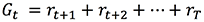
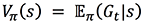
Before looking at methods to find optimal policies, you can formalize the objective of learning when the goal is to maximize the cumulative reward after a time step t by defining the concept of cumulative return Gt:

When there is a notion of a final step, each subsequence of actions is called an episode, and the MDP is said to have a finite horizon. If the agent-environment interaction goes on forever, the MDP is said to have an infinite horizon; in which case you can introduce a concept of discounting to define a mathematically unified notation for cumulative return:

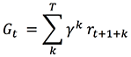
If γ = 1 and T is finite, this notation is the finite horizon formula for Gt, while if γ < 1, episodes naturally emerge even if T is infinite because terms with a large value of k become exponentially insignificant compared to terms with a smaller value of k. Thus the sum converges for infinite horizon MDP, and this notation applies for both finite and infinite horizon MDP.

Optimizing sequential decision-making with RL

There exists a large number of optimization methods that have been developed to solve the general RL problem. They are generally grouped into either policy-based methods or value-based methods, or combination thereof. We’ll focus mostly on the value-based methods as explained below.

Policy-based RL

In a policy-based RL, the policy is defined as a parametric function of some parameters θ: 𝜋θ = 𝜋(a|s,θ) and estimated directly by standard gradient methods. This is done by defining a performance measure, typically the expected value of Gt for a given policy, and applying gradient ascent to find θ that maximizes this performance measure. 𝜋θ can be any parameterized functional form of 𝜋 as long as 𝜋 is differentiable with respect to θ; thus a neural network can be used to estimate it, in which case the parameters θ are the weights of the neural network and the neural network predicts entire policies based on input states.

Direct policy search is relatively simple and also very limited because it attempts to estimate an entire policy directly from a set of previously experienced policies. Combining policy-based RL with value-based RL to refine the estimate of Gt almost always improves accuracy and convergence of RL, so this post focuses exclusively on value-based RL.

Value-based RL

An RL process is a Markov Decision Process (MDP), which is a mathematical formalization of sequential decision-making for which you can make precise statements. An MDP consists in a sequence (s0, a0, r1, s1, a1, r2, …, sn), or more generally (st, at, rt+1, st+1)n, and the dynamics of an MDP as illustrated in the previous diagram is fully characterized by a transition probability T(s,a,s’) = p(s’|s,a) that defines the probability for any state s to going to any other state s’, and a reward function r(s,a) = 𝔼(r|s,a) that defines the expected reward for any given state s.

Given the goal of RL is to learn the best policies to maximize Gt, this post first describes how to evaluate a policy in an MDP, and then how to go about finding an optimal policy.

To evaluate a policy, define a measure for any state s called a state value function V(s) that estimates how good it is to be in s for a particular way of acting, that is, for a particular policy 𝜋:

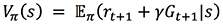
Recall from previous section that Gt is defined by the cumulative sum of rewards starting from current time step t up to final time step T. Replacing Gt by the right side of the equation defined in the previous section and moving rt+1 out of the summation, you get:

Replacing the expectation formula by a sum over all probabilities yields:

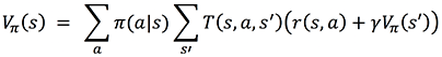
The latter is called the Bellman equation; it enables you to compute V𝜋(s) for an arbitrary 𝜋 based on T and r, computing the new value of V at time step t based on the previous value of V at time step t+1, recursively. You can estimate T and r by counting all the occurrences of observed transitions and rewards in a set of observed interactions between the agent and the environment. T and r define the model of the MDP.

Now you know how to evaluate a policy, you can extend the notion of state value function to the notion of state-action value function Q(s,a) to define an optimal policy:

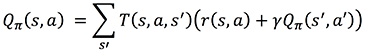
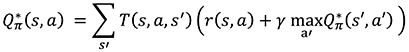
The latter is called the Bellman Optimality equation; it estimates the value of taking a particular action a in a particular state s assuming you’ll take the best actions thereafter. If you transform the Bellman Optimality equation into an assignment function you get an iterative algorithm that, assuming you know T and r, is guaranteed to converge to the optimal policy with random sampling of all possible actions in all states. Because you can apply this equation to states in any order, this iterative algorithm is referred to as asynchronous dynamic programming.

For systems in which you can easily compute or sample T and r, this approach is sufficient and is referred to as model-based RL because you know (previously computed) the transition dynamics (as characterized by T and r). But for most real-case problems, it is more convenient to produce stochastic estimates of the Q-values based on experience accumulated so far, so the RL agent learns in real time at every step and ultimately converges toward true estimates of the Q-values. To this end, combine asynchronous dynamic programming with the concept of moving average:

and replace Gt(s) by a sampled value as defined in the Bellman Optimality equation:

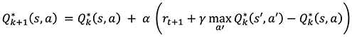
The latter is called temporal difference learning; it enables you to update the moving average Q*k+1(s,a) based on the difference between Q*k(s,a) and Q*k(s’,a’). This post shows a one-step temporal difference, as used in the most straightforward version of the Q-learning algorithm, but you could extend this equation to include more than one step (n-step temporal difference). Again, some theorems exist that prove Q-learning converges to the optimal policy 𝜋* assuming infinite random action selection.

RL action-selection strategy

You can alleviate the infinite random action selection condition by using a more efficient random action selection strategy such as ε-Greedy to increase sampling of states frequently encountered in good policies and decrease sampling of less valuable states. In ε-Greedy, the agent selects a random action with probability ε, and the rest of the time (that is, with probability 1 – ε), the agent selects the best action according to the latest Q-values, which is defined as .
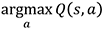
This strategy enables you to balance exploiting the latest Q-values with exploring new states and actions. Generally, ε is chosen to be large at the beginning to favor exploration of state-action space, and progressively reduced to a smaller value. For example, ε = 1% to exploit Q-values most of the time yet keep exploring and potentially discovering better policies.

Combining deep learning and reinforcement learning

In many cases, for example when playing chess or Go, the number of states, actions, and combinations thereof is so large that the memory and time needed to store the array of Q-values is enormous. There are more combinations of states and actions in the game Go than known stars in the universe. Instead of storing Q-values for all states and actions in an array which is impossible for Go and many other cases, deep RL attempts to generalize experience from a subset of states and actions to new states and actions. The following diagram is a comparison of Q-learning with look-up tables vs. function approximation.

Deep Q-learning uses a supervised learning approximation to Q(s,a) by using  
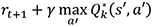
as the label, because the Q-learning assignment function is equivalent to a gradient update of the general form x  = x – ∝∇J (for any arbitrary x) where:

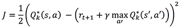
The latter is called the Square Bellman Loss; it allows you to estimate Q-values based on generalization from mapping states and actions to Q-values using a deep learning network, hence the name deep Q-learning.

Deep Q-learning is not guaranteed to converge anymore because the label used for supervised learning depends on current values of the network weights, which are themselves updated based on learning from the labels, hence a problem of broken ergodicity. But this approach is often good enough in practice and can generalize to the most complex RL problems (such as autonomous driving, robotics, or playing Go).                                                                      

In deep RL, the training set changes at every step, so you need to define a buffer to enable batch training, and schedule regular refreshes as experience accumulates for the agent to learn in real time. This is called experience replay and can be compared to the process of learning while dreaming in biological systems: experience replay allows you to keep optimizing policies over a subset of experiences (st, at, rt+1, st+1)n kept in memory.

This closes our theoretical journey on reinforcement learning and in particular the popular Deep Q-learning method, which implied several flavors of statistical learning, namely asynchronous dynamic programming, moving average, ε-Greedy and deep learning. Several RL variants exist in addition to the standard Deep Q-learning method, and Amazon SageMaker RL provides most of them out of the box, so after understanding one you will be able to test most of them using Amazon SageMaker RL.

Implementing a custom RL model in Amazon SageMaker

Application of reinforcement learning in financial services has received attention because better financial decisions can lead to high dollar return. In this post I implement a financial trading bot to demonstrate how to develop an agent that looks at the price of an asset over the past few days and decide whether to buy, sell, or do nothing, given the goal to maximize long-term profit.

I will benchmark this approach with another approach in which I combine reinforcement learning with recurrent deep neural networks for time series forecasting. In this second approach, the agent uses insights from multi-step horizon forecasts to make trading decisions and learn policies based on forecasted sequences of events rather than past sequences of events.

The data is a randomized version of a publicly available dataset on Yahoo Finance and represents price series for an arbitrary asset. For example, you can think of this data as the price of an EC2 Spot Instance or the market value of a publicly traded stock.

Setting up a built-in preset for deep Q-learning

In Amazon SageMaker RL, a preset file configures the RL training jobs and defines the hyperparameters for the RL algorithms. The following preset, for example, implements and parameterizes a deep Q-learning agent, as described in the previous section. It sets the number of steps to 2M. For more information about Amazon SageMaker RL hyperparameters and training jobs configuration, see Reinforcement Learning with Amazon SageMaker RL.

# Preset file in Amazon SageMaker RL

#################
# Graph Scheduling 
#################

schedule_params = ScheduleParameters()
schedule_params.improve_steps = TrainingSteps(2000000)
schedule_params.steps_between_evaluation_periods = EnvironmentSteps(10000)
schedule_params.evaluation_steps = EnvironmentEpisodes(5)
schedule_params.heatup_steps = EnvironmentSteps(0)

############
# DQN Agent 
############

agent_params = DQNAgentParameters()

# DQN params
agent_params.algorithm.num_steps_between_copying_online_weights_to_target = EnvironmentSteps(100)
agent_params.algorithm.discount = 0.99
agent_params.algorithm.num_consecutive_playing_steps = EnvironmentSteps(1)

# NN configuration
agent_params.network_wrappers['main'].learning_rate = 0.00025
agent_params.network_wrappers['main'].replace_mse_with_huber_loss = False

# ER size
agent_params.memory.max_size = (MemoryGranularity.Transitions, 40000)

# E-Greedy schedule
agent_params.exploration.epsilon_schedule = LinearSchedule(1.0, 0.01, 200000)

#############
# Environment 
#############

env_params = GymVectorEnvironment(level='trading_env:TradingEnv')

##################
# Manage resources 
##################

preset_validation_params = PresetValidationParameters()
preset_validation_params.test = True

graph_manager = BasicRLGraphManager(agent_params=agent_params, env_params=env_params,
                                    schedule_params=schedule_params, vis_params=VisualizationParameters(),
                                    preset_validation_params=preset_validation_params)

Setting up a custom OpenAI Gym RL environment

In Amazon SageMaker RL, most of the components of an RL Markov Decision Process as described in the previous section are defined in an environment file. You can connect open-source and custom environments developed using OpenAI Gym, which is a popular set of interfaces to help define RL environments and is fully integrated into Amazon SageMaker. The RL environment can be the real world in which the RL agent interacts or a simulation of the real world. You can simulate the real world by a daily series of past prices. To formulate the bidding problem into an RL problem, you need to define each of the following components of the MDP:

  • Environment – Custom environment that generates a simulated price with daily and weekly variations and occasional spikes
  • State – Daily price of the asset over the past 10 days
  • Action – Sell or buy the asset, or do nothing, on a daily basis
  • Goal – Maximize accumulated profit
  • Reward – Positive reward equivalent to daily profit, if any, and a penalty equivalent to the price paid for any asset purchased

A custom file called TradingEnv.py specifies all these components. It is located in the src/ folder and called by the preset file defined earlier. In particular, the size of the state space (n = 10 days) and the action space (m = 3) are defined using OpenAI Gym through the following lines of code:

# Custom environment file in Open AI Gym and Amazon SageMaker RL

class TradingEnv(gym.Env):

    def __init__(self,casset = 'asset_prices', span = 10 ):
        
        self.asset = asset
        self.span = span
                
        # Read input data 
        datafile = DATA_DIR + asset + '.csv'
        self.data = pd.read_csv(datafile) 
        self.observations = self.getObservations(datafile)
        
        # Number of time steps in data file
        self.steps = len(self.observations) - 1
        
        # Output filename
        self.csv_file = CSV_DIR
        
        # Action 
        self.action_space = gym.spaces.Discrete(3)

        # Observation space is defined from the data min and max
        self.observation_space = gym.spaces.Box(low = -np.inf, high = np.inf, shape = (self.span,), dtype = np.float32)

        (…)

The goal is translated into a quantitative reward function, as explained in the previous section, and this reward function is also formulated in the environment file. See the following code:

# Definition of reward function
def step(self, action):
        
    # BUY:
    if action == 1: 		
        self.inventory.append(self.observations[self.t])
        margin = 0  
        reward = 0
    # SELL:
    elif action == 2 and len(self.inventory) > 0: 
        bought_price = self.inventory.pop(0)
        margin = self.observations[self.t] - bought_price
        reward = max(margin, 0)            
    # SIT:
    else: 
        margin = 0
        reward = 0

    self.total_profit += margin
            
    # Increment time
    self.t += 1
        
    # Store state for next day
    obs = self.getState(self.observations, self.t, self.span + 1, self.mode)
            
    # Stop episode when reaches last time step in file
    if self.t >= self.steps:
        done = True 
    else:
        done = False

   (…)             
   
    return obs, reward, done, info 

Launching an Amazon SageMaker RL estimator

After defining a preset and RL environment in Amazon SageMaker RL, you can train the agent by creating an estimator following a similar approach to when using any other ML estimators in Amazon SageMaker. The following code shows how to define an estimator that calls the preset (which itself calls the custom environment):

# Definition of the RL estimator in Amazon SageMaker RL

estimator = RLEstimator(source_dir='src',
                        entry_point=entryfile,
                        dependencies=["common/sagemaker_rl"],
                        toolkit=RLToolkit.COACH,
                        toolkit_version='0.11.0',
                        framework=RLFramework.MXNET,
                        role=role,
                        train_instance_count=1,
                        train_instance_type='ml.c5.9xlarge',
                        output_path=s3_output_path,
                        base_job_name=job_name_prefix,
                        hyperparameters = {"RLCOACH_PRESET" : "preset-trading"})

You would generally use a config.py file in Amazon SageMaker RL to define global variables, such as the location of a custom data file in the Amazon SageMaker container. See the following code:

# Configuration file (config.py) used to define global variables in Amazon SageMaker RL

import os
CUR_DIR = os.path.dirname(__file__)
DATA_DIR = CUR_DIR + '/datasets/' 
CSV_DIR = '/opt/ml/output/data/simulates.csv'

Training and evaluating the RL agent’s performance

This section demonstrates how to train the RL bidding agent in a simulation environment constructed using seven years of daily historical transactions. You can evaluate learning during the training phase and evaluate the performance of the trained RL agent at generalizing on a test simulation, here constructed using three additional years of daily transactions. You can assess  the agent’s ability to learn and generalize by visualizing the accumulated reward and accumulated profit per episode during the training and test phases.

Evaluating learning during training of the RL agent

In reinforcement learning, you can train an agent by simulating interactions (st, at, rt+1, st+1) with the environment and computing the cumulative return Gt, as described previously. After an initial exploration phase, as the value of ε in ε-Greedy progressively decreases to favor exploitation of learned policies, the total accumulated reward in a given episode accounts for how good the policy followed was. Thus, the total accumulated reward compared between episodes enables you to evaluate the relative quality of the policies learned. The following graphs show the reward and profit accumulated by the RL agent during training simulations. The x-axis is the episode index and the y-axis is the reward or profit accumulated per episode by the RL agent.

The graph on accumulated reward shows a trend with essentially three phases: relatively large fluctuations during the first 300 episodes (exploration phase), steady growth between 300 and 500 episodes, and a plateau (500–800 episodes) in which the total accumulated reward has reached convergence and revolves around a relatively stable value of $1,800.

Consistently, the accumulated profit is approximately zero during the first 300 episodes and revolves around a relatively stable value of $800 after episode 500.

Together, these results indicate that the RL agent has learned to trade the asset profitably, and has converged toward a stable behavior with reproducible policies to generate profit over the training dataset.

Evaluating generalization on a test set of the RL agent

To evaluate the agent’s ability to generalize to new interactions with the environment, you can constrain the agent to exploit the learned policies by setting the value of ε to zero and simulate new interactions (st, at, rt+1, st+1) with the environment.

The following graph shows the profit generated by the RL agent during test simulations. The x-axis is the episode index and the y-axis is profit accumulated per episode by the RL agent.

The graph shows that after three years of new daily prices for the same asset, the trained agent tends to generate profits with a mean of $2,200 and standard deviation of $600 across 65 test episodes. In contrast to the training simulations, you can observe a steady mean across all 65 test episodes simulated, indicating a strong convergence of the policies learned.

The graph confirms that the RL agent has converged and learned reproducible policies to trade the asset profitably and can generalize to new prices and trends.

Benchmarking a deep recurrent RL agent

Finally, I benchmarked the results from the previous deep RL approach with a deep recurrent RL approach. Instead of defining a state as a window of the past 10 days, an RNN for time series forecasting encodes the state as a 10-day horizon forecast, so the agent benefits from an advisor on future expected prices when learning optimal trading policies for maximizing long-term return.

Implementing a forecast-based RL state space

The following code implements a simple RNN for time series forecasting, following the post Forecasting financial time series with dynamic deep learning on AWS:

# Custom function to define a RNN for time series forecasting

def trainRNN(self, data, lag, horiz, nfeatures):

        # Set hyperparameters
        nunits = 64                         # Number of GRUs in recurrent layer
        nepochs = 1000                 # Number of epochs
        d = 0.2                                 # Percent of neurons to drop at each epoch
        optimizer = 'adam'            # Optimization algorithm
        activ = 'elu'                         # Activation function of neurons
        activr = 'hard_sigmoid'.   # Activation function of recurrent layer
        activd = 'linear'                  # Dense layer's activation function
        lossmetric = 'mean_absolute_error'  # Loss function for gradient descent
        verbose = False                  # Print results on standard output channel

        # Prepare data
        df = data
        df["Adjclose"] = df.Close 
        df.drop(['Date','Close','Adj Close'], 1, inplace=True)
        df = df.diff() 

        data = df.as_matrix()
        lags = []
        horizons = []
        nsample = len(data) - lag - horiz  
        for i in range(nsample):
                lags.append(data[i: i + lag , -nfeatures:])
                horizons.append(data[i + lag : i + lag + horiz, -1])
        lags = np.array(lags)
        horizons = np.array(horizons)
        lags = np.reshape(lags, (lags.shape[0], lags.shape[1], nfeatures))

        # Design RNN architecture
        rnn_in = Input(shape = (lag, nfeatures), dtype = 'float32', name = 'rnn_in')
        rnn_gru = GRU(units = nunits, return_sequences = False, activation = activ, recurrent_activation = activr, dropout = d)(rnn_in)
        rnn_out = Dense(horiz, activation = activd, name = 'rnn_out')(rnn_gru)
        model = Model(inputs = [rnn_in], outputs = [rnn_out])
        model.compile(optimizer = optimizer, loss = lossmetric)

        # Train model
        fcst = model.fit({'rnn_in': lags},{'rnn_out': horizons}, epochs=nepochs,verbose=verbose)

And the following function redirects the agent to an observation based on lag or forecasted horizon (the two types of RL approaches discussed in this post), depending on the value of a custom global variable called mode:

# Custom function to define a state at time t

def getState(self, observations, t, lag, mode):

# Mode "past": State at time t defined as n-day lag in the past
if mode == 'past':
     d = t - lag + 1
     block = observations[d:t + 1] if d >= 0 else -d * [observations[0]] + observations[0:t + 1] # pad with t0
     res = []
     for i in range(lag - 1):
             res.append(self.sigmoid(block[i + 1] - block[i]))
     return np.array([res])

# Mode "future": State at time t defined as the predicted n-day horizon in the future using RNN
elif mode == 'future':
     rnn = load_model(self.rnn_model)
     d = t - lag + 1
     block = observations[d:t + 1] if d >= 0 else -d * [observations[0]] + observations[0:t + 1] # pad with t0
     horiz = rnn.predict(block)
     res = []
     for i in range(lag - 1): 
             res.append(self.sigmoid(horiz[i + 1] - horiz[i]))
  

Evaluating learning during training of the RNN-based RL agent

As in the previous section for the RL agent in which a state is defined as the lag of the past 10 observations (referred to as lag-based RL), you can evaluate the relative quality of the policies learned by the RNN-based agent by comparing the total accumulated reward between episodes.

The following graphs show the reward and profit accumulated by the RNN-based RL agent during training simulations. The x-axis is the episode index and the y-axis is the reward or profit accumulated per episode by the RL agent.

The graph on accumulated reward shows a steady growth after episode 300, and most episodes after episode 500 result in an accumulated reward of approximately $1,000. But several episodes result in a much higher reward of up to $8,000.

The accumulated dollar profit is approximately zero during the first 300 episodes, revolves around a positive value after episode 500, with again several episodes where the generated profit reaches up to $7,500.

Together, these results indicate that the RL agent has learned to trade the asset profitably, and has converged toward a behavior with policies that generate profit either around $500–800, or some much higher values up to $7,500, over the training dataset.

Evaluating generalization on a test set of the RNN-based RL agent

The following graph shows the profit in dollars generated by the RNN-based RL agent during test simulations. The x-axis is the episode index and the y-axis is the profit accumulated per episode by the RL agent.

The graph shows that the RNN-based RL agent can generalize to new prices and trends. Consistent with the observations made during training, it shows that after three years of new daily prices for the same asset, the trained agent tends to generate profits around $2,000, or some much higher profit up to $7,500. This dual behavior is characterized by an overall mean of $4,900 and standard deviation of $3,000 across the 65 test episodes.

The minimum profit across all 65 test episodes simulated is $1,300, while it was $1,500 for the lag-based RL approach. The maximum profit is $7,500, with frequent accumulated profit over $5,000, while it was only $2,800 for the lag-based RL approach. Thus, the RNN-based RL approach results in higher volatility compared to the lag-based RL approach, but exclusively toward higher profits which is a better outcome given the goal of the RL problem is to generate profit.

The results between the lag-based RL agent and the RNN-based RL agent confirm that the RNN-based RL agent is more beneficial. It has learned reproducible policies to trade the asset that are either similar to, or significantly outperform, the policies learned by the lag-based agent for generating profit.

Conclusion

In this post, I introduced the motivations and underlying theoretical concepts behind deep reinforcement learning, an ML solution framework that enables you to learn and apply optimal policies given a long-term objective. You have seen how to use Amazon SageMaker RL to develop and train a custom deep RL agent to make smart decisions in real time in an arbitrary bidding environment.

You have also seen how to evaluate the performance of the deep RL agent during training and test simulations, and how to benchmark its performance against a more advanced, deep recurrent RL based on RNN for time series forecasting.

This post is for educational purposes only. Past trading performance does not guarantee future performance. The loss in trading can be substantial; investors should use all trading strategies at their own risk.

For more information about popular RL algorithms, sample codes, and documentation, you can visit Reinforcement Learning with Amazon SageMaker RL.


About the Author

Jeremy David Curuksu is a data scientist at AWS and the global lead for financial services at Amazon Machine Learning Solutions Lab. He holds a MSc and a PhD in applied mathematics, and was a research scientist at EPFL (Switzerland) and MIT (US). He is the author of multiple scientific peer-reviewed articles and the book Data Driven, which introduces management consulting in the new age of data science.


Building an NLP-powered search index with Amazon Textract and Amazon Comprehend

Organizations in all industries have a large number of physical documents. It can be difficult to extract text from a scanned document when it contains formats such as tables, forms, paragraphs, and check boxes. Organizations have been addressing these problems with Optical Character Recognition (OCR) technology, but it requires templates for form extraction and custom workflows.

Extracting and analyzing text from images or PDFs is a classic machine learning (ML) and natural language processing (NLP) problem. When extracting the content from a document, you want to maintain the overall context and store the information in a readable and searchable format. Creating a sophisticated algorithm requires a large amount of training data and compute resources. Building and training a perfect machine learning model could be expensive and time-consuming.

This blog post walks you through creating an NLP-powered search index with Amazon Textract and Amazon Comprehend as an automated content-processing pipeline for storing and analyzing scanned image documents. For pdf document processing, please refer AWS Sample github repository to use Textractor.

This solution uses serverless technologies and managed services to be scalable and cost-effective. The services used in this solution include:

Architecture

  1. Users upload OCR image for analysis to Amazon S3.
  2. Amazon S3 upload triggers AWS Lambda.
  3. AWS Lambda invokes Amazon Textract to extract text from image.
  4. AWS Lambda sends the extracted text from image to Amazon Comprehend for entity and key phrase extraction.
  5. This data is indexed and loaded into Amazon Elasticsearch.
  6. Kibana gets indexed data.
  7. Users log into Amazon Cognito.
  8. Amazon Cognito authenticates to Kibana to search documents.

Deploying the architecture with AWS CloudFormation

The first step is to use an AWS CloudFormation template to provision the necessary IAM role and AWS Lambda function to interact with the Amazon S3, AWS Lambda, Amazon Textract, and Amazon Comprehend APIs.

  1. Launch the AWS CloudFormation template in the US-East-1 (Northern Virginia) Region:
  2. You will see the below information on the Create stack screen:
    Stack name: document-search
    CognitoAdminEmail: abc@amazon.com
    DOMAINNAME: documentsearchapp.Edit the CognitoAdminEmail with your email address. You will receive your temporary Kibana credentials in an email.
  3. Scroll down to Capabilities and check both the boxes to provide acknowledgement that AWS CloudFormation will create IAM resources. For more information, see AWS IAM resources.
  4. Scroll down to Transforms and choose Create Change Set.The AWS CloudFormation template uses AWS SAM, which simplifies how to define functions and APIs for serverless applications, as well as features for these services like environment variables. When deploying AWS SAM templates in an AWS CloudFormation template, you need to perform a transform step to convert the AWS SAM template.
  5. Wait a few seconds for the change set to finish computing changes. Your screen should look as follows with Action, Logical Id, Physical Id, Resource Type, and Replacement. Finally, click on the Execute button, which will let AWS CloudFormation launch resources in the background.
  6. The following screenshot of the Stack Detail page shows the Status of the CloudFormation stack as CREATE_IN_PROGRESS. Wait up to 20 minutes for the Status to change to CREATE_COMPLETE. In Outputs, copy the value of S3KeyPhraseBucket and KibanaLoginURL.

Uploading documents to the S3 bucket

To upload your documents to your newly created S3 bucket in the above step, complete the following:

  1. Click on the Amazon S3 Bucket URL you copied from the CloudFormation Output.
  2. Download the example dataset demo-data.zip from the GitHub repo. This dataset contains a variety of images that include forms, a scanned page with paragraphs, and a two-column document.
  3. Unzip the data.
  4. Upload the files in the demo-data folder to the Amazon S3 bucket starting with document-search-blog-s3-<Random string>.

For more information, see How Do I Upload Files and Folders to an S3 Bucket?

After the upload completes, you can see four image files: Employment_application.JPG, expense.png, simple-document-image.jpg, and two-column-image.jpg in the S3 bucket.

Uploading the data to S3 triggers a Lambda S3 event notification to invoke a Lambda function. You can find event triggers configured in your Amazon S3 bucket properties under Advanced settings-> Events. You will see a Lambda function starting with document-search-blog-ComprehendKeyPhraseAnalysis-<Random string>. This Lambda function performs the following:

  • Extracts text from images using Amazon Textract.
  • Performs key phrase extraction using Amazon Comprehend.
  • Searches text using Amazon ES.

The following code example extracts text from images using Amazon Textract:

textract = boto3.client(

service_name='textract',

region_name=region)

#Main lambda handler
def handler(event, context):
    # Get the object from the lambda event and show its content type
       bucket = event['Records'][0]['s3']['bucket']['name']
       key = unquote_plus(event['Records'][0]['s3']['object']['key'])
       s3.Bucket(bucket).download_file(Key=key,Filename='/tmp/{}')
# Read document content and extract text using Textract
with open('/tmp/{}', 'rb') as document:
    imageBytes = bytearray(document.read())
response=textract.analyze_document(Document={'Bytes':imageBytes},FeatureTypes=["TABLES", "FORMS"])

The following code example extracts key phrases using Amazon Comprehend:

#Initializing comprehend
comprehend = boto3.client(service_name='comprehend', region_name=region)
#Detect Keyphrases and Entities
keyphrase_response = comprehend.detect_key_phrases(Text=text, LanguageCode='en')
detect_entity= comprehend.detect_entities(Text=text, LanguageCode='en')

You can index the response received from Amazon Textract and Amazon Comprehend and load it into Amazon ES to create an NLP-powered search index. Refer to the below code:

 #Connection to Elasticsearch
         
        es=connectES()
#Saving Index to Elastocsearch endpoint in primary lambda handler    

        es.index(index="document", doc_type="_doc", body=searchdata)

For more information, see the GitHub repo.

Visualizing and searching documents with Kibana

To visualize and search documents using Kibana, perform the following steps.

  1. Find the email in your inbox with the subject line “Your temporary password.” Check your junk folder if you don’t see an email in your inbox.
  2. Go to the Kibana login URL copied from the AWS CloudFormation output.
  3. Login using your email address as the Username and the temporary password from the confirmation email as the Password.  Click on Sign In.

    Note: If you didn’t receive the email or missed it while deploying AWS CloudFormation, choose Sign up.
  4. On the next page, enter a new password.
  5. On the Kibana landing page, from the menu, choose Discover.
  6. On the Management/Kibana page, you will see Step 1 of 2: Define index pattern, for Index pattern, enter document*. The message “Success! Your index pattern matches 1 index.” appears. Choose Next step. Click Create Index Pattern.
    After a few seconds, you can see the document index page.
  7. Choose Discover from the menu again. In the below screenshot you can see the document attributes.
    s3link:s3 location of uploaded documents in S3, 
    KeyPhrases: Key phrases from the documents uploaded in S3, 
    Entity: it can be DATE, PERSON, ORGANIZATION etc, 
    text: raw text from documents, 
    table:tables extracted from documents, and forms:form extracted from documents 

  8. To view specific fields for each entry, hover over the field in the left sidebar and click Add.

This moves the fields to the Selected Fields menu. Your Kibana dashboard formulates data in an easy-to-read format. The following screenshot shows the view after adding Entity.DATE, Entity.Location, Entity.PERSON, S3link and text in the Selected Fields menu:

To look at your original document, choose s3link.

Note: You can also add forms and table to view and search tables and forms.

Conclusion

This post demonstrated how to extract and process data from an image document and visualize it to create actionable insights.

Processing scanned image documents helps you uncover large amounts of data, which can provide new business prospects. With managed ML services like Amazon Textract and Amazon Comprehend, you can gain insights into your previously undiscovered data. For example, you could build a custom application to get a text from a scanned legal document, purchase receipts, and purchase orders.

Data at scale is relevant in every industry. Whether you process data from images or PDFs, AWS can simplify your data ingestion and analysis while keeping your overall IT costs manageable.

If this blog post helps you or inspires you to solve a problem, we would love to hear about it! The code for this solution is available on the GitHub repo for you to use and extend. Contributions are always welcome!


About the authors

Saurabh Shrivastava is a partner solutions architect and big data specialist working with global systems integrators. He works with AWS partners and customers to provide them with architectural guidance for building scalable architecture in hybrid and AWS environments. He enjoys spending time with his family, outdoor activity, and traveling to new destinations to discover new cultures.


Mona is an AI/ML specialist solutions architect working with the AWS Public Sector Team. She works with AWS customers to help them with the adoption of Machine Learning on a large scale. She enjoys painting and cooking in her free time.


How AWS is putting machine learning in the hands of every developer and BI analyst

Today AWS announced new ways for you to easily add machine learning (ML) predictions to applications and business intelligence (BI) dashboards using relational data in your Amazon Aurora database and unstructured data in Amazon S3, by simply adding a few statements to your SQL (structured query language) queries and making a few clicks in Amazon QuickSight. Aurora, Amazon Athena, and Amazon QuickSight make direct calls to AWS ML services like Amazon SageMaker and Amazon Comprehend so you don’t need to call them from your application. This makes it more straightforward to add ML predictions to your applications without the need to build custom integrations, move data around, learn separate tools, write complex lines of code, or even have ML experience.

These new changes help make ML more usable and accessible to database developers and business analysts by making sophisticated ML predictions more readily available through SQL queries and dashboards. Formerly, you could spend days writing custom application-level code that must scale and be managed and supported in production. Now anyone who can write SQL can make and use predictions in their applications without any custom “glue code.”

Making sense of a world awash in data

AWS firmly believes that in the not-too-distant future, virtually every application will be infused with ML and artificial intelligence (AI). Tens of thousands of customers benefit from ML through Amazon SageMaker, a fully managed service that allows data scientists and developers the ability to quickly and easily build, train, and deploy ML models at scale.

While there are a variety of ways to build models, and add intelligence to applications through easy-to-use APIs like Amazon Comprehend for example, it can still be challenging to incorporate these models into your databases, analytics, and business intelligence reports. Consider a relatively simple customer service example. Amazon Comprehend can quickly evaluate the sentiment of a piece of text (is it positive or negative?). Suppose that I leave feedback on a store’s customer service page: “Your product stinks and I’ll never buy from you again!” It would be trivial for the store to run sentiment analysis on user feedback and contact me immediately to make things right. The data is available in their database and ML services are widely available.

The problem, however, lies in the difficulty of building prediction pipelines to move data between models and applications.

Developers have historically had to perform a large amount of complicated manual work to take these predictions and make them part of a broader application, process, or analytics dashboard. This can include undifferentiated, tedious application-level code development to copy data between different data stores and locations and transform data between formats, before submitting data to the ML models and transforming the results to use inside your application. Such work tends to be cumbersome and a poor way to use the valuable time of your developers. Moreover, moving data in and out of data stores complicates security and governance.

Putting machine learning in the hands of every developer

At AWS, our mission is clear: we aim to put machine learning in the hands of every developer. We do this by making it easier for you to become productive with sophisticated ML services. Customers of all sizes, including NFL, Intuit, AstraZeneca, and Celgene, rely on AWS ML services such as Amazon SageMaker and Amazon Comprehend. Celgene, for example, uses AWS ML services for toxicology prediction to virtually analyze the biological impacts of potential drugs without putting patients at risk. A model that previously took two months to train can now be trained in four hours.

While AWS offers the broadest and deepest set of AI and ML services, and though we introduced more than 200 machine learning features and capabilities in 2018 alone, we’ve felt that more is needed. Among these other innovations, one of the best things we can do is to enable your existing talent to become productive with ML.

And, specifically, developer talent and business analyst talent.

Though we offer services that improve the productivity of data scientists, we want to give the much broader population of application developers access to fully cloud-native, sophisticated ML services. Tens of thousands of customers use Aurora and are adept at programming with SQL. We believe it is crucial to enable you to run ML learning predictions on this data so you can access innovative data science without slowing down transaction processing. As before, you can train ML models against your business data using Amazon SageMaker, with the added ability to run predictions against those same models with one line of SQL using Aurora or Athena. This makes the results of ML models more accessible for a broad population of application developers.

Lead scoring is a good example of how this works. For example, if you build a CRM system on top of Aurora, you’ll store all of your customer relationship data, marketing outreach, leads, etc. in the database. As leads come from the website they’re moved to Aurora, and your sales team follows up on the leads convert them to customers.

But what if you wanted to help make that process more effective for your sales team? Lead scoring is a predictive model which helps qualify and rank incoming leads so that the sales team can prioritize which leads are most likely to convert to a customer sale, making them more productive. You can take a lead scoring model built by your data science team, or one that you have purchased on the AWS ML Marketplace, deploy it to Amazon SageMaker, and then order all your sales queues by priority based on the prediction from the model. Unlike in the past, you needn’t write any glue code.

Or you might want to use these services together to deliver on a next best offer use case. For example, your customer might phone into your call center complaining about an issue. The customer service representative successfully addresses the issue and proceeds to offer new products or services. How? Well, the representative can pull up a product recommendation on the Amazon QuickSight dashboard that shows multiple views and suggestions.

The first view shows product recommendations based on an Aurora query. The query pulls the customer profile, shopping history, and product catalog, and calls a model in Amazon SageMaker to make product recommendations. The second view is an Athena query that pulls customer browsing history or clickstream data from an S3 data lake, and calls an Amazon SageMaker model to make product recommendations. The third view is an Amazon QuickSight query that takes results from first and second view, calls an ensemble model in Amazon SageMaker, and makes the recommendations. You now have several offers to make based on different views of the customer, and all within one dashboard.

On the BI analyst side, we regularly hear from customers that it’s frustrating to have to build and manage prediction pipelines before getting predictions from a model. Developers currently spend days writing application-level code to move data back and forth between models and applications. You may now choose to deprecate your prediction pipelines and instead use Amazon QuickSight to visualize and report on all your ML predictions.

For application developers and business analysts, these changes make it more straightforward to add ML predictions to your applications without the need to build custom integrations, move data around, learn separate tools, write complex lines of code, or even have ML experience. Instead of days of developer labor, you can now add a few statements to your SQL queries and make a few clicks in Amazon QuickSight.

In these ways, we’re enabling a broader population of developers and data analysts to tap into the power of ML, with no Ph.D. required.


About the Author

Matt Asay (pronounced “Ay-see”) is a principal at AWS, and has spent nearly two decades working for a variety of open source and big data companies. You can follow him on Twitter (@mjasay).


Amazon Transcribe now supports speech-to-text in 31 languages

We recently announced that Amazon Transcribe now supports transcription for audio and video for 7 additional languages including Gulf Arabic, Swiss German, Hebrew, Japanese, Malay, Telugu, and Turkish languages.  Using Amazon Transcribe, customers can now take advantage of 31 supported languages for transcription use cases such as improving customer service, captioning and subtitling, meeting accessibility requirements, and cataloging audio archives.

Using Amazon Transcribe

Amazon Transcribe is an easy-to-use automatic speech recognition (ASR) service that makes it easy to analyze audio files and convert those into text that includes enrichment such as speaker identification, timestamp generation, punctuation, and formatting. With the recent announcement, customers can now transcribe audio from even more languages.

Using the AWS Management Console, let’s check out one of the latest languages in action. Amazon Transcribe allows users to transcribe streaming audio or perform asynchronous transcription.  For this, we will create a job for asynchronous transcription using an audio file stored in Amazon S3 as input.

Upon completion of the job, the audio-to-text transcription is provided in the response.   For those of us that don’t know Turkish, you can then run your transcribed text through the Amazon Translate service to translate the transcribed text into your preferred language.

In the example above, we are using the console to create the transcription job; however, customers can also programmatically submit transcription jobs using the Amazon Transcribe APIs.   The APIs are available in the AWS SDKs.  The example below demonstrates invoking the Amazon Transcribe APIs through the AWS CLI:

Start Transcription Job

$ aws transcribe start-transcription-job --transcription-job-name Transcribe-Turkish-Audio-CLI --language-code tr-TR --media MediaFileUri=s3://whats-new-transcribe/Turkish-Audio.mp3 --media-format mp3 --region us-east-1
{
    "TranscriptionJob": {
        "TranscriptionJobName": "Transcribe-Turkish-Audio-CLI", 
        "LanguageCode": "tr-TR", 
        "TranscriptionJobStatus": "IN_PROGRESS", 
        "Media": {
            "MediaFileUri": "s3://whats-new-transcribe/Turkish-Audio.mp3"
        }, 
        "CreationTime": 1574392674.948, 
        "MediaFormat": "mp3"
    }
}

Get Information about Transcription Job

$ aws transcribe get-transcription-job --transcription-job-name Transcribe-Turkish-Audio-CLI --region us-east-1
{
    "TranscriptionJob": {
        "TranscriptionJobName": "Transcribe-Turkish-Audio-CLI", 
        "LanguageCode": "tr-TR", 
        "MediaSampleRateHertz": 22050, 
        "TranscriptionJobStatus": "COMPLETED", 
        "Settings": {
            "ChannelIdentification": false
        }, 
        "Media": {
            "MediaFileUri": "s3://whats-new-transcribe/Turkish-Audio.mp3"
        }, 
        "CreationTime": 1574392674.948, 
        "CompletionTime": 1574392772.813, 
        "MediaFormat": "mp3", 
        "Transcript": {
            "TranscriptFileUri": "https://s3.amazonaws.com/aws-transcribe-us-east-1-prod/"
        }
    }
}

Because we did not explicitly specify a bucket to direct transcription output to, the transcription result is provided via a presigned URL that provides secure access to that transcription.  Using the TranscriptFileUri returned on output, we can view/parse that JSON object returned for the transcript text returned.

The transcribed text can then be used for a variety of use cases such as input into Amazon Comprehend for identification of key phrases and key entities such as names, organization names, or as input into Amazon Translate as shown above for translation into one or more languages.

Amazon Transcribe and Amazon Translate for multilingual subtitles

The combined capability of using Amazon Transcribe and Amazon Translate allows customers to quickly transcribe audio as well as convert it into multiple target languages for meeting globalization requirements as well as use cases such as extended global reach on videos or adding subtitles to training videos for your organization.  These capabilities can be extended into multilingual subtitles for videos and podcasts. Providing these capabilities allows users to extend global reach by including more language options for broader audiences.

AWS Architecture provides a quick start solution and deployment guide customers can leverage for Live Streaming with Automated Multi-Language Subtitling.   This real-time subtitling solution for live streaming video generates multi-language subtitles for live streaming videos using Amazon Transcribe for audio-to-text and Amazon Translate for language translation.

Available Now!

These new languages are available today in all Regions where Amazon Transcribe is available. The free tier offers 60 minutes per month for the first 12 months, starting from your first transcription request.

We’re looking forward to your feedback! Please post it to the AWS Forum for Amazon Transcribe, or send it to your usual AWS Support contacts.


About the author

Shelbee Eigenbrode is a solutions architect at Amazon Web Services (AWS). Her current areas of depth include DevOps combined with machine learning and artificial intelligence. She’s been in technology for 22 years, spanning multiple roles and technologies. In her spare time she enjoys reading, spending time with her family, friends and her fur family (aka. dogs).