Blog

Learn About Our Meetup

5000+ Members

MEETUPS

LEARN, CONNECT, SHARE

Join our meetup, learn, connect, share, and get to know your Toronto AI community. 

JOB POSTINGS

INDEED POSTINGS

Browse through the latest deep learning, ai, machine learning postings from Indeed for the GTA.

CONTACT

CONNECT WITH US

Are you looking to sponsor space, be a speaker, or volunteer, feel free to give us a shout.

Category: Amazon

Engage listeners with Amazon Polly’s Conversational speaking style voices

All voices are unique, yet speakers tend to adjust their delivery, or speaking style, according to their context and audience. Before Amazon Polly used Neural Text-to-Speech technology (NTTS) to build voices, TTS (Standard Text-to-Speech) voices couldn’t change their speech patterns to match any particular speaking style. When Amazon Polly introduced NTTS, Newscaster voices were launched as the first speaking style.

Matthew and Joanna, two of the US English voices in the Amazon Polly portfolio, are now also available in a Conversational speaking style, which simulates the speech patterns of a friendly conversation. Similar to how people learn to talk as a children, TTS voices acquire intonation patterns from natural speech data, then try to reproduce synthesized utterances in similar manners. Amazon Polly’s NTTS technology, a neural network-based machine learning model, makes this learning possible. It is capable of picking up nuances in various speaking styles and applying them when synthesizing text into speech.

Pillo Health is a startup that uses Amazon Polly to voice their in-home devices. Paige Baeder, Pillo Health’s product manager, says, “Pillo Health serves individuals who manage chronic conditions in the comfort of their home. Maintaining our community’s trust starts with each daily interaction. The Conversational version of Amazon Polly’s Joanna voice provides clarity and expression that inspires trust and is easy to understand, allowing us to connect with our users through a voice that brings Pillo (our in-home companion device) persona to life. Making the decision to switch to Joanna in Amazon Polly was easy—it was the top pick amongst all of our voice testers.”

Unlike traditional synthesis approaches that rely heavily on constructed rules, NTTS builds its own model based on given training data. Dynamic intonation and expressiveness used to be obstacles because linguistic rules could not cover them, but now they are the key to voices sounding natural in NTTS. The system needs to recognize the diversity in speech, in order to mimic it when generating speech. In the studio, Amazon Polly’s voice talents record in an engaging tone, as they would when they engage in normal day-to-day conversation. A few characteristics of natural speech include reduced syllables, pitch change, pausing, and contractions. The recording script for training data is carefully designed based on common utterances, which helps deliver natural speech data.

The Conversational speaking style feature generally makes neural voices sound more friendly and expressive. For example, listen to the following audio sample from Matthew in the Conversational speaking style, as compared to the neutral neural style (speaking-style free):

Neutral sample (Matthew)

Listen now

Voiced by Amazon Polly

Conversational sample (Matthew)

Listen now

Voiced by Amazon Polly

In the Conversational speech sample, the word “sorry” is emphasized with a slight pause and a stress, which sounds more empathetic in this given situation. The question also sounds more friendly in the Conversational version, providing a better user experience.

Here’s Joanna introducing the Conversational style:

Neutral sample (Joanna)

Listen now

Voiced by Amazon Polly

Conversational sample (Joanna)

Listen now

Voiced by Amazon Polly

To synthesize the Conversational style, make sure to enclose the input with the following SSML tag and set the text type to ssml in the command line:

<speak>
<amazon:domain name="conversational">
We are excited to share that Matthew and Joanna, the US English voices available in Polly, sound more natural thanks to the conversational style.
</amazon:domain>
</speak>
$ aws polly start-speech-synthesis-task
       --voice-id Joanna --engine neural
       --text file://s3.ssml --text-type ssml
       --output-s3-bucket-name "polly-conversational-synth" --output-format mp3
       --query "SynthesisTask.TaskId"
       "14e73ba4-ec52-4811-b597-9b07a368c213"
$ wget https://polly-conversational-synth.s3.amazonaws.com/14e73ba4-ec52-4811-b597-9b07a368c213.mp3 -O joanna-conversational.mp3

You can trigger the Conversational speaking style with US English voices Matthew and Joanna within the Amazon Polly console, AWS CLI, or SDK. The feature is currently available in US East (N. Virginia), US West (Oregon), and EU (Ireland) Regions. For more information, see What Is Amazon Polly?


About the author

Chiao-ting Fang is a TTS language engineer for Amazon text-to-speech. She enjoys applying her linguistic knowledge at work to build better, more natural-sounding voices. She loves languages, traveling, and star-gazing.


Announcing Amazon Rekognition Custom Labels

Today, Amazon Web Services (AWS) announced Amazon Rekognition Custom Labels, a new feature of Amazon Rekognition that enables customers to build their own specialized machine learning (ML) based image analysis capabilities to detect unique objects and scenes integral to their specific use case. For example, customers using Amazon Rekognition to detect machine parts from images can now train a model with a small set of labeled images to detect “turbochargers” and “torque converters” without needing any ML expertise. Instead of having to train a model from scratch, which requires specialized machine learning expertise and millions of high-quality labeled images, customers can now use Amazon Rekognition Custom Labels to achieve state-of-the-art performance for their unique image analysis needs.

To better understand Amazon Rekognition Custom Labels, let’s walk through an example of how you can use this new feature of the service.

An auto repair shop uses Amazon Rekognition Label detection (objects and scenes) to analyze and sort machine parts in their inventory. For all these images, Amazon Rekognition successfully returns “machine parts”.

Using Amazon Rekognition Custom Labels, the customer can train their own custom model to identify specific machine parts, such as turbocharger, torque converter, etc. To start, the customer collects as few as 10 sample images for each specific machine part that they would like to identify.

Using the service console, customer can upload and label these images.

No machine learning expertise is required at this stage. Customers are guided through each step of the process within the console.

Once the dataset is ready and fully labeled, customers can put Amazon Rekognition Custom Labels to work with just one click. Amazon Rekognition automatically chooses the most effective machine learning techniques for each use case.

On completion of training, customers can access visualizations to see how each model is performing and get suggestions of how to further improve their model.

In our example, the auto repair shop can now start analyzing images to detect specific machine parts by their names, automating inventory management, by using a fully managed easy-to-use API built for large-scale image processing.

Amazon Rekognition Object and Scene detection returns “Machine Parts”, while Amazon Rekognition Custom Labels trained with a few labeled images returns “Turbocharger”, “Torque Converter”, and “Crankshaft”.

Now let’s look at how customers like the NFL and Vidmob are using Amazon Custom Labels.

  • NFL Media, part of the National Football League, manages an exponentially-growing library of videos and images that is difficult to search for relevant content such team logos, pylons, or foam fingers with traditional methods. Amazon Rekognition Custom Labels makes that easier, says Brad Boim, NFL Senior Director of Post Production and Asset Management.

“By using the new feature in Amazon Rekognition, Custom Labels, we are able to automatically generate metadata tags tailored to specific use cases for our business and provide searchable facets for our content creation teams. This significantly improves the speed in which we can search for content and, more importantly, it enables us to automatically tag elements that required manual efforts before. These tools allow our production teams to leverage this data directly and provides enhanced products to our customers across all of our media platforms.”

  • VidMob is a marketing creative platform that provides an end-to-end technology solution for all of a brand’s creative needs with a single integrated platform combining first-of-a-kind creative analytics with best-in-class creative production to transform marketing effectiveness. Alex Collmer, VidMob CEO says,

“With the introduction of Amazon Rekognition Custom Labels, marketers will be equipped with advanced capabilities within our Agile Creative Studio, enabling them to build and train the specific products (custom labels) that they care about within their ads, at scale, within minutes. Using VidMob’s integration of Amazon Rekognition, customers have historically been able to identify common objects but now the new ability for custom labels will make our platform even more targeted for every business. With a lift of 150% in creative performance and 30% reduction in human analyst time, this will extend their ability to measure their creative performance using VidMob’s Agile Creative Studio.”

AWS customers can now easily train high-quality custom vision models with a reasonably small set of labeled images. Doing this requires no ML experience, and with only a few lines of code customers can access Amazon Rekognition’s easy-to-use fully managed Custom Labels API that can process tens of thousands of images stored in Amazon S3 in an hour.

Amazon Rekognition Custom Labels will be generally available on December 3, 2019. Click here to be notified when the service becomes available. To learn more, visit https://aws.amazon.com/rekognition/custom-labels-features/.


About the author

Anushri Mainthia is the Senior Product Manager on the Amazon Rekognition team and product lead for Amazon Rekognition Custom Labels. Outside of work, Anushri loves to cook, explore Seattle and video-chat with her nephew.


Designing conversational experiences with sentiment analysis in Amazon Lex

To have an effective conversation, it is important to understand the sentiment and respond appropriately. In a customer service call, a simple acknowledgment when talking to an unhappy customer might be helpful, such as, “Sorry to hear you are having trouble.” Understanding sentiment is also useful in determining when you need to hand over the call to a human agent for additional support.

To achieve such a conversational flow with a bot, you have to detect the sentiment expressed by the user and react appropriately. Previously, you had to build a custom integration by using Comprehend APIs. As of this writing, you can determine the sentiment natively in Amazon Lex.  This post demonstrates how to use user sentiment to manage conversation flow better.  We will describe the steps to build a bot, add logic to update response based on user sentiment and configure hand over to an agent.

Building a bot

We will use the following conversation to model a bot:

User: When is my package arriving? It’s so late.

Agent: Apologies for the inconvenience. Can I get your tracking number?

User: 21132.

Agent: Got it. It should be delivered to your home address on Nov 27th.

User: Great, thanks.

Now, let’s build an Amazon Lex bot with intents to track delivery status and change delivery date. The CheckDeliveryStatus intent elicits tracking number information and responds with the delivery date. The ChangeDeliveryDate intent updates the delivery to a new date. In this post, we maintain a database with the tracking number and delivery date. You can use an AWS Lambda function to update the delivery date.

To enable sentiment analysis in the bot, complete the following steps:

  1. On the Amazon Lex console, click on the bot
  2. Under Settings, choose General
  3. For Sentiment Analysis, choose Yes
  4. Click on Build to create a new build

Adding logic to modify response

Now that you set up the bot, add logic to respond to the user’s sentiment. The dialog code hook in the CheckDeliveryStatus examines the sentiment score. If the score for negative sentiment is above a certain threshold, you can inject an acknowledgment such as “Apologies for the inconvenience” when prompting for the tracking number. See the following Lambda code snippet:  

if (negativeSentimentVal > RESPONSE_THRESHOLD) {
    callback(
        intentHandler.elicitSlot(
            intentRequest.sessionAttributes,
            intentRequest.currentIntent.name,
            intentRequest.slots, "trackingNumber",
            intentHandler.constructMessage("Apologies for the inconvenience. What is your order id?" )
            )
        );
}

The following event is passed to the Lambda function:

{
    "messageVersion": "1.0",
    "invocationSource": "DialogCodeHook",
    "userId": "xxx",
    "sessionAttributes": {},
    "requestAttributes": null,
    "bot": {
        "name": "DeliveryBot",
        "alias": "$LATEST",
        "version": "$LATEST"
    },
    "outputDialogMode": "Text",
    "currentIntent": {
        "name": "CheckDeliveryStatus",
        "slots": {
            "trackingNumber": null
        },
        "slotDetails": {
            "trackingNumber": "trackingNumber"
        },
        "confirmationStatus": "None"
    },
    "inputTranscript": "When is my package arriving? It’s so late.",
    "recentIntentSummaryView": null,
    "sentimentResponse": {
        "sentimentLabel": "NEGATIVE",
        "sentimentScore": "{
            Positive: 0.005262882,
            Negative: 0.6347739,
            Neutral: 0.35993648,
            Mixed: 2.6722797E-5
        }"
    }
}

You can also perform analytics across multiple conversations by keeping track of the aggregated score at the conversation level. This post maintains a database with an entry for each intent. You can store the aggregate of the sentiment scores for each intent per conversation in the table, and use this information to get insights into how specific intents are performing. You can also track overall sentiment at a user or bot level.

Configuring the handover

Lastly, let us review the configuration for hand over to an agent. You could trigger this path if the user sentiment is very negative: “Where’s my delivery? This is so frustrating.”

Use an Amazon Connect contact flow to perform the handover. You can set a higher threshold to initiate the handover. Add an AgentHandover intent to the bot definition.  Trigger the AgentHandover intent in the dialog code hook Lambda if the negative sentiment is above the threshold. The following screenshot shows the contact flow in Amazon Connect:

The following Lambda code snippet triggers the handover to an agent:

if (negativeSentimentVal > AGENT_HANDOVER_THRESHOLD) {
    callback(
        intentHandler.confirmIntent(
            intentRequest.sessionAttributes,
            "AgentHandover",
            intentRequest.slots,
            intentHandler.constructMessage("Apologies for the inconvenience. Would you like to speak to an agent?" )
            )
    );
}

Conclusion

This post demonstrated how you can understand user sentiment and enhance conversation flow. You can also perform analytics on sentiment information or hand over the call to a human agent. For more information about incorporating these techniques into your bots, please see the documentation.


About the authors

Anubhav Mishra is a Product Manager with AWS. He spends his time understanding customers and designing product experiences to address their business challenges.


Kevin Cho works as a Software Development Engineer at Amazon AI. He works on simplifying and improving the Lex user experience. Outside of work he can be found discovering new food around Seattle or playing basketball with friends and family.


Real-time music recommendations for new users with Amazon SageMaker

This is a guest post from Matt Fielder and Jordan Rosenblum at iHeartRadio. In their own words, “iHeartRadio is a streaming audio service that reaches tens of millions of users every month and registers many tens of thousands more every day.”

Personalization is an important part of the user experience, and we aspire to give useful recommendations as early in the user lifecycle as possible. Music suggestions that are surfaced directly after registration let our users know that we can quickly adapt to their tastes and reduce the likelihood of churn. But how do we personalize content to a user that doesn’t yet have any listening history?

This post describes how we leverage the information a user provides at registration to create a personalized experience in real-time. While a new user does not have any listening history, they do typically select a handful of genre preferences and indicate some of their demographic information during the onboarding process. We first show an analysis of these attributes that reveals useful patterns we use for personalization. Next, we describe a model that uses this data to predict the best music for each new user. Finally, we demonstrate how we serve these predictions as recommendations in real-time using Amazon SageMaker immediately after registration, which leads to a significant improvement in user engagement in an A/B test.

New user listening patterns

Before building our model, we wanted to determine if there were any interesting patterns in the data that might indicate that there is something to learn.

Our first hypothesis was that users of different demographic backgrounds would tend to prefer different types of music. For example, perhaps a 50-year-old male is more likely to listen to Classic Rock than a 25-year-old female, all else being equal. If there is any truth to this on average, we may not need to wait for a user to accrue listening history in order to generate useful recommendations — we could simply use the genre preferences and demographic information the user provided at registration.

To perform the analysis, we focused on listening behavior two months after a user registered and compared it with the information given by the user during registration. This two-month gap ensures we focus on active users who have explored our offerings. We should have a pretty good idea of what the user likes by this point in time. It also ensures that most of the noise from initial onboarding and marketing has subsided.

The following diagram shows the timeline of a user’s listening behavior from onboarding until two months after registration.

We then compared distributions of listening across genres of our new male users vs. our new female users. The results confirm our hypothesis that there are patterns in music preferences that correlate with demographic information. For example, you’ll notice that Sports and News & Talk are more popular with males. Using this data is likely to improve our recommendations, especially for users that don’t yet have listening history.

The following graph summarizes user gender as it relates to preferred genres.

Our second hypothesis was that users with similar tastes might express what genres they’re looking for differently. Moreover, iHeartRadio might have a slightly different definition of a genre as compared to how our users perceive that genre. This indeed seemed to be the case for certain genres. For example, we noticed that many users told us they like R&B music when in fact they listened to what we classify internally as Hip Hop. This is more a function of genres being somewhat subjective, in which different users have different definitions for the same genre.

Predicting genres

Now that we had some initial analytical evidence that demographics and genre preferences are useful in predicting new user behavior, we set out to build and test a model. We hoped that a model could systematically learn how demographic background and genre preferences relate to listening behavior. If successful, we could use the model to surface the correct genre-based content when a new user onboards to our platform.

As in the analysis phase, we defined a successful prediction as the ability to surface content the user would have naturally engaged with two months after signing up. As a result, users that go into the training data for our model are active listeners that have had the time to explore the offerings in our app. Thus, the target variable is the top genre a user listens to two months after registration, and the features are the user’s demographic attributes and combination of genres selected during registration.

As in most modeling exercises, we started with the most basic modeling technique, which in this case was multi-label logistic regression. We analyzed a sampling of the feature coefficients from the trained model and their relationship with subsequent listening in the following heat map. The non-demographic model features are the multi-hot encoding of genres that the user selected during onboarding. The brighter the square (i.e. larger weight), the more correlated a model feature is with the genre the user listens to in the second month after registration.

Sure enough, we were able to identify some initial patterns. First, we found that on the whole, when a user selects only 1 genre, they end up listening to that genre. However, for users who select certain genres such as Kids & Family, Mix & Variety, or R&B, the trend is more muted. Second, it’s interesting to note that when looking at age, our model learns that younger users tend to prefer Top 40 & Pop and Alternative whereas older users prefer International, Jazz, News & Talk, Oldies, and Public Radio. Third, we were fascinated by the fact the model could learn that users who select classical music also tend to listen to World, Public Radio, and International genres.

Although useful to explore how our features relate to listening behavior, logistic regression has several drawbacks. Perhaps most importantly, it does not naturally handle the case in which users select more than one genre, because interactions in a linear model are implicitly additive. In other words, it can’t weigh the interactions across genre selections appropriately. For us, this is a major issue because users that do reveal their genre preferences typically select more than one; on average users select around four genres.

We explored a few more advanced techniques such as tree-based models and feed-forward neural networks that would make up for the shortcomings of logistic regression. We found that tree-based methods gave us the best results while also having limited complexity as compared to the neural networks we built. They also gave us meaningful lifts as compared to logistic regression and were less prone to overfitting the training set. In the end, we decided on using LightGBM given its speed, ability to prevent overfitting, and superior performance.

We were excited to see that the offline metrics of our model were significantly better than our simple baseline. The baseline recommendation for a user is the most popular genre that they selected, regardless of their demographic membership, which is how our live content carousels have worked in the app historically. We found that sending new users three genre-based model recommendations capture their actual preferred genre 77% of the time, based on historical offline data. This corresponds to a 15% lift as compared to the baseline.

Surfacing predictions in real-time

Now that we have a model that seems to work, how do we surface these predictions in real-time? Historically at iHeartRadio, most of our models had been trained and scored in batch (e.g. daily or weekly) using Airflow and served from a key-value database like Amazon DynamoDB. In this case, however, our new user recommendations only provide value if we score and serve them in real-time. Immediately after the user registers, we have to be ready to serve appropriate genre-based predictions to the user based on registration information that of course we don’t know in advance. If we wait until the next day to serve these recommendations, it’s too late. That’s where Amazon SageMaker comes in.

Amazon SageMaker allows us to host real-time model endpoints that can surface predictions for users immediately after registration. It also offers convenient model training functionality. It allows for a few options to deploy models, ranging from using an existing built-in algorithm container (such as random forest or XGBoost), using pre-built container images, extending a pre-built container image, or building a custom container image. We decided to go with the last option of packaging our own algorithm into a custom image. This gave us the most flexibility because, as of this writing, a built-in algorithm container for LightGBM does not exist. Therefore, we packaged our own custom scoring code and built a Docker image that was pushed to Amazon Elastic Container Registry (Amazon ECR) for use in model scoring.

We masked the Amazon SageMaker endpoint behind an Amazon API Gateway so external clients could ping it for recommendations, while leaving the Amazon SageMaker backend secure in a private network. The API Gateway passes the parameter values to an AWS Lambda function, which in turn parses the values and sends them to the Amazon SageMaker endpoint for a model response. Amazon SageMaker also allows for automatic scaling of model scoring instances based on the volume of traffic. All we need to define is the desired number of requests per second for each instance and a maximum number of instances to scale up to. This makes it easy to roll-out the use of our endpoint to any variety of use-cases throughout iHeartRadio. In the 10 days we ran the test, our endpoint had 0 invocation errors and an average model latency of around 5 milliseconds.

For more information about Amazon SageMaker, see Using Your Own Algorithms or Models with Amazon SageMaker, Amazon SageMaker Bring Your Own Algorithm Example, and Call an Amazon SageMaker model endpoint using Amazon API Gateway and AWS Lambda.

Online results

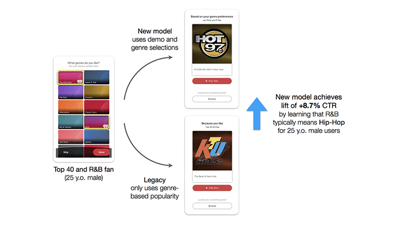
We showed above that our model performed well in offline tests, but we also had to put it to the test in our production app. We tested it by using our model hosted on Amazon SageMaker to recommend a relevant radio station to our new users in the form of an in-app-message directly after registration. We compared this model to business rules that would simply recommend the most popular radio station that was classified into one of the user-selected genres. We ran the A/B test for 10 days with an even split between the groups. The group of users hit with our model predictions had an 8.7% higher click-through rate to the radio station! And of the users who did click, radio listening time was just as strong.

The following diagram shows the real-time predictions result in an 8.7% lift in CTR over the baseline and an example of what the A/B testing groups would have looked like.

Next steps and future work

We’ve shown that new users respond to the relevant content served by our genre prediction model hosted on an Amazon SageMaker endpoint. In our initial proof-of-concept, we introduced the treatment to only a portion of our new registrants. Next steps include expanding this test to a larger user-base and surfacing these recommendations by default in our content carousels for new users with little to no listening history. We also hope to expand the use of these types of models and real-time predictions to other personalization use-cases, such as the ordering of various content carousels and tiles throughout our app. Lastly, we are continuing to explore technologies that allow for seamlessly serving model predictions in real-time including Amazon SageMaker as described in this post as well as others such as FastAPI.

Thanks go out to the Data Science and Data Engineering teams for their support throughout testing the Amazon SageMaker POC and helpful feedback on the post, especially Brett Vintch and Ravi Theja Mudunuru. This post is also available from iHeartMedia on Medium.


About the authors

Matt Fielder is the EVP Engineering at iHeartRadio

Jordan Rosenblum is a Senior Data Scientist at iHeartRadio Digital

Chaining Amazon SageMaker Ground Truth jobs to label progressively

Amazon SageMaker Ground Truth helps you build highly accurate training datasets for machine learning. It can reduce your labeling costs by up to 70% using automatic labeling.

This blog post explains the Amazon SageMaker Ground Truth chaining feature with a few examples and its potential in labeling your datasets. Chaining reduces time and cost significantly as Amazon SageMaker Ground Truth determines the objects that are already labeled and optimizes the data for automated data labeling mode. As a prerequisite, you might want to check the post “Creating hierarchical label taxonomies using Amazon SageMaker Ground Truth” that shows how to achieve multi-step hierarchical labeling and the documentation on how to use the augmented manifest functionality.

Chaining a labeling job

Chaining can help in the following scenarios:

  • Partially completed labeling job – A labeling job in which you have an input manifest that already contains few labels and the rest are to be labeled.
  • Failed labeling job – A labeling job in which you generated a few labels successfully and the rest of the labels either failed or expired.
  • Stopped labeling job – A labeling job that a user stopped, which may have generated a few labels before stopping.

The chaining feature allows you to reuse these previous labels and get the remaining labels coherently. For more information, see Chaining labeling jobs.

Chaining uses the output from a previous job as the input for a subsequent job.

The following are the artifacts used to bootstrap the new chained labeling job:

  1. LabelAttributeName
  2. Output manifest file contents from the previous labeling job
  3. The model, if available

If you are starting a job from the Amazon Sagemaker Ground Truth console, by default, the LabelingJob name is used as the LabelAttributeName. For more information, see LabelAttributeName.

If you are chaining a partially completed job, the console uses the LabelAttributeName of the parent job to decide which object is already labeled and which is not, so that only unlabeled or previously failed objects are sent for labeling. You can override this behavior by providing a different LabelAttributeName, in which case the previous labels aren’t counted and a new labeling job sends all the data for labeling. This post describes this process in more detail later.

If you are using the API or SDK, you need to properly configure these fields, which this post describes later.

When you enable automated data labeling, Amazon Sagemaker Ground Truth uses LabelAttributeName to decide which existing labels to use to start automated data labeling mode and see if you are eligible to train early. You can reap the maximum benefit of machine learning with existing labels; it reduces the cost of labeling tasks because you use existing labels instead of sending them to human labelers again.

Solution overview

The following diagram shows the workflow of this solution.

Step 1: Building the initial unlabeled dataset

Step 2: Launching a labeling job and stopping it (To simulate stopping/Failed status)

Step 3: Chaining your first job

Step 1: Building the initial unlabeled dataset

The first step is to build the initial unlabeled dataset. For more information about this process, see Step 1 in Creating hierarchical label taxonomies using Amazon SageMaker Ground Truth.

This post uses the CBCL StreetScenes dataset, which contains approximately 3547 images. The full dataset is approximately 2 GB; you may choose to upload some or all of the dataset to S3 for labeling. Complete the following steps:

  1. Download the zip file.
  2. Extract the .zip archive to a folder. By default, the folder is Output.
  3. Create a small sample dataset to work with, or use the entire dataset.

For more information about creating an input manifest, see Step 2 in Creating hierarchical label taxonomies using Amazon SageMaker Ground Truth.

The lines in the manifest appear as the following code:

{"source-ref":"s3://bucket_name/datasets/streetscenes/SSDB00001.JPG"}
{"source-ref":"s3://bucket_name/datasets/streetscenes/SSDB00006.JPG"}
{"source-ref":"s3://bucket_name/datasets/streetscenes/SSDB00016.JPG"}
... ...

Step 2: Launching a labeling job and stopping it

From the console, start a labeling job using the Image classification task type to classify pictures as a vehicle, traffic signal, or pedestrian. Use the previously created manifest file as the input and Streetscenes-Job1 as the job name. For more information about starting a labeling job, see Amazon SageMaker Ground Truth – Build Highly Accurate Datasets and Reduce Labeling Costs by up to 70%.

To simulate the stopped or failed state, this post manually stopped the job after 1000 labels.

The output of the labeling job is written to an augmented manifest with the corresponding label augmented in each of the JSON lines in the manifest. Some of these have labels and some do not. See the following code:

1. {
  "source-ref": "s3://bucket_name/datasets/streetscenes/SSDB00001.JPG",
  "Streetscenes-Job1": 0,
  "Streetscenes-Job1-metadata": {
    "confidence": 0.95,
    "job-name": "labeling-job/streetscenes-job1",
    "class-name": "vehicles",
    "human-annotated": "yes",
    "creation-date": "2019-04-09T21:13:37.730999",
    "type": "groundtruth/image-classification"
  }
}
2. {"source-ref":"s3://bucket_name/datasets/streetscenes/SSDB00002.JPG"}
3. {
  "source-ref": "s3://bucket_name/datasets/streetscenes/SSDB00003.JPG",
  "Streetscenes-Job1": 1,
  "Streetscenes-Job1-metadata": {
    "confidence": 0.95,
    "job-name": "labeling-job/streetscenes-job1",
    "class-name": "traffic signals",
    "human-annotated": "yes",
    "creation-date": "2019-04-09T21:25:51.111094",
    "type": "groundtruth/image-classification"
  }
}
4. {"source-ref":"s3://bucket_name/datasets/streetscenes/SSDB00004.JPG"}
5. {"source-ref":"s3://bucket_name/datasets/streetscenes/SSDB00005.JPG"}
6. {"source-ref":"s3://bucket_name/datasets/streetscenes/SSDB00006.JPG"}
7. {"source-ref":"s3://bucket_name/datasets/streetscenes/SSDB00007.JPG"}
8. {
  "source-ref": "s3://bucket_name/datasets/streetscenes/SSDB00008.JPG",
  "Streetscenes-Job1": 0,
  "Streetscenes-Job1-metadata": {
    "confidence": 0.95,
    "job-name": "labeling-job/streetscenes-job1",
    "class-name": "vehicles",
    "human-annotated": "yes",
    "creation-date": "2019-04-09T21:28:54.752427",
    "type": "groundtruth/image-classification"
  }
}
...
...
...

For more information about the format for different modalities, see Output Data.

Step 3: Chaining your first job

You can now chain Streetscenes-Job1. In Labeling jobs, from the Actions dropdown, choose Chain.

The console pre-populates the input dataset location as it fetches the output manifest from the previous stopped job. The label attribute name remains the same as the previous job.

After the job starts, the console shows the counter as 1000, which reflects the data already labeled.

After the job is complete, all labels are generated.

The following code is from the output manifest. All the lines in the output manifest have labels

1. {
  "source-ref": "s3://bucket_name/datasets/streetscenes/SSDB00006.JPG",
  "Streetscenes-Job1": 3,
  "Streetscenes-Job1-metadata": {
    "confidence": 0.59,
    "job-name": "labeling-job/streetscenes-job1-chain",
    "class-name": "None",
    "human-annotated": "yes",
    "creation-date": "2019-04-10T01:37:07.663801",
    "type": "groundtruth/image-classification"
  }
}

2. {
  "source-ref": "s3://bucket_name/datasets/streetscenes/SSDB00007.JPG",
  "Streetscenes-Job1": 0,
  "Streetscenes-Job1-metadata": {
    "job-name": "labeling-job/streetscenes-job1-chain",
    "confidence": 0.99,
    "class-name": "vehicles",
    "type": "groundtruth/image-classification",
    "creation-date": "2019-04-10T01:23:05.309990",
    "human-annotated": "no"
  }
}

...

Chaining in a series

The previous scenarios only showed one level of chaining. Chaining is a powerful feature in which you can feed the output of one job as input to another.

Scenarios for chaining

The following table shows some of the scenarios with which you can experiment with chaining. AL indicates that automated data labeling mode is enabled. Non-AL indicates that automated data labeling mode is not enabled. For more information, see Annotate data for less with Amazon SageMaker Ground Truth and automated data labeling.

Parent labeling job Chained labeling lob Details
1 Non-AL Non-AL You started a labeling job in Non-AL mode and it failed or stopped before labeling all the objects. You want to resume the job in Non-AL mode to label the remaining unlabeled objects by a human.
2 Non-AL AL You started a labeling job in Non-AL mode and it failed or stopped before labeling all the objects. You want to resume the job in AL mode to label the remaining unlabeled objects automatically based on the existing labels.
3 AL Non-AL You started a labeling job in AL mode and it failed or stopped before labeling all the objects. You want to resume the job in Non-AL mode to label the remaining unlabeled objects by a human.
4 AL AL You started a labeling job in AL mode and it failed or stopped before labeling all the objects. You want to resume the job in AL mode to label the remaining unlabeled objects automatically based on the existing labels or pre-trained models.
5 Third-Party labels Non-AL You acquired some labels through other sources (Amazon SageMaker Ground Truth or a third party) and have a manifest with labeled objects and unlabeled data. You want to start a new job in Non-AL mode to label the remaining unlabeled objects automatically based on the existing labels.
6 Third-Party labels AL You acquired some labels through other sources (Amazon SageMaker Ground Truth or a third party) and have a manifest with labeled objects and unlabeled data. You want to start a new job in AL mode to label the remaining unlabeled objects automatically based on the existing labels.

In some of these scenarios, if you are in AL mode and the job stops after a model is generated, the subsequent AL job uses the model from the first step, which reduces training time. For more information, see Amazon SageMaker Ground Truth: Using a Pre-Trained Model for Faster Data Labeling.

Additionally, if enough pre-labeled objects are available, you can bootstrap these labels to be the training set for your automated labeling loop. This method saves on time and cost by not fetching labels from human annotators.

Using third-party labels

This section elaborates on the final two scenarios in the previous table. You can bring in third-party labels as long as it adheres to the Amazon Sagemaker Ground Truth label format. For more information, see Output Data.

For example, assume you have a job in which the manifest has 989/3450 third-party labels. You can start the labeling job with the following code, which contains third-party labels:

{
  "source-ref": "s3://bucket-name/datasets/streetscenes/SSDB03295.JPG",
  "third-party-label": 0,
  "third-party-label-metadata": {
    "confidence": 0.95,
    "job-name": "labeling-job/third-party-label",
    "class-name": "vehicles",
    "human-annotated": "yes",
    "creation-date": "2019-04-09T21:25:51.110794",
    "type": "groundtruth/image-classification"
  }
}
...

After the job starts, it automatically updates the counter.

Time and cost savings

Chaining offers many time- and cost-saving benefits.

Firstly, objects that are already labeled aren’t processed again. Additionally, if automated data labeling is enabled, auto labeling is attempted as soon as possible. If your data is already partially labeled, a validation set is collected by sending work to a human workforce, after which you can bootstrap the partially labeled input data to be the training set, and Amazon Sagemaker Ground Truth performs automated labeling depending on the number of existing labels. This expedites the automated data labeling process; training starts sooner and reduces the training job’s overall time.

Furthermore, skipping labeled objects reduces costs. Training costs are also reduced by using the ML model generated from your existing data.

Chaining using the API

You can also use the API or AWS CLI to do chaining. For more information, see create-labeling-job.

If you have a failed job and want to resume it, you need to enter the same create-labeling-job information as the failed job, with the same LabelAttributeName as the previous job, and use the output manifest file as the input in your chained job.

Similarly, if you want to chain the job for labeling all the objects with a different kind of label, you need to use a different LabelAttributeName than the one in the previous labeling job.

The following code is an example CLI for chaining:

>> aws sagemaker create-labeling-job --labeling-job-name "Streetscenes-Job1-chain" --label-attribute-name "Streetscenes-Job1" --input-config DataSource={S3DataSource={ManifestS3Uri="s3://<bucket_name>/streetscenes/output/Streetscenes-Job1/manifests/output/output.manifest"}},DataAttributes={ContentClassifiers=["FreeOfPersonallyIdentifiableInformation"]} --output-config S3OutputPath="s3://<bucket_name>/streetscenes/output/Streetscenes-Job1-chain/" --role-arn "arn:aws:iam::accountID:role/<rolename>" --label-category-config-s3-uri "s3://<path_to_label_category_file>/labelcategory.json" --stopping-conditions MaxPercentageOfInputDatasetLabeled=100 --human-task-config WorkteamArn="arn:aws:sagemaker:region:394669845002:workteam/public-crowd/default",UiConfig={UiTemplateS3Uri="s3://<bucket_name>/template.liquid"},PreHumanTaskLambdaArn="arn:aws:lambda:us-west-2:081040173940:function:PRE-ImageMultiClass",TaskKeywords="Images","classification",TaskTitle="Image Categorization",TaskDescription="Categorize images into specific classes",NumberOfHumanWorkersPerDataObject=3,TaskTimeLimitInSeconds=300,TaskAvailabilityLifetimeInSeconds=21600,MaxConcurrentTaskCount=1000,AnnotationConsolidationConfig={AnnotationConsolidationLambdaArn="arn:aws:lambda:us-west-2:081040173940:function:ACS-ImageMultiClass"}

This code uses the same label attribute name (label-attribute-name) as the first job, Streetscenes-Job1.

Conclusion

This post demonstrated how the Amazon SageMaker Ground Truth chaining feature offers time-saving and cost-reduction benefits. This is a very powerful feature and this post merely scratches the surface of what Amazon SageMaker Ground Truth chaining can do. Let us know what you think in the comments. You can get started with Amazon Sagemaker Ground Truth by visiting Getting Started page in the documentation.


About the authors

Priyanka Gopalakrishna is a software engineer at Amazon AI. She works on building scalable solutions using distributed systems for machine learning. In her spare time, she loves to hike, catch up on things related to space sciences or read good old strips of Calvin and Hobbes.


Zahid Rahman is a SDE in AWS AI where he builds large scale distributed systems to solve complex machine learning problems . He is primarily focused on innovating technologies that can ‘Divide and Conquer’ Big Data problem.

Subtitling videos accurately and easily with CaptionHub and AWS

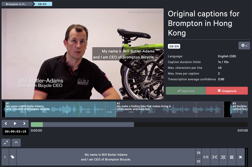
This is a guest post from James Jameson, the Commercial Lead at CaptionHub. CaptionHub is a London-based company that focuses on video captioning and subtitling production for enterprise organizations.

While the act of captioning—that is, taking video files and making sure the text on the screen reflects what’s being said accurately and is timed appropriately—seems simple at the outset, there is more complexity than meets the eye.

When we embarked on building CaptionHub in 2015, we were a design agency producing video effects and commercials for clients, including a massive tech company in California. They wanted us to localize their video—to their high standards, of course—and do it on the tight schedule of a global consumer tech release.

To meet our client’s needs, we found ourselves building a new software tool to manage linguists, provide collaborative subtitling, and make subtitles frame-accurate. To speed up the process, we then added AI called Natural Captions Technology, an algorithmic approach to natural language processing that reflects the natural language of humans.

From this starting point, we recognized the ubiquitous needs for a solution like what we had created. We broadened the types of media we handled from simply marketing or internal communications assets to high-value global output ready for any viewer or listener worldwide.

With CaptionHub today, we take recorded video and create perfect subtitles, fast. We generate subtitles using automatic speech recognition to massively speed up the first cut. Then, we make sure that subtitles are timed perfectly (“frame-accurate,” in our lingo), on the belief that subtitling should be a seamless part of the production workflow. We also provide automated and human-enabled translation to localize video for any audience. Now, with the help of AWS, we can do that for live video streams and on-demand video.

With AWS, we can provide an enterprise localization platform for the most demanding of our clients, regardless of their use case. AWS technology spans our servers and low-level infrastructure decisions up to the engines we choose for speech recognition, machine translation, and the sharp-end value points that delight our customers.

On the artificial intelligence and machine learning side, we use Amazon Translate and Amazon Transcribe for smooth, real-time captioning across dozens of languages. AWS has been a crucial inspiration for our newest offerings.

We use a variety of other AWS services that are critical to our infrastructure and application architecture. AWS Elemental MediaPackage handles output streams from CaptionHub live, combining captions and video/audio, while AWS Elemental MediaLive handles the input streams for CaptionHub live. While all of this is orchestrated in perfect harmony, we use Amazon CloudWatch to monitor our AWS infrastructure.

With this AWS-based setup, we’re unstoppable. We’re able to scale up and down however and whenever we need to. AWS has allowed us to vastly accelerate our mission to help organizations localize their media.

Our customers have reported huge savings in workflow time, up to an 800% increase in production for captions and subtitles using automatic speech recognition, which takes advantage of the same tech behind Alexa. That amounts to a significant financial return, even for the world’s largest and best-funded production and marketing departments.

We live in a world that communicates with video. When our clients’ production values, combined with their potential to reach audiences, quite literally define their brand, it’s no wonder they want to maintain that winning edge. With CaptionHub’s captioning solutions, made possible by AWS, we can ensure that organizations reach audiences in their language, quickly and perfectly, on any device, wherever they are.

Exploring images on social media using Amazon Rekognition and Amazon Athena

If you’re like most companies, you wish to better understand your customers and your brand image. You’d like to track the success of your marketing campaigns, and the topics of interest—or frustration—for your customers. Social media promises to be a rich source of this kind of information, and many companies are beginning to collect, aggregate, and analyze the information from platforms like Twitter.

However, more and more social media conversations center around images and video; on one recent project, approximately 30% of all tweets collected included one or more images. These images contain relevant information that is not readily accessible without analysis.

About this blog post
Time to complete 1 hour
Cost to complete ~ $5 (at publication time, depending on terms used)
Learning level Intermediate (200)
AWS services Amazon Rekognition
Amazon Athena
Amazon Kinesis Data Firehose
Amazon S3
AWS Lambda

Overview of solution

The following diagram shows the solution components and how the images and extracted data flows through them.

These components are available through an AWS CloudFormation template.

  1. Twitter Search API collects Tweets.
  2. Amazon Kinesis Data Firehose dispatches the tweets to store in an Amazon S3
  3. The creation of an S3 object in the designated bucket folder triggers a Lambda function.
  4. The Lambda sends each tweet text to Amazon Comprehend to detect sentiment (positive or negative), entity (real-world objects such as people, places, and commercial items), and to precise references to measures such as dates and quantities. For more information, see DetectSentiment and DetectEntity in the Amazon Comprehend Developer Guide.
  5. The Lambda checks each tweet for media of type ‘photo’ in the tweet’s extended_entities If the photo has either a .JPG or .PNG extension, the Lambda calls the following Amazon Rekognition APIs for each image:
    • Detect_labels, to identify objects such as Person, Pedestrian, Vehicle, and Car in the image.
    • Detect_moderation_labels, to determine if an image or stored video contains unsafe content, such as explicit adult content or violent content.
    • If the detect_labels API returns a Text label, detect_text extracts lines, words, or letters found in the image.
    • If the detect_labels API returns a Person label, the Lambda calls the following:
      • detect_faces, to detect faces and analyze them for features such as sunglasses, beards, and mustaches.
      • recognize_celebrities, to detect as many celebrities as possible in different settings, cosmetic makeup, and other conditions.

      The results from all calls for a single image are combined into a single JSON record. For more information about these APIs, see Actions in the Amazon Rekognition Developer Guide.

  6. The results of the Lambda go to Kinesis Data Firehose. Kinesis Data Firehose batches the records and writes them to a designated S3 bucket and folder.
  7. You can use Amazon Athena to build tables and views over the S3 datasets, then catalogue these definitions in the AWS Glue Data Catalog. The table and view definitions make it much easier to query the complex JSON objects contained in these S3 datasets.
  8. After the processed tweets land in S3, you can query the data with Athena.
  9. You can also use Amazon QuickSight to visualize the data, or Amazon SageMaker or Amazon EMR to process the data further. For more information, see Build a social media dashboard using machine learning and BI services. This post uses Athena.

Prerequisites

This walkthrough has the following prerequisites:

  • An AWS account.
  • An app on Twitter. To create an app, see the Apps section of the Twitter Development website.
    • Create a consumer key (API key), consumer secret key (API secret), access token, and access token secret. The solution uses them as parameters in the AWS CloudFormation stack.

Walkthrough

This post walks you through the following steps:

  • Launching the provided AWS CloudFormation template and collecting tweets.
  • Checking that the stack created datasets on S3.
  • Creating views over the datasets using Athena.
  • Exploring the data.

S3 stores the raw tweets and the Amazon Comprehend and Amazon Rekognition outputs in JSON format. You can use Athena table and view definitions to flatten the complex JSON produced and extract your desired fields. This approach makes the data easier to access and understand.

Launching the AWS CloudFormation template

This post provides an AWS CloudFormation template that creates all the ingestion components that appear in the previous diagram, except for the S3 notification for Lambda (the dotted blue line in the diagram).

  1. In the AWS Management Console, launch the AWS CloudFormation Template.

    This launches the AWS CloudFormation stack automatically into the us-east-1 Region.

  2. In the post Build a social media dashboard using machine learning and BI services, in the section “Build this architecture yourself,” follow the steps outlined, with the following changes:
    • Use the Launch Stack link from this post.
    • If the AWS Glue database socialanalyticsblog already exists (for example, if you completed the walkthrough from the previous post), change the name of the database when launching the AWS CloudFormation stack, and use the new database name for the rest of this solution.
    • For Twitter Languages, use ‘en’ (English) only. This post removed the Amazon Comprehend Translate capability for simplicity and to reduce cost.
    • Skip the section “Setting up S3 Notification – Call Amazon Translate/Comprehend from new Tweets.” This occurs automatically when launching the AWS CloudFormation stack by the “Add Trigger” Lambda function.
    • Stop at the section “Create the Athena Tables” and complete the following instructions in this post instead.

You can modify which terms to pull from the Twitter streaming API to be those relevant for your company and your customers. This post used several Amazon-related terms.

This implementation makes two Amazon Comprehend calls and up to five Amazon Rekognition calls per tweet. The cost of running this implementation is directly proportional to the number of tweets you collect. If you’d like to modify the terms to something that may retrieve tens or hundreds of tweets a second, for efficiency and for cost management, consider performing batch calls or using AWS Glue with triggers to perform batch processing versus stream processing.

Checking the S3 files

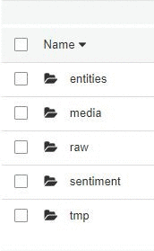
After the stack has been running for approximately five minutes, datasets start appearing in the S3 bucket (rTweetsBucket) that the AWS CloudFormation template created. Each dataset is represented as the following files sitting in a separate directory in S3:

  • Raw – The raw tweets as received from Twitter.
  • Media – The output from calling the Amazon Rekognition APIs.
  • Entities – The results of Amazon Comprehend entity analysis.
  • Sentiment – The results of Amazon Comprehend sentiment analysis.

See the following screenshot of the directory:
For the entity and sentiment tables, see Build a social media dashboard using machine learning and BI services.

When you have enough data to explore (which depends on how popular your selected terms are and how frequently they have images), you can stop the Twitter stream producer, and stop or terminate the Amazon EC2 instance. This stops your charges from Amazon Comprehend, Amazon Rekognition, and EC2.

Creating the Athena views

The next step is manually creating the Athena database and tables. For more information, see Getting Started in the Athena User Guide.

This is a great place to use AWS Glue crawling features in your data lake architectures. The crawlers automatically discover the data format and data types of your different datasets that live in S3 (as well as relational databases and data warehouses). For more information, see Defining Crawlers.

  1. In the Athena console, in Query Editor, access the file sql.The AWS CloudFormation stack created the database and tables for you automatically.
  2. Load the view create statements into the Athena query editor one by one, and execute.This step creates the views over the tables.

Compared to the prior post, the media_rekognition table and the views are new. The tweets table has a new extended_entities column for images and video metadata. The definitions of the other tables remain the same.

Your Athena database should look similar to the following screenshot. There are four tables, one for each of the datasets on S3. There are also three views, combining and exposing details from the media_rekognition table:

  • Celeb_view focuses on the results of the recognize_celebrities API
  • Media_image_labels_query focuses on the results from the detect_labels API
  • Media_image_labels_face_query focuses on the results from the detect_faces API

Explore the table and view definitions. The JSON objects are complex, and these definitions show a variety of uses for querying nested objects and arrays with complex types. Now many of the queries can be relatively simple, thanks to the underlying table and view definitions encapsulating the complexity of the underlying JSON. For more information, see Querying Arrays with Complex Types and Nested Structures.

Exploring the results

This section describes three use cases for this data and provides SQL to extract similar data. Because your search terms and timeframe are different from those in this post, your results will differ. This post used a set of Amazon-related terms. The tweet collector ran for approximately six weeks and collected approximately 9.5M tweets. From the tweets, there were approximately 0.5M photos, about 5% of the tweets. This number is low compared to some other sets of business-related search terms, where approximately 30% of tweets contained photos.

This post reviews for four image use cases:

  1. Buzz
  2. Labels and faces
  3. Suspect content
  4. Exploring celebrities

Buzz

Major topic areas represented by the links associated with the tweets often provide a good complement to the tweet language content topics surfaced via natural language processing. For more information, see Build a social media dashboard using machine learning and BI services.

The first query is which websites the tweets linked to. The following code shows the top domain names linked from the tweets:

SELECT lower(url_extract_host(url.expanded_url)) AS domain,
         count(*) AS count
FROM 
    (SELECT *
    FROM "tweets"
    CROSS JOIN UNNEST (entities.urls) t (url))
GROUP BY  1
ORDER BY  2 DESC 
LIMIT 10;

The following screenshot shows the top 10 domains returned:

Links to Amazon websites are frequent, and several different properties are named, such as amazon.com, amazon.co.uk, and goodreads.com.

Further exploration shows that many of these links are to product pages on the Amazon website. It’s easy to recognize these links because they have /dp/ (for detail page) in the link. You can get a list of those links, the images they contain, and the first line of text in the image (if there is any), with the following query:

SELECT tweetid,
         user_name,
         media_url,
         element_at(textdetections,1).detectedtext AS first_line,
         expanded_url,
         tweet_urls."text"
FROM 
    (SELECT id,
         user.name AS user_name,
         text,
         entities,
         url.expanded_url as expanded_url
    FROM tweets
    CROSS JOIN UNNEST (entities.urls) t (url)) tweet_urls
JOIN 
    (SELECT media_url,
         tweetid,
         image_labels.textdetections AS textdetections
    FROM media_rekognition) rk
    ON rk.tweetid = tweet_urls.id
WHERE lower(url_extract_host(expanded_url)) IN ('www.amazon.com', 'amazon.com', 'www.amazon.com.uk', 'amzn.to')
        AND NOT position('/dp/' IN url_extract_path(expanded_url)) = 0 -- url links to a product
LIMIT 50;

The following screenshot shows some of the records returned by this query. The first_line column shows the results returned by the detect_text API for the image URL in the media_url column.

Many of the images do contain text. You can also identify the products the tweet linked to; many of the tweets are product advertisements by sellers, using images that relate directly to their product.

Labels and faces

You can also get a sense of the visual content of the images by looking at the results of calling the Amazon Rekognition detect_labels API. The following query finds the most common objects found in the photos:

SELECT label_name,
         COUNT(*) AS count
FROM media_image_labels_query
GROUP BY  label_name
ORDER BY COUNT(*) desc
LIMIT 50; 

The following screenshot shows the results of that request. The most popular label by far is Human or Person, with Text, Advertisement, and Poster coming soon after. Novel is further down the list. This result reflects the most popular product being tweeted about on the Amazon website—books.

You can explore the faces further by looking at the results of the detect_faces API. That API returns details for each face in the image, including the gender, age range, face position, whether the person is wearing sunglasses or has a mustache, and the expression(s) on their face. Each of these features also has a confidence level associated with it. For more information, see DetectFaces in the Amazon Rekognition Developer Guide.

The view media_image_labels_face_query unnests many of these features from the complex JSON object returned by the API call, making the fields easy to access.

You can explore the view definition for media_image_labels_face_query, including the use of the reduce operator on the array of (emotion,confidence) pairs that Amazon Rekognition returned to identify and return the expression category with the highest confidence score associated with it, and associate the name top_emotion with it. See the following code:

reduce(facedetails.emotions, element_at(facedetails.emotions, 1), (s_emotion, emotion) -> IF((emotion.confidence > s_emotion.confidence), emotion, s_emotion), (s) -> s) top_emotion

You can then use the exposed field, top_emotion. See the following code:

SELECT top_emotion.type AS emotion ,
         top_emotion.confidence AS emotion_confidence ,
         milfq.* ,   
         "user".id AS user_id ,
         "user".screen_name ,
         "user".name AS user_name ,
        url.expanded_url AS url
FROM media_image_labels_face_query milfq
INNER JOIN tweets
    ON tweets.id = tweetid, UNNEST(entities.urls) t (url)
WHERE position('.amazon.' IN url.expanded_url) > 0;

The following screenshot shows columns from the middle of this extensive query, including glasses, age range, and where the edges of this face are positioned. This last detail is useful when multiple faces are present in a single image, to distinguish between the faces.

You can look at the top expressions found on these faces with the following code:

SELECT top_emotion.type AS emotion,
         COUNT(*) AS "count"
FROM media_image_labels_face_query milfq
WHERE top_emotion.confidence > 50
GROUP BY top_emotion.type
ORDER BY 2 desc; 

The following screenshot of the query results shows that CALM is the clear winner, followed by HAPPY. Oddly, there are far fewer confused than disgusted expressions.

Suspect content

A topic of frequent concern is whether there is content in the tweets, or the associated images, that should be moderated. One of the Amazon Rekognition APIs called by the Lambda for each image is moderation_labels, which returns labels denoting the category of content found, if any. For more information, see Detecting Unsafe Content.

The following code finds tweets with suspect images. Twitter also provides a possibly_sensitive flag based solely on the tweet text.

SELECT tweetid,
    possibly_sensitive, 
transform(image_labels.moderationlabels, ml -> ml.name) AS moderationlabels, 
"mediaid", "media_url" , 
tweets.text, 
"url"."expanded_url" AS url , 
    (CASE WHEN ("substr"("tweets"."text", 1, 2) = 'RT') THEN
    true
    ELSE false END) "isretweet"
FROM media_rekognition
INNER JOIN tweets
    ON ("tweets"."id" = "tweetid"), UNNEST("entities"."urls") t (url)
WHERE cardinality(image_labels.moderationlabels) > 0
        OR possibly_sensitive = True;

The following screenshot shows the first few results. For many of these entries, the tweet text or the image may contain sensitive content, but not necessarily both. Including both criteria provides additional safety.

Note the use of the transform construct in the preceding query to map over the JSON array of moderation labels that Amazon Rekognition returned. This construct lets you transform the original content of the moderationlabels object (in the following array) into a list containing only the name field:

[{confidence=52.257442474365234, name=Revealing Clothes, parentname=Suggestive}, {confidence=52.257442474365234, name=Suggestive, parentname=}]  

You can filter this query to focus on specific types of unsafe content by filtering on specific moderation labels. For more information, see Detecting Unsafe Content.

A lot of these tweets have product links embedded in the URL. URLs for the Amazon.com website have a pattern to them: any URL with /dp/ in it is a link to a product page. You could use that to identify the products that may have explicit content associated with them.

Exploring celebrities

One of the Amazon Rekognition APIs that the Lambda called for each image was recognize_celebrity. For more information, see Recognizing Celebrities in an Image.

The following code helps determine which celebrities appear most frequently in the dataset:

SELECT name as celebrity,
         COUNT (*) as count
FROM celeb_view
GROUP BY  name
ORDER BY  COUNT (*) desc;

The result counts instances of celebrity recognitions, and counts an image with multiple celebrities multiple times.

For example, assume there is a celebrity with the label JohnDoe. To explore their images further, use the following query. This query finds the images associated with tweets in which JohnDoe appeared in the text or the image.

SELECT cv.media_url,
         COUNT (*) AS count ,
         detectedtext
FROM celeb_view cv
LEFT JOIN      -- left join to catch cases with no text 
    (SELECT tweetid,
         mediaid,
         textdetection.detectedtext AS detectedtext
    FROM media_rekognition , UNNEST(image_labels.textdetections) t (textdetection)
    WHERE (textdetection.type = 'LINE'
            AND textdetection.id = 0) -- get the first line of text
    ) mr
    ON ( cv.mediaid = mr.mediaid
        AND cv.tweetid = mr.tweetid )
WHERE ( ( NOT position('johndoe' IN lower(tweettext)) = 0 ) -- JohnDoe IN text
        OR ( (NOT position('johndoe' IN lower(name)) = 0) -- JohnDoe IN image
AND matchconfidence > 75) )  -- with pretty good confidence
GROUP BY  cv.media_url, detectedtext
ORDER BY  COUNT(*) DESC;

The recognize_celebrity API matches each image to the closest-appearing celebrity. It returns that celebrity’s name and related information, along with a confidence score. At times, the result can be misleading; for example, if a face is turned away, or when the person is wearing sunglasses, they can be difficult to identify correctly. In other instances, the API may choose an image model because of their similarity to a celebrity. It may be beneficial to combine this query with logic using the face_details response, to check for glasses or for face position.

Cleaning up

To avoid incurring future charges, delete the AWS CloudFormation stack, and the contents of the S3 bucket created.

Conclusion

This post showed how to start exploring what your customers are saying about you on social media using images. The queries in this post are just the beginning of what’s possible. To better understand the totality of the conversations your customers are having, you can combine the capabilities from this post with the results of running natural language processing against the tweets.

This entire processing, analytics, and machine learning pipeline—starting with Kinesis Data Firehose, using Amazon Comprehend to perform sentiment analysis, Amazon Rekognition to analyze photographs, and Athena to query the data—is possible without spinning up any servers.

This post added advanced machine learning (ML) services to the Twitter collection pipeline, through some simple calls within Lambda. The solution also saved all the data to S3 and demonstrated how to query the complex JSON objects using some elegant SQL constructs. You could do further analytics on the data using Amazon EMR, Amazon SageMaker, Amazon ES, or other AWS services. You are limited only by your imagination.


About the authors

Dr. Veronika Megler is Principal Consultant, Data Science, Big Data & Analytics, for AWS Professional Services. She holds a PhD in Computer Science, with a focus on scientific data search. She specializes in technology adoption, helping companies use new technologies to solve new problems and to solve old problems more efficiently and effectively.


Chris Ghyzel is a Data Engineer for AWS Professional Services. Currently, he is working with customers to integrate machine learning solutions on AWS into their production pipelines. 


Adding AI to your applications with ready-to-use models from AWS Marketplace

Machine learning (ML) lets enterprises unlock the true potential of their data, automate decisions, and transform their business processes to deliver exponential value to their customers. To help you take advantage of ML, Amazon SageMaker provides the ability to build, train, and deploy ML models quickly.

Until recently, if you used Amazon SageMaker, you could either choose optimized algorithms offered in Amazon SageMaker or bring your own algorithms and models. AWS Marketplace for Machine Learning increases the selection of ML algorithms and models. You can choose from hundreds of free or paid algorithms and model packages across a broad range of categories, including:

In this post, you learn how to deploy and perform inference on the Face Anonymizer model package from the AWS Marketplace for Machine Learning.

Overview

Model packages in AWS Marketplace are pre-trained machine learning models that can be used to perform batch as well as real-time inference. Because these model packages are pre-trained, you don’t have to worry about any of the following tasks:

  • Gathering training data
  • Writing an algorithm for training a model
  • Performing hyperparameter-optimization
  • Training a model and getting it ready for production

Not having to do these steps saves you much time and money spent writing algorithms, finding datasets, feature engineering, and training and tuning the model.

Algorithms and model packages from AWS Marketplace integrate seamlessly with Amazon SageMaker. To interact with them, you can use the AWS Management Console, the low-level Amazon SageMaker API, or the Amazon SageMaker Python SDK. You can use model packages to either stand up an Amazon SageMaker endpoint for performing real-time inference or run a batch transform job.

Amazon SageMaker provides a secure environment to use your data with third-party software. You are recommended to follow principle of least privilege and ensure that IAM permissions are locked down for your resources.

To be able to try this blogpost successfully, you would need appropriate IAM permissions. For Amazon SageMaker IAM permissions and best practices to be followed, see documentation. For more information how to secure your machine learning workloads, watch an online tech talk on Building Secure Machine Learning Environments Using Amazon SageMaker. The service helps you secure your data in multiple ways::

  • Amazon SageMaker performs static and dynamic scans of all the algorithms and model packages for vulnerabilities to ensure data security.
  • Amazon SageMaker encrypts algorithm and model artifacts and other system artifacts in transit and at rest.
  • Requests to the Amazon SageMaker API and the console are made over a secure (HTTPS over TLS) connection.
  • Amazon SageMaker requires IAM credentials to access resources and data on your deployment, thus preventing the seller’s access to your data.
  • Amazon SageMaker isolates the deployed algorithm/model artifacts from internet access to secure your data. For more information, see Training and Inference Containers Run in Internet-Free Mode.

Walkthrough

There are many different reasons why you may want to blur faces for the reasons of ensuring anonymity and privacy.  As a developer, you want to add intelligence to your automation process without having to worry about training a model.

After searching for pre-trained ML models on the internet, you come across AWS Marketplace for Machine Learning. A Search for the keyword “face” results in a list of algorithms. You decide to try the Face Anonymizer model package by Figure Eight.

Before you deploy the model, you need to review the AWS Marketplace listing to understand the I/O interface of the model package and its pricing information. Open the listing and review the product overview, pricing, highlights, usage information, instance types with which the listing is compatible, and additional resources. To deploy the model, your AWS account must have a subscription to it.

Subscribe to the model package

On the listing page, choose Continue to Subscribe. Review the End User license agreement and software pricing and once your organization agrees to the same, Accept offer button needs to be clicked.

    • For AWS Marketplace IAM permissions,  see “Rule 1 Only those users who are authorized to accept a EULA on behalf of your organization should be allowed to procure (or subscribe to) a product in Marketplace” from my other blog post, Securing access to AMIs in AWS Marketplace.

Create a deployable model

After subscription to the listing has been made from your AWS account, you can deploy the model package:

  1. Open configure your software page for Face Anonymizer. Leave Fulfillment method as Amazon SageMaker and Software Version as Version 1. For Region, choose us-east-2. At the bottom of the page is Product ARN, which is required only if you deploy the model using the API. Because you are deploying Amazon SageMaker Endpoint using the console, you can ignore it.
  2. Choose View in SageMaker.
  3. Select the Face Anonymizer listing and then choose Create endpoint.
  4. Under Model settings section, specify the following parameters and then choose NEXT:
    1. Specify face-anonymizer for Model name.
    2. For IAM role, select an IAM role that has necessary IAM permissions.

    You just used a pre-trained model package from AWS Marketplace to create a deployable model. A deployable model has an IAM role associated with it while the model package is a static entity and does not have an IAM role associated with it. Next, you deploy the model to perform inference.

Deploy the model

  1. On the Create Endpoint page, configure the following fields:
    1. For Endpoint name & Endpoint configuration name, choose face-anonymizer.
    2. Under Production variants, choose Edit.
  2. In the Edit Production Variant dialog box, configure the following fields:
    1. For instance type, select ml.c5.xlarge (the Face Anonymizer listing is compatible with ml.c5.xlarge as the instance type)
    2. Choose Save.
  3. Review the information as shown in the following screenshot and choose Create endpoint configuration.
  4. Choose Submit to create the endpoint.

Perform inference on the model

Each model package from AWS Marketplace has a specific input format, which is in its listing, in the Usage Information section. For example, the listing for Face Anonymizer states that the input must be base64-encoded and the payload sent for prediction should be in the following format:

Payload: 
{
	"instances": [{
		"image": {
			"b64": "BASE_64_ENCODED_IMAGE_CONTENTS"
		}
	}]
}

For this post, use the following image with the file name volunteers.jpg to perform anonymization.

The following section contains commands you can use from terminal to prepare data and to perform inference.

Perform base64-encoding

Since the payload required needs to be base64 encoded to perform real-time inference, you must first encode the image.

Linux command

encoded_string=$(base64 volunteers.jpg)

Windows – PowerShell commands

$base64string = [Convert]::ToBase64String([IO.File]::ReadAllBytes('./volunteers.jpg'))

Prepare payload

Use following commands to prepare the payload and write it to a file.

Linux commands

payload="{"instances": [{"image": {"b64": "$encoded_string"}}]}"
echo $payload >input.json

Windows – PowerShell commands

$payload=-join('{"instances": [{"image": {"b64": "' ,$base64string,'"}}]}')

$Utf8NoBomEncoding = New-Object System.Text.UTF8Encoding $False

 [System.IO.File]::WriteAllLines('./input.json', $payload, $Utf8NoBomEncoding)

Now that the payload is ready, you can either perform a batch inference or a real-time inference.

Perform real-time inference

To perform real-time inference, execute the following command using the AWS CLI. For more information, see Installing the AWS CLI and Configuring the AWS CLI.

aws sagemaker-runtime invoke-endpoint --endpoint-name face-anonymizer --body fileb://input.json --content-type "application/json" --region us-east-2 output.json.out

After you execute the command, the output is available in the output.json.out file.

Perform batch inference

To perform a batch inference:

  1. Sign in to the AWS Management Console. Then you can either identify an Amazon S3 bucket to use, or create an S3 bucket in the same Region in which you deployed the model earlier.
  2. Upload the input.json file to the S3 bucket.
  3. To copy the path of the file, select the file and choose Copy Path.
  4. In the Amazon SageMaker console, choose Batch Transform Jobs, Create Batch Transform Job.
  5. Specify the following information and choose Create Job.
    1. For Job name, enter face-anonymization.
    2. For Model name, enter face-anonymizer.
    3. For Instance type, select c5.xlarge.
    4. For Instance-count, enter 1.
    5. Under Input data configuration, for S3 location, specify the S3 path that you copied. It should look like the following pattern:
      s3://<your-bucket-name>/input.json 

    6. For Content type, enter application/json.
    7. For Output data configuration, specify the appropriate S3 output path. It should look like this:
      s3://<your-bucket-name>/output

  1. A message appears stating that a batch transform job was successfully created. After the status of the job changes to Completed, open the batch transform job, under Output data configuration, select output data path, and then download the output file with name json.out.

Extract and visualize the output

Now that the output is available, you can extract it using the commands in the following chart and visualize the output.

Linux command

cat output.json.out | jq -r '.predictions[0].image.b64' | base64 --decode >output.jpg

Windows – PowerShell commands

$jsondata = Get-Content -Raw -Path 'output.json.out' | ConvertFrom-Json

$bytes = [Convert]::FromBase64String($jsondata.predictions.image.b64)

[IO.File]::WriteAllBytes('output.jpg', $bytes)

In the output.jpg image, you can see that the ML model identified and anonymized the faces in the image.

You successfully performed a real-time inference on a model created from a third-party model package from AWS Marketplace.

Cleaning up

Delete the endpoint and the endpoint configuration so that your account is no longer charged.

  1. To delete the endpoint:
    1. In the Amazon SageMaker console, choose Endpoints.
    2. Select the endpoint with the name face-anonymizer and choose Actions, Delete.
  2. To delete the endpoint configuration:
    1. In the Amazon SageMaker console, choose Endpoint configuration.
    2. Select the endpoint configuration with the name face-anonymizer and choose Actions, Delete.
  3. To delete the model;
    1. In the Amazon SageMaker console, choose Models.
    2. Select the model with the name face-anonymizer and choose Actions, Delete.
  4. If you subscribed to the listing simply to try the example in this post, you can unsubscribe to the listing. On the Your software subscriptions page, choose Cancel Subscription for the Face Anonymizer listing.

Deploy a model and perform real-time and batch inference using a Jupyter notebook

This post demonstrated how to use the Amazon SageMaker console to stand up an Amazon SageMaker endpoint and use the AWS CLI to perform inference. If you prefer to try a model package using a Jupyter notebook, use the following steps:

  1. Create an Amazon SageMaker notebook instance.
  2. In the Amazon SageMaker console, under Notebook instances, in the Actions column for the notebook instance that you just created, choose Open Jupyter.
  3. In the notebook, choose SageMaker Examples.
  4. Under AWS Marketplace, choose Use for the “Using_ModelPackage_Arn_From_AWS_Marketplace.ipynb” sample notebook available, and then follow the notebook. Use Shift+Enter to run each cell.

Pricing

AWS Marketplace contains the following pricing for model packages:

  • Free (no software pricing)
  • Free-trial (no software pricing for a limited trial period)
  • Paid

Apart from infrastructure costs, the Free-trial and Paid model packages have software pricing applicable for real-time Amazon SageMaker inference and Amazon SageMaker batch transform. You can find this information on the AWS Marketplace listing page in the Pricing Information section. Software pricing for third-party model packages may vary based on Region, instance type, and inference type.

Conclusion

This post took you through a use case and provided step-by-step instructions to start performing predictions on ML models created from third-party model packages from AWS Marketplace.

In addition to third-party model packages, AWS Marketplace also contains algorithms. These can be used to train a custom ML model by creating a training job or a hyperparameter tuning job. With third-party algorithms, you can choose from a variety of out-of-the-box algorithms. By reducing the time-to-deploy by eliminating algorithm development efforts, you can focus on training and tuning the model using your own data. For more information, see Amazon SageMaker Resources in AWS Marketplace and Using AWS Marketplace for machine learning workloads.

If you are interested in selling an ML algorithm or a pre-trained model package, see Sell Amazon SageMaker Algorithms and Model Packages. You can also reach out to aws-mp-bd-ml@amazon.com. To see how algorithms and model packages can be packaged for listing in AWS Marketplace for Machine Learning, follow the creating_marketplace_products sample Jupyter notebook.

For a deep-dive demo of AWS Marketplace for machine learning, see the AWS online tech talk Accelerate Machine Learning Projects with Hundreds of Algorithms and Models in AWS Marketplace.

For a practical application that uses pre-trained machine learning models, see the Amazon re:Mars session on Accelerating Machine Learning Projects.


About the Authors

Kanchan Waikar is a Senior Solutions Architect at Amazon Web Services with AWS Marketplace for machine learning group. She has over 13 years of experience building, architecting, and managing, NLP, and software development projects. She has a masters degree in computer science(data science major) and she enjoys helping customers build solutions backed by AI/ML based AWS services and partner solutions.


Custom deep reinforcement learning and multi-track training for AWS DeepRacer with Amazon SageMaker RL Notebook

AWS DeepRacer, launched at re:Invent 2018, helps developers get hands on with reinforcement learning (RL).  Since then, thousands of people have developed and raced their models at 21 AWS DeepRacer League events at AWS Summits across the world, and virtually via the AWS DeepRacer console. Beyond the summits there have been several events at AWS Lofts, developer meetups, partner sessions, and corporate events.

The enthusiasm among developers to learn and experiment in AWS DeepRacer is exceptionally high. Many want to explore further and have greater ability to modify the neural network architecture, modify the training presets, or train on multiple tracks in parallel.

AWS DeepRacer makes use of several other AWS services: Amazon SageMaker, AWS RoboMaker, Amazon Kinesis Video Streams, Amazon CloudWatch, and Amazon S3. To give you more fine-grained control on each of these components to extend the simulation environment and modeling environment, this post includes a notebook environment that helps provision and manage these environments so you can modify any aspect of the AWS DeepRacer experience. For more information, see the GitHub repo for this post.

This post explores how to set up an environment, dives into the main components of the AWS DeepRacer code base, and walks you through modifying your neural network and training presets, customizing your action space, and training on multiple tracks in parallel. By the end, you should understand how to modify the AWS DeepRacer model training using Amazon SageMaker.

By utilizing the tools behind the AWS DeepRacer console, developers can customize and modify every aspect of their AWS DeepRacer training and models, allowing them to download models to race in person and participate in the AIDO 3 challenge at NeurIPS.

Setting up your AWS DeepRacer notebook environment

To get started, log in to the AWS Management Console and complete the following steps:

  1. From the console, under SageMaker, choose Notebook instances.
  2. Choose Create notebook instance.
  3. Give your notebook a name. For example, DeepracerNotebook.

Because AWS RoboMaker and Amazon SageMaker do the heavy lifting in training, the notebook itself does not need much horsepower.

  1. Leave the instance type as the default ml.t2.medium.
  2. Choose Additional configuration.
  3. For Volume size, set it to at least 25 GB.

This size gives enough room to rebuild the training environment and the simulation application.

  1. Choose Create a new role.
  2. Choose Any S3 bucket.
  3. Choose Create role.

If this is not your first time using Amazon SageMaker Notebooks, select a valid role from the drop-down list.

  1. Leave all other settings as the default.
  2. Choose Create notebook instance.

Here is a screencast showing you how to set up the notebook environment.

It takes a few minutes for the Notebook instance to start. When it’s ready, choose Open Jupyter.

Loading your notebook

To load the AWS DeepRacer sample notebook, complete the following steps:

  1. Choose SageMaker Examples.
  2. Choose Reinforcement Learning.
  3. Next to deepracer_rl.ipynb, choose Use.
  4. Choose Create copy.

This process copies the AWS DeepRacer notebook stack to your notebook instance (found under the Files tab under a rl_deepracer_robomaker_coach_gazebo_YYYY-MM-DD directory), and opens the main notebook file in a new tab.

Here is a screencast of this process:

The AWS DeepRacer notebook environment

You can modify the following files to customize the AWS DeepRacer training and evaluations in any way desired:

  • src/training_worker.py – This file handles either loading a pre-trained model or creating a new neural network (using a presets file), setting up the data store, and starting up a Redis server for the communication between Amazon SageMaker and AWS RoboMaker.
  • src/markov/rollout_worker.py – This file runs on the Amazon SageMaker training instance, and downloads the model checkpoints from S3 (initially created by the training_worker.py, and updated by previous runs of rollout_worker.py) and runs the training loops.
  • src/markov/evaluation_worker.py – This file is used during evaluation to evaluate the model. It downloads the model from S3 and runs the evaluation loops.
  • src/markov/sagemaker_graph_manager.py – This file runs on the Amazon SageMaker training instance, and instantiates the RL class, including handling the hyperparameters passed in, and sets up the input filters, such as converting the camera input to grayscale.
  • src/markov/environments/deepracer_racetrack_env.py – This file is loaded twice—both on the Amazon SageMaker training instance, and the AWS RoboMaker instance. It uses the environmental variable NODE_TYPE to determine which environment is running. The AWS RoboMaker instance runs the Robotics Operating System (ROS) code. This file does most of the work of interacting with the AWS RoboMaker environment, such as resetting the car when it goes off the track, collecting the reward function parameters, executing the reward function, and logging to CloudWatch.

You can also add files to the following directories for further customization:

  • src/markov/rewards – This directory stores sample reward functions. These are copied to S3 and passed on to Amazon SageMaker in the notebook. The notebook copies the selected one to S3, where the deepracer_racetrack_env.py fetches and runs it.
  • src/markov/actions – This directory contains a series of JSON files that define the action taken for each of the nodes in the last row of the neural network. The one selected (or any new ones created) should match the number of output nodes in your neural network. The notebook copies the selected one to S3, where the rollout_worker.py script fetches it.
  • src/markov/presets – This directory contains files in which one can modify the RL algorithm and modify other parameters such as the size and shape of the neural network. The notebook copies the selected one to S3, where the rollout_worker.py script fetches it.
  • Dockerfile – This contains directions for building the container that is deployed to the Amazon SageMaker training instance. The container is built on a standard Ubuntu base, and the src/markov directory is copied into the container. It also has a series of packages installed that AWS DeepRacer uses.

Customizing neural network architectures for RL

You may be interested in how to customize the neural network architecture to do things such as add an entry, change the algorithm, or change the size and shape of the network.

As of this writing, AWS DeepRacer uses the open source package Intel RL Coach to run state-of-the-art RL algorithms. In Intel RL Coach, you can edit the RL algorithm hyperparameters, including but not limited to training batch size, exploration method, and neural network architecture by creating a new presets file.

For examples from the GitHub repo, see defaults.py and preset_attention_layer.py. Specific to your notebook setup, when you make changes to the preset file, you also need to modify sagemaker_graph_manager.py to reflect any appropriate changes to the hyperparameters or algorithm settings to match the new preset file.

Once you have the new file located in the presets/ directory, modify the notebook file to use the new presets file by editing the “Copy custom files to S3 bucket so that Amazon SageMaker and AWS RoboMaker can pick it up” section. See the following code:

s3_location = "s3://%s/%s" % (s3_bucket, s3_prefix)
print(s3_location)

# Clean up the previously uploaded files
!aws s3 rm --recursive {s3_location}

# Make any changes to the environment and preset files below and upload these files
!aws s3 cp src/markov/environments/deepracer_racetrack_env.py {s3_location}/environments/deepracer_racetrack_env.py

!aws s3 cp src/markov/rewards/default.py {s3_location}/rewards/reward_function.py

!aws s3 cp src/markov/actions/model_metadata_10_state.json {s3_location}/model_metadata.json

#!aws s3 cp src/markov/presets/default.py {s3_location}/presets/preset.py
!aws s3 cp src/markov/presets/preset_attention_layer.py {s3_location}/presets/preset.py

The modified last line copies the preset_attention_layer.py instead of the default.py to the S3 bucket. Amazon SageMaker and AWS RoboMaker copy the changed files from the S3 bucket during the initialization period before starting to train.

Customizing the action space and noise injection

The action space defines the output layer of the neural network and how the car acts upon choosing the corresponding output node. The output of the neural network is an array of size equal to the number of actions. The array contains the probabilities taking a particular action. This post uses the index of the output node with the highest probability.

You can obtain the action, speed, and steering angle corresponding to the index of the maximum probability output node via a mapping written in standard JSON. The AWS RoboMaker simulation application uses the JSON file to determine the speed and steering angle during training as well as evaluation phases. The following code example defines five nodes with the same speed, varying only by the steering angle:

{
    "action_space": [
        {
            "steering_angle": -30,
            "speed": 0.8,
            "index": 0
        },
        {
            "steering_angle": -15,
            "speed": 0.8,
            "index": 1
        },
        {
            "steering_angle": 0,
            "speed": 0.8,
            "index": 2
        },
        {
            "steering_angle": 15,
            "speed": 0.8,
            "index": 3
        },
        {
            "steering_angle": 30,
            "speed": 0.8,
            "index": 4
        }
    ]
}

The units for steering angle and speed are degrees and meters per second, respectively. Deepracer_env.py loads the JSON file to execute a given action for a specified output node. This file is also bundled with the exported model for loading on the physical car for the same reason, that is, to map the neural network output nodes to the corresponding steering angle and speed from the simulation to the real world.

The more permutations you have in your action space, the more nodes there are in the output layer of the neural network. More nodes mean bigger matrices for mathematical operations during training; therefore, training takes longer.

The following Python code helps generate custom action spaces:

#!/usr/bin/env python

import json

min_speed = 4
max_speed = 8
speed_resolution = 2

min_steering_angle = -30
max_steering_angle = 30
steering_angle_resolution = 15

output = {"action_space":[]}
index = 0
speed = min_speed
while speed <= max_speed:
    steering_angle = min_steering_angle
    while steering_angle <= max_steering_angle:
        output["action_space"].append( {"index":index,
                                         "steering_angle":steering_angle,
                                         "speed":speed}
                                     )
        steering_angle += steering_angle_resolution
        index += 1
    speed += speed_resolution

print json.dumps(output,indent=4)

Improving your simulation-to-real world transfer

Robotics research has shown that introducing entropy and noise into the simulation helps the model identify more appropriate features and react more appropriately to real-world conditions, leading to better a simulation-to-real world transfer. Keep this in mind while developing new algorithms and networks.

For example, AWS DeepRacer already includes some random noise for the steering angle and speed to account for the changes in the friction and deviations in the mechanical components during manufacturing. You can see this in the following code in src/markov/environments/deepracer_racetrack_env.py:

   def step(self, action):
        self.steering_angle = float(self.json_actions[action]['steering_angle']) * math.pi / 180.0
        self.speed = float(self.json_actions[action]['speed']) + 
    
        ## NOISE ##    
        # Add random NOISE in to both the steering angle and speed
        self.steering_angle += 0.01 * np.random.normal(0, 1.0, 1)
        self.speed += 0.1 * np.random.normal(0, 1.0, 1)

In addition to steering and speed noise, you may want to account for variations in lighting, track material, track conditions, and battery charge levels. You can modify these in the environment code or the AWS RoboMaker world configuration files.

Multi-track training in parallel

You can train your models faster by training on multiple simulation environments with a single training job. For example, one simulation environment may use a road with concrete material, while the other uses carpet. As the parallel AWS RoboMaker environments generate batches, the training instance uses the information from all the simulations to train the model. This strategy helps make sure that the model can identify features of the road instead of some aspect of a single map, or operate under various textures or lighting conditions.

AWS RoboMaker uses Gazebo, an open source 3D robotics simulator. World files define Gazebo environments and use model definitions and collada files to build an environment. The standard AWS DeepRacer simulation application includes several word files: reinvent_base, reinvent_carpet, reinvent_concrete, reinvent_wood, AWS_track, Bowtie_track, Oval_track, and Straight_track. New tracks are released regularly as part of the virtual league; you can identify them by the WORLD_NAME environmental variable on the AWS RoboMaker simulation job.

To run parallel simulation applications with varying world configurations, modify the “Launch the Simulation job on AWS RoboMaker” section of the notebook. See the following code:

import datetime #need microsecond precision to avoid collisions 

envriron_vars = {
    "KINESIS_VIDEO_STREAM_NAME": "SilverstoneStream",
    "SAGEMAKER_SHARED_S3_BUCKET": s3_bucket,
    "SAGEMAKER_SHARED_S3_PREFIX": s3_prefix,
    "TRAINING_JOB_ARN": job_name,
    "APP_REGION": aws_region,
    "METRIC_NAME": "TrainingRewardScore",
    "METRIC_NAMESPACE": "AWSDeepRacer",
    "REWARD_FILE_S3_KEY": "%s/rewards/reward_function.py" % s3_prefix,
    "MODEL_METADATA_FILE_S3_KEY": "%s/model_metadata.json" % s3_prefix,
    "METRICS_S3_BUCKET": s3_bucket,
    "METRICS_S3_OBJECT_KEY": s3_bucket + "/training_metrics.json",
    "TARGET_REWARD_SCORE": "None",
    "NUMBER_OF_EPISODES": "0",
    "ROBOMAKER_SIMULATION_JOB_ACCOUNT_ID": account_id
}

vpcConfig = {"subnets": deepracer_subnets,
             "securityGroups": deepracer_security_groups,
             "assignPublicIp": True}

worldsToRun = ["reinvent_base","reinvent_carpet","reinvent_concrete","reinvent_wood"]

responses = []
for world_name in worldsToRun:
    envriron_vars["WORLD_NAME"]=world_name
    simulation_application = {"application":simulation_app_arn,
                              "launchConfig": {"packageName": "deepracer_simulation_environment",
                                               "launchFile": "distributed_training.launch",
                                               "environmentVariables": envriron_vars}
                              }
    client_request_token = datetime.datetime.now().strftime("%Y-%m-%d-%H-%M-%S-%f") 
    response =  robomaker.create_simulation_job(iamRole=sagemaker_role,
                                            clientRequestToken=client_request_token,
                                            maxJobDurationInSeconds=job_duration_in_seconds,
                                            failureBehavior="Continue",
                                            simulationApplications=[simulation_application],
                                            vpcConfig=vpcConfig
                                            )
    responses.append(response)

print("Created the following jobs:")
job_arns = [response["arn"] for response in responses]
for response in responses:
    print("Job ARN", response["arn"]) 

The modified list loops over the new worldsToRun list, and the definition of the simulation_application dictionary is inside the loop (because the envriron_vars dictionary needs to update with a new WORLD_NAME each time). Additionally, the modified clientRequestToken uses microseconds with the datetime module because the old method may have resulted in an error if two jobs were submitted within the same second.

Custom evaluation

The standard AWS DeepRacer console evaluation runs three episodes. If a car goes off the track, that episode is over, and the percentage completed and time thus far is recorded. The number of episodes can be passed in, as the sample notebook demonstrates with the NUMBER_OF_TRIALS assignment in the envriron_vars dictionary. However, you can modify this behavior in the evaluation_worker.py file. To get as many runs in as possible in four minutes, change the following code (lines 37–39):

    while curr_num_trials < number_of_trials:
        graph_manager.evaluate(EnvironmentSteps(1))
        curr_num_trials += 1

The following is the updated code:

    import time
    starttime = time.time()
    while time.time()-starttime < 240:  #240 seconds = 4 minutes
        graph_manager.evaluate(EnvironmentSteps(1))
        curr_num_trials += 1

This lets the car run for four minutes, as per the AWS Summit Physical track rules.

To take this further and simulate the AWS Summit physical race reset rules, wherein a car can be moved back onto the track up to three times before the episode ends, modify the infer_reward_state() function in deepracer_racetrack_env.py. See the following code (lines 396 and 397):

             done = True
             reward = CRASHED

The following is the updated code:

            reward = CRASHED
            try:
              self.resets +=1
            except:
              self.resets = 1 #likely this is the first reset and the variable hadn't been defined before
            if self.resets > 3:
              done = True
            else:
              done = False
              #Now reset everything back onto the track
              self.steering_angle = 0
              self.speed = 0
              self.action_taken = 0
              self.send_action(0, 0)
              for joint in EFFORT_JOINTS:
                  self.clear_forces_client(joint)
              current_ndist -= model_point.distance(self.prev_point)/2  #Try to get close to where the car went off
              prev_index, next_index = self.find_prev_next_waypoints(current_ndist)
              self.reset_car_client(current_ndist, next_index)
              #Clear the image queue so that we don't train on an old state from before moving the car back to the track
              _ = self.image_queue.get(block=True, timeout=None)
              self.set_next_state()

Conclusion

AWS DeepRacer is a fun way to get started with reinforcement learning. To build your autonomous model, all you need is to write a proper reward function in Python. For developers that want to dive deep into the code and environment to extend AWS DeepRacer, this post also provides a notebook environment to do so.

This post showed you how to get started with the notebook environment, customize the training algorithm, modify the action space, train on multiple tracks, and run custom evaluation methods. Please share what you come up with!

A subsequent post dives into modifying the AWS RoboMaker simulation application to train and evaluate on your custom tracks. The post gives tips and tricks on shaping the tracks, shares code for generating tracks, and discusses how to package them for AWS DeepRacer.


About the authors

Neal McFee is a Partner Solutions Architect with AWS. He is passionate about solutions that span Robotics, Computer Vision, and Autonomous systems. In his spare time, he flies drones and works with AWS customers to realize the potential of reinforcement learning via DeepRacer events.


Don Barber is a Senior Solutions Architect, with over 20 years of experience helping customers solve business problems with technology in regulated industries such as finance, pharma, and government. He has a Bachelors in Computer Science from Marietta College and a MBA from the University of Maryland. Outside of the office he spends time with his family and hobbies such as amateur radio and repairing electronics.


Sunil Mallya is a Senior Solutions Architect in the AWS Deep Learning team. He helps our customers build machine learning and deep learning solutions to advance their businesses. In his spare time, he enjoys cooking, sailing and building self driving RC autonomous cars.


Sahika Genc is a senior applied scientist at Amazon artificial intelligence (AI). Her research interests are in smart automation, robotics, predictive control and optimization, and reinforcement learning (RL), and she serves in the industrial committee for the International Federation of Automatic Control. She leads science teams in scalable autonomous driving and automation systems, including consumer products such as AWS DeepRacer and SageMaker RL. Previously, she was a senior research scientist in the Artificial Intelligence and Learning Laboratory at the General Electric (GE) Global Research Center
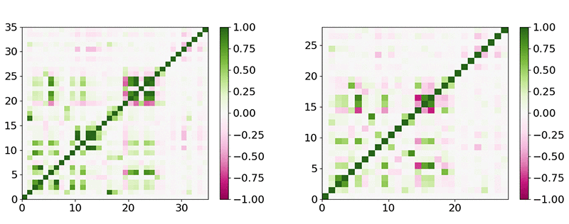
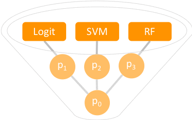


Developing a business strategy by combining machine learning with sensitivity analysis

Machine learning (ML) is routinely used by countless businesses to assist with decision making. In most cases, however, the predictions and business decisions made by ML systems still require the intuition of human users to make judgment calls.

In this post, I show how to combine ML with sensitivity analysis to develop a data-driven business strategy. This post focuses on customer churn (that is, the defection of customers to competitors), while covering problems that often arise when using ML-based analysis. These problems include difficulties with handling incomplete and unbalanced data, deriving strategic options, and quantitatively evaluating the potential impact of those options.

Specifically, I use ML to identify customers who are likely to churn and then use feature importance combined with scenario analysis to derive quantitative and qualitative recommendations. The results can then be used by an organization to make proper strategic and tactical decisions to reduce future churn. This use case illustrates several common issues that arise in the practice of data science, such as:

  • A low signal-to-noise ratio and a lack of clear correlation between features and churn rates
  • Highly imbalanced datasets (wherein 90% of customers in the dataset do not churn)
  • Using probabilistic prediction and adjustment to identify a decision-making mechanism that minimizes the risk of over-investing in churn issues

End-to-end implementation code is available in Amazon SageMaker and as a standalone on Amazon EC2.

In this use case, I consider a fictional company that provides different types of products. I will  call its two key offerings products A and B. I only have partial information about the company’s products and customers. The company has recently seen an increase in customer defection to competitors, also known as churn. The dataset contains information on the diverse attributes of thousands of customers, collected and sorted over several months. Some of these customers have churned, and some have not. Using the list of specific customers, I will predict the probability that any one individual will churn. During this process, I attempt to answer several questions: Can we create a reliable predictive model of customer churn? What variables might explain a customer’s likelihood of churning? What strategies can the company implement to decrease churn?

This post will address the following steps for using ML models to create churn reduction strategies:

Exploring data and engineering new features

I first cover how to explore customer data by looking at simple correlations and associations between individual input features and the churn label. I also examine the associations (called cross-correlations, or covariances) between the features themselves. This allows me to make algorithmic decisions—notably, deciding which features to derive, change, or delete.

Developing an ensemble of ML models

Then, I build several ML algorithms, including automatic feature selection, and combine multiple models to improve performance.

Evaluating and refining ML model performance

In the third section, I test the performance of the different models I have developed. From there, I identify a decision-making mechanism that minimizes the risk of overestimating the number of customers who will churn.

Applying ML models to business strategy design

Finally, in a fourth section, I use the ML results to understand the factors that impact customer churn, derive strategic options, and quantitatively evaluate the impact of those options on churn rates. I do so by performing a sensitivity analysis, where I modify some factors that can be controlled in real life (such as the discount rate) and predict the corresponding reduction in churn expected for different values of this control factor. All predictions will be carried out with the optimal ML model identified in section 3.

Exploring data and engineering new features

Critical issues that often present problems during ML model development include the presence of collinear and low-variance features in the input data, the presence of outliers, and missing data (missing features and missing values for some features). This section describes how to handle each of these issues in Python 3.4 using Amazon SageMaker. (I also evaluated the standalone code on an Amazon EC2 instance with a Deep Learning AMI. Both are available.)

This kind of timestamped data can contain important patterns within certain metrics. I aggregated these metrics into daily, weekly, and monthly segments, which allowed me to develop new features to account for the metrics’ dynamic nature. (See the accompanying notebook for details.)

I then look at simple one-to-one (a.k.a. marginal) correlation and association measures between each individual feature, both original and new. I also look at the correlations between the features and the churn label. (See the following diagrams).

Low-variance features, features that do not change significantly when the churn label changes, can be handled by using marginal correlation and Hamming/Jaccard distances, as depicted in the following table. Hamming/Jaccard distances are measures of similarity designed specifically for binary outcomes. These measures provide perspective on the degree to which each feature might be indicative of churn.

It’s good practice to remove low-variance features as they tend not to change significantly no matter what you’re trying to predict. Consequently, their presence is unlikely to help your analysis and can actually make the learning process less efficient.

The following table shows the top correlations and binary dissimilarities between features and churn. Only the top features are shown out of 48 original and derived features. The Filtered column contains the results that I obtained when I filtered the data for outliers and missing values.

     Pearson correlations with churn
Feature Original Filtered
Margins 0.06 0.1
Forecasted product A 0.03 0.04
Prices 0.03 0.04
$value of discount 0.01 0.01
Current subscription 0.01 0.03
Forecasted product B 0.01 0.01
Number of products -0.02 -0.02
Customer loyalty -0.07 -0.07
     Binary dissimilarities with churn
Feature Hamming Jaccard
Sales channel 1 0.15 0.97
Sales channel 2 0.21 0.96
Sales channel 3 0.45 0.89

The key takeaways from the preceding table are that three sales channels seem inversely correlated to churn and that most marginal correlations with churn are very small (≤ 0.1). Applying filters for outliers and missing values leads to marginal correlations with improved statistical significance. The right column of the preceding table depicts this effect.

The issue of collinear features can be addressed by computing the covariance matrix between all features, as shown in the following diagram. This matrix provides new perspective on the amount of redundancy some features might have. It’s a good practice to remove redundant features because they create biases and demand more computation, again making the learning process less efficient.

The left graph in the preceding diagram indicates that some features, such as prices and some forecasted metrics, are collinear, with ρ > 0.95. I kept only one of each when I designed the ML models that I describe in the next section, which left me with about 40 features, as the right graph in the preceding diagram shows.

The issues of missing and outlier data are often handled by instituting empirical rules, such as deleting observations (customers) when some of their recorded data values are missing, or when they exceed three times the standard deviation across the sample.

Because missing data is a frequent concern, you can impute a missing value with the mean or median across the sample or population as an alternative to deleting observations. That’s what I did here: I replaced missing values with the median for each feature—except for features where more than 40% of data was missing, in which case I deleted the entire feature. The reader should note that a more advanced, best practice approach to imputing missing data is to train a supervised learning model to impute based on other features, but this can require a very large amount of effort so I do not cover it here. When I encountered outliers in the data, I deleted the customers with values beyond six standard deviations from the mean. In total, I deleted 140 out of 16096 (< 1%) observations.

Developing an ensemble of ML models

In this section, I develop and combine multiple ML models to harness the power of multiple ML algorithms. Ensemble modeling also makes it possible to use information from the entire dataset, even though the distribution of the churn label is highly unbalanced, as shown in the following flowchart.

Predicted probability

p0 = (p1 + p2 + p3) / 3

As it’s good practice to remove low-variance features, I further restricted the feature space to the most important features by applying a quick and simple variance filter. This filter removes features that display no variance for more than 95% of customers. To filter features based on their combined effects on customer churn, as opposed to their marginal effects, I carried out an ML-based feature selection using a grid search with stepwise regression. See details in the next section.

Before implementing the ML models, I randomly split the data into two groups, holding out a 30% test set. As discussed in the next section, I also used a 10-fold cross-validation on top of the 70%/30% split. K-folding is an iterative cycle that averages the performance over K evaluations, each testing on a separate K% holdout set of the data.

Three ML algorithms—logistic regression, support vector machine, and random forest—were trained separately, then combined in an ensemble, as depicted in the preceding flowchart. The ensemble approach is referred to as soft-voting in the literature because it takes the average probability of the different models and uses it to classify customer churn (also visible in the preceding flowchart).

Customers with churn represent only 10% of the data; therefore, the dataset is unbalanced. I tested two approaches to deal with class imbalance.

  • In the first, simplest approach, the training is based on a random sampling of the abundant class (customers who didn’t churn) to match the size of the rare class (customers who did).
  • In the second approach (shown in the following chart), I based the training on an ensemble of nine models using nine random samples of the abundant class (without replacement) and a full sample of the rare class for each model. I chose a 9-fold because the class imbalance is approximately 1-to-9 (as shown in the histogram in the following diagram). Therefore, 1-9 is the amount of sampling required to use all or nearly all of the data in the abundant class. This approach is more complex, but it uses all available information, improving generalization. I evaluate its effectiveness in the following section.

For both approaches, the performance is evaluated on a test set wherein class imbalance is maintained to account for real-world circumstances.

Evaluating and refining ML model performance

In this section, I test the performance of the different models I developed in the previous section. I then identify a decision-making mechanism that minimizes the risk of overestimating the number of customers who might churn (called the false positive rate).

The so-called receiver-operator characteristic (ROC) curve is often used in ML performance evaluation to complement contingency tables. The ROC curve provides an invariant measure of accuracy when changing the probability threshold to infer positive and negative classes (in this project, churn and no churn, respectively). It involves plotting all accurate positive predictions (true positives) against false positives, also known as fall out. See the following table.

The probabilities predicted by the different ML models are by default calibrated so that values where p > 0.5 correspond to one class and values where p < 0.5 correspond to the other class. This threshold is a hyperparameter that can be fine-tuned to minimize misclassified instances of one class. This is at the expense of increasing misclassification in the other, which can affect the accuracy and precision of different performance measures. In contrast, the area under the ROC curve is an invariant measure of performance—it remains the same for any threshold.

The following table depicts the performance of different ML models with a random sampling of the rare class (baseline) and the 9-fold ensemble of learners. You can see that the random forest has the best performance, and further that the 9-fold ensemble is better at generalizing, with an ROC AUC score of 0.68. This model is the best performer.

     Performance measures
Algorithm Accuracy Brier ROC
Logit 56% 0.24 0.64
Stepwise 56% 0.24 0.64
SVM 57% 0.24 0.63
RF 65% 0.24 0.67
Ensemble 61% 0.23 0.66
9-Logit Ensemble 55% 0.26 0.64
9-SVM Ensemble 61% 0.25 0.63
9-RF Ensemble 70% 0.24 0.68
9-Ensemble Ensemble 61% 0.25 0.65

The following chart depicts the performance of the overall best learner (the 9-fold ensemble of random forest learners) and the optimization for precision and fall out. When using a probability threshold of 0.5, the best performer can predict 69% of the customers who might churn though with significant fall out of 42%.

Looking at the ROC curve, you can see that the same model can predict 30% of customers who will churn, with fall out minimized at 10%. Using a grid search, I found that the threshold is p = 0.56. If you want to minimize the risk of overestimating the number of customers who will churn (for example, because the attempts we make to keep those customers could be expensive), this is the model you might want to use.

Applying ML models to business strategy design

In this section, I use the ML models that I have developed to better understand the factors that impact customer churn, to derive strategic options for decreasing churn, and to evaluate the quantitative impact that deploying those options might have on churn rates.

I used a stepwise logistic regression to assess the importance of features while taking into account their combined effect on churn. As shown in the following graph, the regression identifies 12 key features. The prediction score is highest when I include these 12 features in the regression model.

Among these 12 factors, the net margin, the forecasted purchase of products A and B, and the index that indicates multiple-product customers are the features that have the greatest tendency to induce churn. The factors that tended to reduce churn included three sales channels, one marketing campaign, the value of the discount, overall subscriptions, the loyalty of the customer, and the overall number of products purchased.

Therefore, providing a discount to customers with the highest propensity to churn seems to be a simple and effective strategy. Other strategic levers have also been identified, including boosting synergy between products other than A and B, sales channels 1–3, the marketing campaign, and long-term contracts. According to the data, pulling these levers is likely to decrease customer churn.

Finally, I used a sensitivity analysis: I applied a discount of up to 40% to customers that the ML model identified as likely to churn, then re-ran the model to evaluate how many customers were still predicted to churn after incorporating the discount.

When I set the model at a p threshold of 0.6 to minimize fall out to 10%, my analysis predicts that a 20% discount reduces churn by 25%. Given that the true positive rate at this threshold is about 30%, this analysis indicates that a 20% discount approach could eliminate at least 8% of churn. See the following graph for details. The discount strategy is a simple first step that an organization experiencing customer churn might consider taking to mitigate the issue.

Conclusion

In this post, I demonstrated how to do the following:

  • Explore data and derive new features in order to minimize issues stemming from missing data and a low signal-to-noise ratio.
  • Design an ensemble of ML models to handle strongly unbalanced datasets.
  • Select the best-performing models and refine the decision threshold to maximize precision and minimize fall out.
  • Use the results to derive strategic options and quantitatively assess their impact on churn rates.

In this particular use case, I developed a model that can identify 30% of customers who are likely to churn while limiting fall out to 10%. This study supports the efficacy of deploying a short-term tactic of offering discounts and instituting a long-term strategy based on building synergy between services and sales channels to retain more customers.

If you would like to run the code that produce the data and insights described in this blog post, just download the notebook and associated data file, then run each each cell one at a time.


About the author

Jeremy David Curuksu is a data scientist and consultant in AI-ML at the Amazon Machine Learning Solutions Lab (AWS). He holds a MSc and a PhD in applied mathematics, and was a research scientist at EPFL (Switzerland) and MIT (US). He is the author of multiple scientific peer-reviewed articles and the book Data Driven which introduces management consulting in the new age of data science.