Posted by Andrew Helton, Editor, Google Research Communications
This week, Vancouver hosts the 33rd annual Conference on Neural Information Processing Systems (NeurIPS 2019), the biggest machine learning conference of the year. The conference includes invited talks, demonstrations and presentations of some of the latest in machine learning research. As a Diamond Sponsor of NeurIPS 2019, Google will have a strong presence at NeurIPS 2019 with more than 500 Googlers attending in order to contribute to, and learn from, the broader academic research community via talks, posters, workshops, competitions and tutorials. We will be presenting work that pushes the boundaries of what is possible in language understanding, translation, speech recognition and visual & audio perception, with Googlers co-authoring more than 130 accepted papers.
If you are attending NeurIPS 2019, we hope you’ll stop by our booth and chat with our researchers about the projects and opportunities at Google that go into solving the world’s most challenging research problems, and to see demonstrations of some of the exciting research we pursue, such as ML-based Flood Forecasting, AI for Social Good, Google Research Football, Google Dataset Search, TF-Agents and much more. You can also learn more about our work being presented in the list below (Google affiliations highlighted in blue).
NeurIPS Foundation Board
Samy Bengio, Corinna Cortes
NeurIPS Advisory Board
John C. Platt, Fernando Pereira, Dale Schuurmans
NeurIPS Program Committee
Program Chair: Hugo Larochelle
Diversity & Inclusion Co-Chair: Katherine Heller
Meetup Chair: Nicolas La Roux
Party Co-Chair: Pablo Samuel Castro
Senior Area Chairs include: Amir Globerson, Claudio Gentile, Cordelia Schmid, Corinna Cortes, Dale Schuurmans, Elad Hazan, Honglak Lee, Mehryar Mohri, Peter Bartlett, Satyen Kale, Sergey Levine, Surya Ganguli
Area Chairs include: Afshin Rostamizadeh, Alex Kulesza, Amin Karbasi, Andrew Dai, Been Kim, Boqing Gong, Brainslav Kveton, Ce Liu, Charles Sutton, Chelsea Finn, Cho-Jui Hsieh, D Sculley, Danny Tarlow, David Held, Denny Zhou, Yann Dauphin, Dustin Tran, Hartmut Neven, Hossein Mobahi, Ilya Tolstikhin, Jasper Snoek, Jean-Philippe Vert, Jeffrey Pennington, Kevin Swersky, Kun Zhang, Kunal Talwar, Lihong Li, Manzil Zaheer, Marc G Bellemare, Marco Cuturi, Maya Gupta, Meg Mitchell, Minmin Chen, Mohammad Norouzi, Moustapha Cisse, Olivier Bachem, Qiang Liu, Rong Ge, Sanjiv Kumar, Sanmi Koyejo, Sebastian Nowozin, Sergei Vassilvitskii, Shivani Agarwal, Slav Petrov, Srinadh Bhojanapalli, Stephen Bach, Timnit Gebru, Tomer Koren, Vitaly Feldman, William Cohen, Yann Dauphin, Nicolas La Roux
NeurIPS Workshops Program Committee
Yann Dauphin, Honglak Lee, Sebastian Nowozin, Fernanda Viegas
NeurIPS Invited Talk
Social Intelligence
Blaise Aguera y Arcas
Accepted Papers
Memory Efficient Adaptive Optimization
Rohan Anil, Vineet Gupta, Tomer Koren, Yoram Singer
Stand-Alone Self-Attention in Vision Models
Niki Parmar, Prajit Ramachandran, Ashish Vaswani, Irwan Bello, Anselm Levskaya, Jon Shlens
High Fidelity Video Prediction with Large Neural Nets
Ruben Villegas, Arkanath Pathak, Harini Kannan, Dumitru Erhan, Quoc V. Le, Honglak Lee
Unsupervised Learning of Object Structure and Dynamics from Videos
Matthias Minderer, Chen Sun, Ruben Villegas, Forrester Cole, Kevin Murphy, Honglak Lee
GPipe: Efficient Training of Giant Neural Networks using Pipeline Parallelism
Yanping Huang, Youlong Cheng, Ankur Bapna, Orhan Firat, Dehao Chen, Mia Chen, Hyouk Joong Lee, Jiquan Ngiam, Quoc V. Le, Yonghui Wu, Zhifeng Chen
Quadratic Video Interpolation
Xiangyu Xu, Li Si-Yao, Wenxiu Sun, Qian Yin, Ming-Hsuan Yang
Online Stochastic Shortest Path with Bandit Feedback and Unknown Transition Function
Aviv Rosenberg, Yishay Mansour
Individual Regret in Cooperative Nonstochastic Multi-Armed Bandits
Yogev Bar-On, Yishay Mansour
Learning to Screen
Alon Cohen, Avinatan Hassidim, Haim Kaplan, Yishay Mansour, Shay Moran
DualDICE: Behavior-Agnostic Estimation of Discounted Stationary Distribution Corrections
Ofir Nachum, Yinlam Chow, Bo Dai, Lihong Li
A Kernel Loss for Solving the Bellman Equation
Yihao Feng, Lihong Li, Qiang Liu
Accurate Uncertainty Estimation and Decomposition in Ensemble Learning
Jeremiah Liu, John Paisley, Marithani-Anna Kioumourtzoglou, Brent Coull
Saccader: Improving Accuracy of Hard Attention Models for Vision
Gamaleldin F. Elsayed, Simon Kornblith, Quoc V. Le
Invertible Convolutional Flow
Mahdi Karami, Dale Schuurmans, Jascha Sohl-Dickstein, Laurent Dinh, Daniel Duckworth
Hypothesis Set Stability and Generalization
Dylan J. Foster, Spencer Greenberg, Satyen Kale, Haipeng Luo, Mehryar Mohri, Karthik Sridharan
Bandits with Feedback Graphs and Switching Costs
Raman Arora, Teodor V. Marinov, Mehryar Mohri
Regularized Gradient Boosting
Corinna Cortes, Mehryar Mohri, Dmitry Storcheus
Logarithmic Regret for Online Control
Naman Agarwal, Elad Hazan, Karan Singh
Sampled Softmax with Random Fourier Features
Ankit Singh Rawat, Jiecao Chen, Felix Yu, Ananda Theertha Suresh, Sanjiv Kumar
Multilabel Reductions: What is My Loss Optimising?
Aditya Krishna Menon, Ankit Singh Rawat, Sashank Reddi, Sanjiv Kumar
MetaInit: Initializing Learning by Learning to Initialize
Yann N. Dauphin, Sam Schoenholz
Generalization Bounds for Neural Networks via Approximate Description Length
Amit Daniely, Elad Granot
Variance Reduction of Bipartite Experiments through Correlation Clustering
Jean Pouget-Abadie, Kevin Aydin, Warren Schudy, Kay Brodersen, Vahab Mirrokni
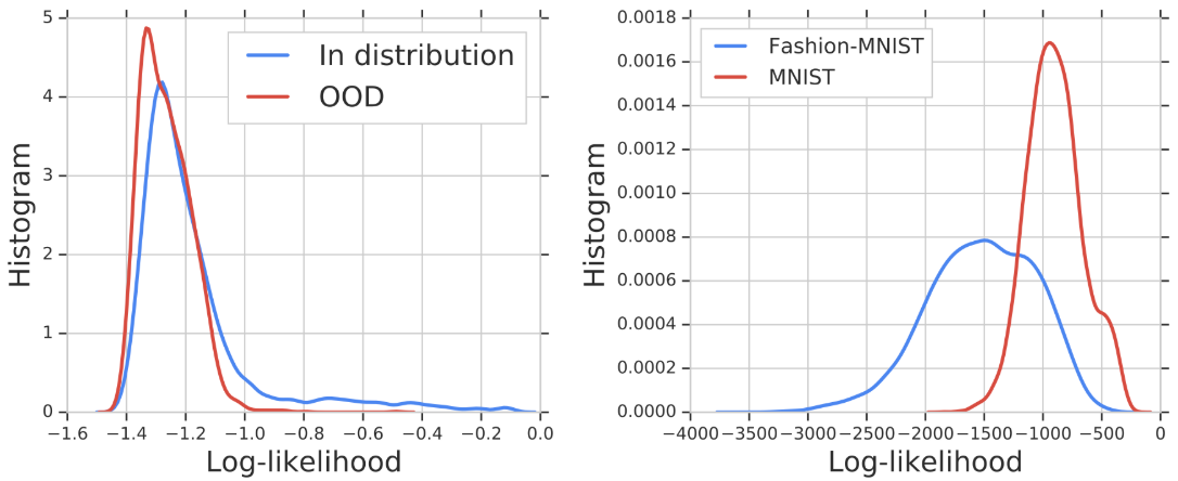
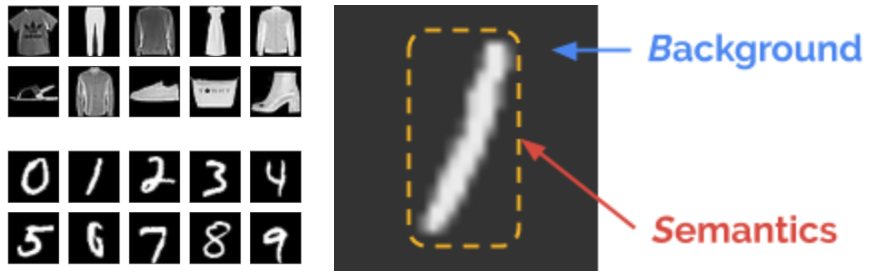
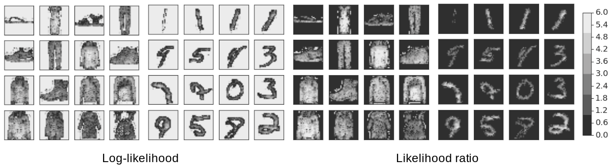
Likelihood Ratios for Out-of-Distribution Detection
Jie Ren, Peter J. Liu, Emily Fertig, Jasper Snoek, Ryan Poplin, Mark A. DePristo, Joshua V. Dillon, Balaji Lakshminarayanan
Can You Trust Your Model’s Uncertainty? Evaluating Predictive Uncertainty Under Dataset Shift
Yaniv Ovadia, Emily Fertig, Jie Jessie Ren, D. Sculley, Josh Dillon, Sebastian Nowozin, Zack Nado, Balaji Lakshminarayanan, Jasper Snoek
Surrogate Objectives for Batch Policy Optimization in One-step Decision Making
Minmin Chen, Ramki Gummadi, Chris Harris, Dale Schuurmans
Globally Optimal Learning for Structured Elliptical Losses
Yoav Wald, Nofar Noy, Gal Elidan, Ami Wiesel
DPPNet: Approximating Determinantal Point Processes with Deep Networks
Zelda Mariet, Yaniv Ovadia, Jasper Snoek
Graph Normalizing Flows
Jenny Liu, Aviral Kumar, Jimmy Ba, Jamie Kiros, Kevin Swersky
When Does Label Smoothing Help?
Rafael Muller, Simon Kornblith, Geoff Hinton
On the Role of Inductive Bias From Simulation and the Transfer to the Real World: a new Disentanglement Dataset
Muhammad Waleed Gondal, Manuel Wüthrich, Đorđe Miladinović, Francesco Locatello, Martin Breidt, Valentin Volchkov, Joel Akpo, Olivier Bachem, Bernhard Schölkopf, Stefan Bauer
On the Fairness of Disentangled Representations
Francesco Locatello, Gabriele Abbati, Tom Rainforth, Stefan Bauer, Bernhard Schölkopf, Olivier Bachem
Are Disentangled Representations Helpful for Abstract Visual Reasoning?
Sjoerd van Steenkiste, Francesco Locatello, Jürgen Schmidhuber, Olivier Bachem
Don’t Blame the ELBO! A Linear VAE Perspective on Posterior Collapse
James Lucas, George Tucker, Roger Grosse, Mohammad Norouzi
Stabilizing Off-Policy Q-Learning via Bootstrapping Error Reduction
Aviral Kumar, Justin Fu, Matthew Soh, George Tucker, Sergey Levine
Optimizing Generalized Rate Metrics with Game Equilibrium
Harikrishna Narasimhan, Andrew Cotter, Maya Gupta
On Making Stochastic Classifiers Deterministic
Andrew Cotter, Harikrishna Narasimhan, Maya Gupta
Discrete Flows: Invertible Generative Models of Discrete Data
Dustin Tran, Keyon Vafa, Kumar Agrawal, Laurent Dinh, Ben Poole
Graph Agreement Models for Semi-Supervised Learning
Otilia Stretcu, Krishnamurthy Viswanathan, Dana Movshovitz-Attias, Emmanouil Platanios, Andrew Tomkins, Sujith Ravi
A Robust Non-Clairvoyant Dynamic Mechanism for Contextual Auctions
Yuan Deng, Sébastien Lahaie, Vahab Mirrokni
Adversarial Robustness through Local Linearization
Chongli Qin, James Martens, Sven Gowal, Dilip Krishnan, Krishnamurthy (Dj) Dvijotham, Alhusein Fawzi, Soham De, Robert Stanforth, Pushmeet Kohli
A Geometric Perspective on Optimal Representations for Reinforcement Learning
Marc G. Bellemare, Will Dabney, Robert Dadashi, Adrien Ali Taiga, Pablo Samuel Castro, Nicolas Le Roux, Dale Schuurmans, Tor Lattimore, Clare Lyle
Online Learning via the Differential Privacy Lens
Jacob Abernethy, Young Hun Jung, Chansoo Lee, Audra McMillan, Ambuj Tewari
Reducing the Variance in Online Optimization by Transporting Past Gradients
Sébastien M. R. Arnold, Pierre-Antoine Manzagol, Reza Babanezhad, Ioannis Mitliagkas, Nicolas Le Roux
Universality and Individuality in Neural Dynamics Across Large Populations of Recurrent Networks
Niru Maheswaranathan, Alex Williams, Matt Golub, Surya Ganguli, David Sussillo
Reverse Engineering Recurrent Networks for Sentiment Classification Reveals Line Attractor Dynamics
Niru Maheswaranathan, Alex H. Williams, Matthew D. Golub, Surya Ganguli, David Sussillo
Strategizing Against No-Regret Learners
Yuan Deng, Jon Schneider, Balasubramanian Sivan
Prior-Free Dynamic Auctions with Low Regret Buyers
Yuan Deng, Jon Schneider, Balasubramanian Sivan
Private Stochastic Convex Optimization with Optimal Rates
Raef Bassily, Vitaly Feldman, Kunal Talwar, Abhradeep Thakurta
Computational Separations between Sampling and Optimization
Kunal Talwar
Momentum-Based Variance Reduction in Non-Convex SGD
Ashok Cutkosky and Francesco Orabona
Kernel Truncated Randomized Ridge Regression: Optimal Rates and Low Noise Acceleration
Kwang-Sung Jun, Ashok Cutkosky, Francesco Orabona
Fast and Flexible Multi-Task Classification using Conditional Neural Adaptive Processes
James Requeima, Jonathan Gordon, John Bronskill, Sebastian Nowozin, Richard E. Turner
Icebreaker: Element-wise Active Information Acquisition with Bayesian Deep Latent Gaussian Model
Wenbo Gong, Sebastian Tschiatschek, Richard E. Turner, Sebastian Nowozin, Jose Miguel Hernandez-Lobato, Cheng Zhang
Multiview Aggregation for Learning Category-Specific Shape Reconstruction
Srinath Sridhar, Davis Rempe, Julien Valentin, Sofien Bouaziz, Leonidas J. Guibas
Visualizing and Measuring the Geometry of BERT
Andy Coenen, Emily Reif, Ann Yuan, Been Kim, Adam Pearce, Fernanda Viégas, Martin Wattenberg
Locality-Sensitive Hashing for f-Divergences: Mutual Information Loss and Beyond
Lin Chen, Hossein Esfandiari, Thomas Fu, Vahab S. Mirrokni
A Benchmark for Interpretability Methods in Deep Neural Networks
Sara Hooker, Dumitru Erhan, Pieter-jan Kindermans, Been Kim
Practical and Consistent Estimation of f-Divergences
Paul Rubenstein, Olivier Bousquet, Josip Djolonga, Carlos Riquelme, Ilya Tolstikhin
Tree-Sliced Variants of Wasserstein Distances
Tam Le, Makoto Yamada, Kenji Fukumizu, Marco Cuturi
Game Design for Eliciting Distinguishable Behavior
Fan Yang, Liu Leqi, Yifan Wu, Zachary Lipton, Pradeep Ravikumar, Tom M Mitchell, William Cohen
Differentially Private Anonymized Histograms
Ananda Theertha Suresh
Locally Private Gaussian Estimation
Matthew Joseph, Janardhan Kulkarni, Jieming Mao, Zhiwei Steven Wu
Exponential Family Estimation via Adversarial Dynamics Embedding
Bo Dai, Zhen Liu, Hanjun Dai, Niao He, Arthur Gretton, Le Song, Dale Schuurmans
Learning to Predict Without Looking Ahead: World Models Without Forward Prediction
C. Daniel Freeman, Luke Metz, David Ha
Adaptive Density Estimation for Generative Models
Thomas Lucas, Konstantin Shmelkov, Karteek Alahari, Cordelia Schmid, Jakob Verbeek
Weight Agnostic Neural Networks
Adam Gaier, David Ha
Retrosynthesis Prediction with Conditional Graph Logic Network
Hanjun Dai, Chengtao Li, Connor Coley, Bo Dai, Le Song
Large Scale Structure of Neural Network Loss Landscapes
Stanislav Fort, Stainslaw Jastrzebski
Off-Policy Evaluation via Off-Policy Classification
Alex Irpan, Kanishka Rao, Konstantinos Bousmalis, Chris Harris, Julian Ibarz, Sergey Levine
Domes to Drones: Self-Supervised Active Triangulation for 3D Human Pose Reconstruction
Aleksis Pirinen, Erik Gartner, Cristian Sminchisescu
Energy-Inspired Models: Learning with Sampler-Induced Distributions
Dieterich Lawson, George Tucker, Bo Dai, Rajesh Ranganath
From Deep Learning to Mechanistic Understanding in Neuroscience: The Structure of Retinal Prediction
Hidenori Tanaka, Aran Nayebi, Niru Maheswaranathan, Lane McIntosh, Stephen Baccus, Surya Ganguli
Language as an Abstraction for Hierarchical Deep Reinforcement Learning
Yiding Jiang, Shixiang Gu, Kevin Murphy, Chelsea Finn
Bayesian Layers: A Module for Neural Network Uncertainty
Dustin Tran, Michael W. Dusenberry, Mark van der Wilk, Danijar Hafner
Adaptive Temporal-Difference Learning for Policy Evaluation with Per-State Uncertainty Estimates
Hugo Penedones, Carlos Riquelme, Damien Vincent, Hartmut Maennel, Timothy Mann, Andre Barreto, Sylvain Gelly, Gergely Neu
A Unified Framework for Data Poisoning Attack to Graph-based Semi-Supervised Learning
Xuanqing Liu, Si Si, Xiaojin Zhu, Yang Li, Cho-Jui Hsieh
MixMatch: A Holistic Approach to Semi-Supervised Learning
David Berthelot, Nicholas Carlini, Ian Goodfellow (work done while at Google), Avital Oliver, Nicolas Papernot, Colin Raffel
SMILe: Scalable Meta Inverse Reinforcement Learning through Context-Conditional Policies
Seyed Kamyar Seyed Ghasemipour, Shixiang (Shane) Gu, Richard Zemel
Limits of Private Learning with Access to Public Data
Noga Alon, Raef Bassily, Shay Moran
Regularized Weighted Low Rank Approximation
Frank Ban, David Woodruff, Richard Zhang
Unsupervised Curricula for Visual Meta-Reinforcement Learning
Allan Jabri, Kyle Hsu, Abhishek Gupta, Benjamin Eysenbach, Sergey Levine, Chelsea Finn
Secretary Ranking with Minimal Inversions
Sepehr Assadi, Eric Balkanski, Renato Paes Leme
Mixtape: Breaking the Softmax Bottleneck Efficiently
Zhilin Yang, Thang Luong, Russ Salakhutdinov, Quoc V. Le
Budgeted Reinforcement Learning in Continuous State Space
Nicolas Carrara, Edouard Leurent, Romain Laroche, Tanguy Urvoy, Odalric-Ambrym Maillard, Olivier Pietquin
From Complexity to Simplicity: Adaptive ES-Active Subspaces for Blackbox Optimization
Krzysztof Choromanski, Aldo Pacchiano, Jack Parker-Holder, Yunhao Tang
Generalization Bounds for Neural Networks via Approximate Description Length
Amit Daniely, Elad Granot
Flattening a Hierarchical Clustering through Active Learning
Fabio Vitale, Anand Rajagopalan, Claudio Gentile
Robust Attribution Regularization
Jiefeng Chen, Xi Wu, Vaibhav Rastogi, Yingyu Liang, Somesh Jha
Robustness Verification of Tree-based Models
Hongge Chen, Huan Zhang, Si Si, Yang Li, Duane Boning, Cho-Jui Hsieh
Meta Architecture Search
Albert Shaw, Wei Wei, Weiyang Liu, Le Song, Bo Dai
Contextual Bandits with Cross-Learning
Santiago Balseiro, Negin Golrezaei, Mohammad Mahdian, Vahab Mirrokni, Jon Schneider
Dynamic Incentive-Aware Learning: Robust Pricing in Contextual Auctions
Negin Golrezaei, Adel Javanmard, Vahab Mirrokni
Optimizing Generalized Rate Metrics with Three Players
Harikrishna Narasimhan, Andrew Cotter, Maya Gupta
Noise-Tolerant Fair Classification
Alexandre Louis Lamy, Ziyuan Zhong, Aditya Krishna Menon, Nakul Verma
Towards Automatic Concept-based Explanations
Amirata Ghorbani, James Wexler, James Zou, Been Kim
Locally Private Learning without Interaction Requires Separation
Amit Daniely, Vitaly Feldman
Learning GANs and Ensembles Using Discrepancy
Ben Adlam, Corinna Cortes, Mehryar Mohri, Ningshan Zhang
CondConv: Conditionally Parameterized Convolutions for Efficient Inference
Brandon Yang, Gabriel Bender, Quoc V. Le, Jiquan Ngiam
A Fourier Perspective on Model Robustness in Computer Vision
Dong Yin, Raphael Gontijo Lopes, Jonathon Shlens, Ekin D. Cubuk, Justin Gilmer
Robust Bi-Tempered Logistic Loss Based on Bregman Divergences
Ehsan Amid, Manfred K. Warmuth, Rohan Anil, Tomer Koren
When Does Label Smoothing Help?
Rafael Müller, Simon Kornblith, Geoffrey Hinton
Memory Efficient Adaptive Optimization
Rohan Anil, Vineet Gupta, Tomer Koren, Yoram Singer
Which Algorithmic Choices Matter at Which Batch Sizes? Insights From a Noisy Quadratic Model
Guodong Zhang, Lala Li, Zachary Nado, James Martens, Sushant Sachdeva, George E. Dahl, Christopher J. Shallue, Roger Grosse
Wide Neural Networks of Any Depth Evolve as Linear Models Under Gradient Descent
Jaehoon Lee, Lechao Xiao, Samuel S. Schoenholz, Yasaman Bahri, Roman Novak, Jascha Sohl-Dickstein, Jeffrey Pennington
Universality and Individuality in Neural Dynamics Across Large Populations of Recurrent Networks
Niru Maheswaranathan, Alex H. Williams, Matthew D. Golub, Surya Ganguli, David Sussillo
Abstract Reasoning with Distracting Features
Kecheng Zheng, Zheng-Jun Zha, Wei Wei
Search on the Replay Buffer: Bridging Planning and Reinforcement Learning
Benjamin Eysenbach, Ruslan Salakhutdinov, Sergey Levine
Differentiable Ranking and Sorting Using Optimal Transport
Marco Cuturi, Olivier Teboul, Jean-Philippe Vert
XLNet: Generalized Autoregressive Pretraining for Language Understanding
Zhilin Yang, Zihang Dai, Yiming Yang, Jaime Carbonell, Ruslan Salakhutdinov, Quoc V. Le
Private Learning Implies Online Learning: An Efficient Reduction
Alon Gonen, Elad Hazan, Shay Moran
Evaluating Protein Transfer Learning with TAPE
Roshan Rao, Nicholas Bhattacharya, Neil Thomas, Yan Duan, Peter Chen, John Canny, Pieter Abbeel, Yun Song
Tight Dimensionality Reduction for Sketching Low Degree Polynomial Kernels
Michela Meister, Tamas Sarlos, David P. Woodruff
No Pressure! Addressing the Problem of Local Minima in Manifold Learning Algorithms
Max Vladymyrov
Subspace Detours: Building Transport Plans that are Optimal on Subspace Projections
Boris Muzellec, Marco Cuturi
Online Stochastic Shortest Path with Bandit Feedback and Unknown Transition Function
Aviv Rosenberg, Yishay Mansour
Private Learning Implies Online Learning: An Efficient Reduction
Alon Gonen, Elad Hazan, Shay Moran
On the Fairness of Disentangled Representations
Francesco Locatello, Gabriele Abbati, Tom Rainforth, Stefan Bauer, Bernhard Schölkopf, Olivier Bachem
On the Transfer of Inductive Bias from Simulation to the Real World: a New Disentanglement Dataset
Muhammad Waleed Gondal, Manuel Wüthrich, Ðorde Miladinovíc, Francesco Locatello, Martin Breidt, Valentin Volchkov, Joel Akpo, Olivier Bachem, Bernhard Schölkopf, Stefan Bauer
Stacked Capsule Autoencoders
Adam R. Kosiorek, Sara Sabour, Yee Whye Teh, Geoffrey E. Hinton
Wasserstein Dependency Measure for Representation Learning
Sherjil Ozair, Corey Lynch, Yoshua Bengio, Aaron van den Oord, Sergey Levine, Pierre Sermanet
Sampling Sketches for Concave Sublinear Functions of Frequencies
Edith Cohen, Ofir Geri
Hamiltonian Neural Networks
Sam Greydanus, Misko Dzamba, Jason Yosinski
Evaluating Protein Transfer Learning with TAPE
Roshan Rao, Nicholas Bhattacharya, Neil Thomas, Yan Duan, Xi Chen, John Canny, Pieter Abbeel, Yun S. Song
Computational Mirrors: Blind Inverse Light Transport by Deep Matrix Factorization
Miika Aittala, Prafull Sharma, Lukas Murmann, Adam B. Yedidia, Gregory W. Wornell, William T. Freeman, Frédo Durand
Quadratic Video Interpolation
Xiangyu Xu, Li Siyao, Wenxiu Sun, Qian Yin, Ming-Hsuan Yang
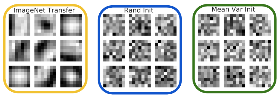
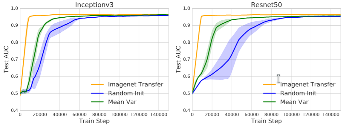
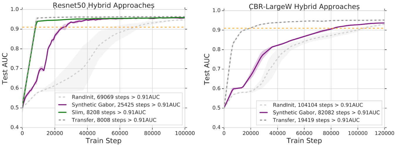
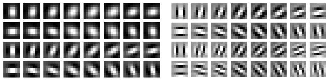
Transfusion: Understanding Transfer Learning for Medical Imagings
Maithra Raghu, Chiyuan Zhang, Jon Kleinberg, Samy Bengio
XLNet: Generalized Autoregressive Pretraining for Language Understanding
Zhilin Yang, Zihang Dai, Yiming Yang, Jaime Carbonell, Ruslan Salakhutdinov, Quoc V. Le
Differentially Private Covariance Estimation
Kareem Amin, Travis Dick, Alex Kulesza, Andres Munoz, Sergei Vassilvitskii
Private Stochastic Convex Optimization with Optimal Rates
Raef Bassily, Vitaly Feldman, Kunal Talwar, Abhradeep Thakurta
Learning Transferable Graph Exploration
Hanjun Dai, Yujia Li, Chenglong Wang, Rishabh Singh, Po-Sen Huang, Pushmeet Kohli
Neural Attribution for Semantic Bug-Localization in Student Programs
Rahul Gupta, Aditya Kanade, Shirish Shevade
PyTorch: An Imperative Style, High-Performance Deep Learning Library
Adam Paszke, Sam Gross, Francisco Massa, Adam Lerer, James Bradbury, Gregory Chanan, Trevor Killeen, Zeming Lin, Natalia Gimelshein, Luca Antiga, Alban Desmaison, Andreas Kopf, Edward Yang, Zachary DeVito, Martin Raison, Alykhan Tejani, Sasank Chilamkurthy, Benoit Steiner, Lu Fang, Junjie Bai, Soumith Chintala
Breaking the Glass Ceiling for Embedding-Based Classifiers for Large Output Spaces
Chuan Guo, Ali Mousavi, Xiang Wu, Daniel Holtmann-Rice, Satyen Kale, Sashank Reddi, Sanjiv Kumar
Efficient Rematerialization for Deep Networks
Ravi Kumar, Manish Purohit, Zoya Svitkina, Erik Vee, Joshua R. Wang
Momentum-Based Variance Reduction in Non-Convex SGD
Ashok Cutkosky, Francesco Orabona
Kernel Truncated Randomized Ridge Regression: Optimal Rates and Low Noise Acceleration
Kwang-Sung Jun, Ashok Cutkosky, Francesco Orabona
Workshops
3rd Conversational AI: Today’s Practice and Tomorrow’s Potential
Organizers include: Bill Byrne
AI for Humanitarian Assistance and Disaster Response Workshop
Invited Speakers include: Yossi Matias
Bayesian Deep Learning
Organizers include: Kevin P Murphy
Beyond First Order Methods in Machine Learning Systems
Invited Speakers include: Elad Hazan
Biological and Artificial Reinforcement Learning
Invited Speakers include: Igor Mordatch
Context and Compositionality in Biological and Artificial Neural Systems
Invited Speakers include: Kenton Lee
Deep Reinforcement Learning
Organizers include: Chelsea Finn
Document Intelligence
Organizers include: Tania Bedrax Weiss
Federated Learning for Data Privacy and Confidentiality
Organizers include: Jakub Konečný, Brendan McMahan
Invited Speakers include: Françoise Beaufays, Daniel Ramage
Graph Representation Learning
Organizers include: Rianne van den Berg
Human-Centric Machine Learning
Invited Speakers include: Been Kim
Information Theory and Machine Learning
Organizers include: Ben Poole
Invited Speakers include: Alex Alemi
KR2ML – Knowledge Representation and Reasoning Meets Machine Learning
Invited Speakers include: William Cohen
Learning Meaningful Representations of Life
Organizers include: Jasper Snoek, Alexander Wiltschko
Learning Transferable Skills
Invited Speakers include: David Ha
Machine Learning for Creativity and Design
Organizers include: Adam Roberts, Jesse Engel
Machine Learning for Health (ML4H): What Makes Machine Learning in Medicine Different?
Invited Speakers include: Lily Peng, Alan Karthikesalingam, Dale Webster
Machine Learning and the Physical Sciences
Speakers include: Yasaman Bahri, Samual Schoenholz
ML for Systems
Organizers include: Milad Hashemi, Kevin Swersky, Azalia Mirhoseini, Anna Goldie
Invited Speakers include: Jeff Dean
Optimal Transport for Machine Learning
Organizers include: Marco Cuturi
The Optimization Foundations of Reinforcement Learning
Organizers include: Bo Dai, Nicolas Le Roux, Lihong Li, Dale Schuurmans
Privacy in Machine Learning
Invited Speakers include: Brendan McMahan
Program Transformations for ML
Organizers include: Pascal Lamblin, Alexander Wiltschko, Bart van Merrienboer, Emily Fertig
Invited Speakers include: Skye Wanderman-Milne
Real Neurons & Hidden Units: Future Directions at the Intersection of Neuroscience and Artificial Intelligence
Organizers include: David Sussillo
Robot Learning: Control and Interaction in the Real World
Organizers include: Stefan Schaal
Safety and Robustness in Decision Making
Organizers include: Yinlam Chow
Science Meets Engineering of Deep Learning
Invited Speakers include: Yasaman Bahri, Surya Ganguli, Been Kim, Surya Ganguli
Sets and Partitions
Organizers include: Manzil Zaheer, Andrew McCallum
Invited Speakers include: Amr Ahmed
Tackling Climate Change with ML
Organizers include: John Platt
Invited Speakers include: Jeff Dean
Visually Grounded Interaction and Language
Invited Speakers include: Jason Baldridge
Workshop on Machine Learning with Guarantees
Invited Speakers include: Mehryar Mohri
Tutorials
Representation Learning and Fairness
Organizers include: Moustapha Cisse, Sanmi Koyejo