Improving Out-of-Distribution Detection in Machine Learning Models
Successful deployment of machine learning systems requires that the system be able to distinguish between data that is anomalous or significantly different from that used in training. This is particularly important for deep neural network classifiers, which might classify such out-of-distribution (OOD) inputs into in-distribution classes with high confidence. This is critically important when these predictions inform real-world decisions.
For example, one challenging application of machine learning models to real-world applications is bacteria identification based on genomic sequences. Bacteria detection is crucial for diagnosis and treatment of infectious diseases, such as sepsis, and for identifying foodborne pathogens. New bacterial classes continue to be discovered over the years, and while a neural network classifier trained on the known classes achieves high accuracy as measured through cross-validation, deploying a model is challenging, since real-world data is ever evolving and will inevitably contain genomes from unseen classes (OOD inputs) not present in the training data.
 |
| New bacterial classes are gradually discovered over the years. A classifier trained on known classes achieves high accuracy for test inputs belonging to known classes, but can wrongly classify inputs from unknown classes (i.e., out-of-distribution) into known classes with high confidence. |
In “Likelihood Ratios for Out-of-Distribution Detection”, presented at NeurIPS 2019, we proposed and released a realistic benchmark dataset of genomic sequences for OOD detection that is inspired by the real-world challenges described above. We tested existing methods for OOD detection using generative models on genomic sequences and found that the likelihood values — i.e., the model’s probability that an input comes from the distribution as estimated using in-distribution data — was often in error. This phenomenon has also been observed in recent work on deep generative models of images. We explain this phenomenon through the effect of background statistics and propose a likelihood-ratio based solution that significantly improves the accuracy of OOD detection.
Why Do Density Models Fail At OOD Detection?
To mimic the real problem and systematically evaluate different methods, we built a new bacterial dataset using data sourced from the publicly available NCBI catalog of prokaryotic genome sequences. To mimic sequencing data, we fragmented genomes into short sequences of 250 base pairs, a length commonly generated by current sequencing technology. We then separated in- and out-of-distribution data by the date of discovery, such that bacterial classes discovered before a cutoff time were defined as in-distribution, and those discovered afterward as OOD.
We then trained a deep generative model on in-distribution genomic sequences and examined how well the model discriminated between in- and out-of-distribution inputs by plotting their likelihood values. The histogram of the likelihood for OOD sequences largely overlaps with that of in-distribution sequences, indicating that the generative model was unable to distinguish between the two populations for OOD detection. Similar results were shown in earlier work for deep generative models of images — for instance, a PixelCNN++ model trained on images from Fashion-MNIST dataset (which consists of images of clothing and footwear) assigns higher likelihood to OOD images from the MNIST dataset (which consists of images of digits 0-9).
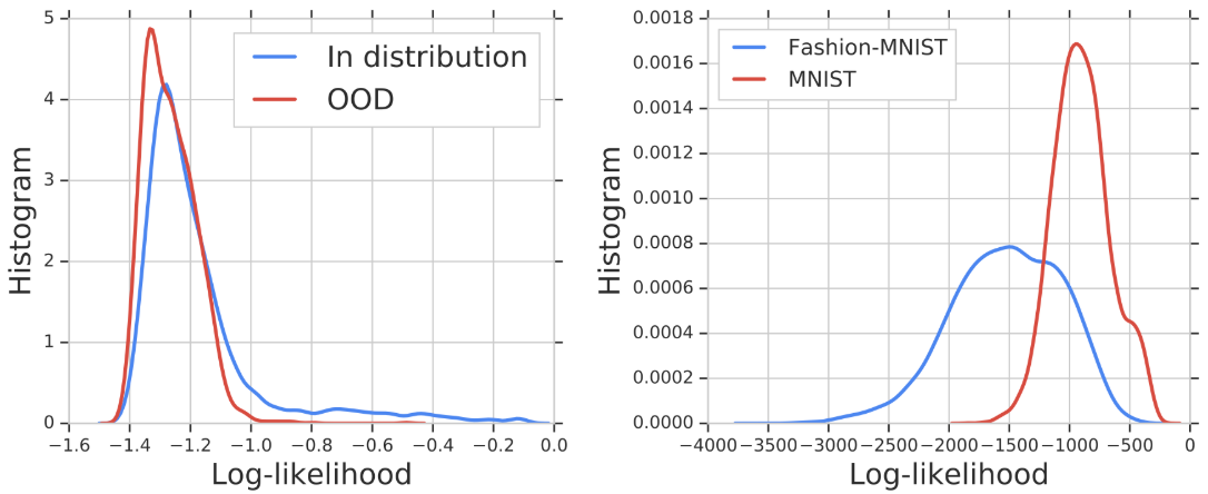 |
| Left: Histogram of likelihood values for in- and out-of-distribution (OOD) genomic sequences. The likelihood fails to separate in-distribution and OOD genomic sequences. Right: A similar plot for a model trained on Fashion-MNIST and evaluated on MNIST. The model assigns higher likelihood values for OOD (MNIST) than in-distribution images. |
When investigating this failure mode, we observed that the likelihood can be confounded by background statistics. To understand the phenomenon more intuitively, assume that an input is composed of two components, (1) a background component characterized by background statistics, and (2) a semantic component characterized by patterns specific to the in-distribution data. For example, an MNIST image can be modeled as background plus semantics. When humans interpret the image, we can easily ignore the background and focus primarily on the semantic information, e.g., the “/” mark in the image below. But the likelihood is calculated for all pixels in an image, including both semantic and background pixels. Though we want to use just the semantic likelihood for decision making, the raw likelihood can be dominated by background.
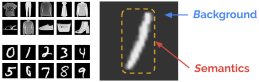 |
| Left top: Sample images from Fashion-MNIST. Left bottom: Sample images from MNIST. Right: Background and semantic components in an MNIST image. |
Likelihood Ratios For OOD Detection
We propose a likelihood ratio method that removes the effect of background and focuses on semantics. First, we train a background model on perturbed inputs. The method for perturbing the input is inspired by genetic mutations, and proceeds by randomly selecting positions in the input and substituting the value with another that has equal probability. For imaging, the values are randomly chosen from the 256 possible pixel values, and for the DNA sequences, the value is selected from the four possible nucleotides (A, T, C, or G). The right amount of perturbation can corrupt the semantic structure in the data, and captures only the background. Then we compute the likelihood ratio between the full model and the background model, and the background component is cancelled out, so that only the likelihood for semantics remains. Likelihood ratio is a background contrastive score, i.e., it captures the significance of the semantics compared to the background.
To qualitatively evaluate the difference between the likelihood and likelihood ratio, we plotted their values for each pixel in the Fashion-MNIST and MNIST datasets, creating heatmaps that have the same size as the images. This allows us to visualize which pixels contribute the most to the two terms, respectively. From the log-likelihood heatmaps, we see that the background pixels contribute much more to the likelihood than the semantic pixels. In hindsight, this is not surprising, since background pixels consist mostly of a string of zeros, a pattern very easily learned by the model. A comparison between the MNIST and Fashion-MNIST heatmaps demonstrates why MNIST returns higher likelihood values — it simply has a lot more background pixels! The likelihood ratio instead focuses more on the semantic pixels.
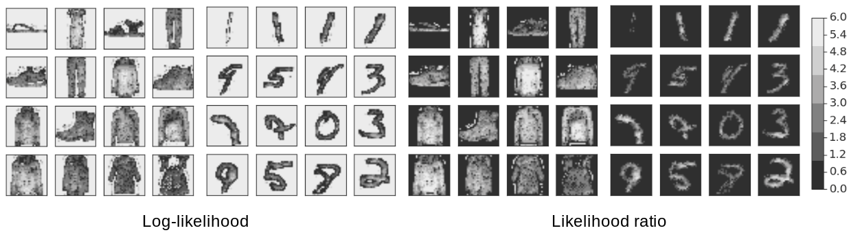 |
| Left: Log-likelihood heatmaps for Fashion-MNIST and MNIST datasets. Right: The same examples showing heatmaps of the likelihood-ratio. Pixels with higher values are of lighter shades. The likelihood is dominated by the “background” pixels, whereas the likelihood ratio focuses on the “semantic” pixels and is thus better for OOD detection. |
Our likelihood ratio method corrects the background effect and significantly improves the OOD detection of MNIST images from an AUROC score of 0.089 to 0.994, based on a PixelCNN++ model trained for Fashion-MNIST. When applied to the genomic benchmark dataset, this method achieves state-of-the-art performance on this challenging problem, when compared to 12 other baseline methods.
For more details, please check out our recent paper at NeurIPS 2019. While our likelihood ratio method reaches state-of-the-art performance on the genomic dataset, it does not yet have high enough accuracy to reach the standards for deployment of the model to real applications. We encourage researchers to contribute their solutions to this important problem and improve the current state-of-the-art. The dataset is available on our GitHub repository.
Acknowledgments
The work described here was authored by Jie Ren, Peter J. Liu, Emily Fertig, Jasper Snoek, Ryan Poplin, Mark A. DePristo, Joshua V. Dillon, Balaji Lakshminarayanan, through a collaboration spanning several teams across Google AI and DeepMind. We are grateful for all the discussions and feedback on this work that we received from the reviewers at NeurIPS 2019, and our colleagues at Google and DeepMind: Alexander A. Alemi, Andreea Gane, Brian Lee, D. Sculley, Eric Jang, Jacob Burnim, Katherine Lee, Matthew D. Hoffman, Noah Fiedel, Rif A. Saurous, Suman Ravuri, Thomas Colthurst, Yaniv Ovadia, along with the Google Brain and TensorFlow teams.
