Multi Class Text Classification with LSTM using TensorFlow 2.0
Recurrent Neural Networks, Long Short Term Memory
A lot of innovations on NLP have been how to add context into word vectors. One of the common ways of doing it is using Recurrent Neural Networks. The following are the concepts of Recurrent Neural Networks:
- They make use of sequential information.
- They have a memory that captures what have been calculated so far, i.e. what I spoke last will impact what I will speak next.
- RNNs are ideal for text and speech analysis.
- The most commonly used RNNs are LSTMs.

The above is the architecture of Recurrent Neural Networks.
- “A” is one layer of feed-forward neural network.
- If we only look at the right side, it does recurrently to pass through the element of each sequence.
- If we unwrap the left, it will exactly look like the right.

Assuming we are solving document classification problem for a news article data set.
- We input each word, words relate to each other in some ways.
- We make predictions at the end of the article when we see all the words in that article.
- RNNs, by passing input from last output, are able to retain information, and able to leverage all information at the end to make predictions.

- This works well for short sentences, when we deal with a long article, there will be a long term dependency problem.
Therefore, we generally do not use vanilla RNNs, and we use Long Short Term Memory instead. LSTM is a type of RNNs that can solve this long term dependency problem.

In our document classification for news article example, we have this many-to- one relationship. The input are sequences of words, output is one single class or label.
Now we are going to solve a BBC news document classification problem with LSTM using TensorFlow 2.0 & Keras. The data set can be found here.
- First, we import the libraries and make sure our TensorFlow is the right version.
https://medium.com/media/c3ce0e6b10a84a676c3d9de30e90b1fb/href

- Put the hyperparameters at the top like this to make it easier to change and edit.
- We will explain how each hyperparameter works when we get there.
https://medium.com/media/7f3901aa39de489d143a5b733a09ff9c/href
- Define two lists containing articles and labels. In the meantime, we remove stopwords.
https://medium.com/media/78a4697725a3ec5f5861866ffd32cc56/href

There are 2,225 news articles in the data, we split them into training set and validation set, according to the parameter we set earlier, 80% for training, 20% for validation.
https://medium.com/media/87df8873bbd3b423c283bf3855fcb002/href
Tokenizer does all the heavy lifting for us. In our articles that it was tokenizing, it will take 5,000 most common words. oov_token is to put a special value in when an unseen word is encountered. This means we want <OOV> to be used for words that are not in the word_index. fit_on_text will go through all the text and create dictionary like this:
https://medium.com/media/cef356057de89bd5541b5537c2baeb8b/href

We can see that “<OOV>” is the most common token in our corpus, followed by “said”, followed by “mr” and so on.
After tokenization, the next step is to turn those tokens into lists of sequence. The following is the 11th article in the training data that has been turned into sequences.
train_sequences = tokenizer.texts_to_sequences(train_articles)
print(train_sequences[10])

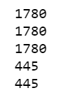
When we train neural networks for NLP, we need sequences to be in the same size, that’s why we use padding. If you look up, our max_length is 200, so we use pad_sequences to make all of our articles the same length which is 200. As a result, you will see that the 1st article was 426 in length, it becomes 200, the 2nd article was 192 in length, it becomes 200, and so on.
train_padded = pad_sequences(train_sequences, maxlen=max_length, padding=padding_type, truncating=trunc_type)
print(len(train_sequences[0]))
print(len(train_padded[0]))

print(len(train_sequences[1]))
print(len(train_padded[1]))

print(len(train_sequences[10]))
print(len(train_padded[10]))

In addition, there is padding_type and truncating_type, there are all post, means for example, for the 11th article, it was 186 in length, we padded to 200, and we padded at the end, that is adding 14 zeros.
print(train_padded[10])
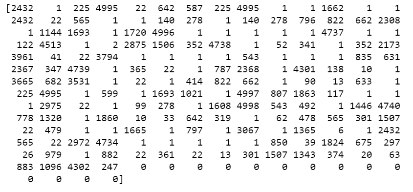
And for the 1st article, it was 426 in length, we truncated to 200, and we truncated at the end as well.
Then we do the same for the validation sequences.
https://medium.com/media/c43e36bb81b9b4fdea972e2ebdb2068c/href

Now we are going to look at the labels. Because our labels are text, so we will tokenize them, when training, labels are expected to be numpy arrays. So we will turn list of labels into numpy arrays like so:
label_tokenizer = Tokenizer()
label_tokenizer.fit_on_texts(labels)

training_label_seq = np.array(label_tokenizer.texts_to_sequences(train_labels))
validation_label_seq = np.array(label_tokenizer.texts_to_sequences(validation_labels))
print(training_label_seq[0])
print(training_label_seq[1])
print(training_label_seq[2])
print(training_label_seq.shape)

print(validation_label_seq[0])
print(validation_label_seq[1])
print(validation_label_seq[2])
print(validation_label_seq.shape)

Before training deep neural network, we should explore what our original article and article after padding look like. Running the following code, we explore the 11th article, we can see that some words become “<OOV>”, because they did not make to the top 5,000.
reverse_word_index = dict([(value, key) for (key, value) in word_index.items()])

def decode_article(text):
return ' '.join([reverse_word_index.get(i, '?') for i in text])
print(decode_article(train_padded[10]))
print('---')
print(train_articles[10])

Now its the time to implement LSTM.
- We build a tf.keras.Sequential model and start with an embedding layer. An embedding layer stores one vector per word. When called, it converts the sequences of word indices into sequences of vectors. After training, words with similar meanings often have the similar vectors.
- The Bidirectional wrapper is used with a LSTM layer, this propagates the input forwards and backwards through the LSTM layer and then concatenates the outputs. This helps LSTM to learn long term dependencies. We then fit it to a dense neural network to do classification.
- We use relu in place of tahn function since they are very good alternatives of each other.
- We add a Dense layer with 6 units and softmax activation. When we have multiple outputs, softmax converts outputs layers into a probability distribution.
https://medium.com/media/928f6aee4451f31480029ddb8efd7cf6/href
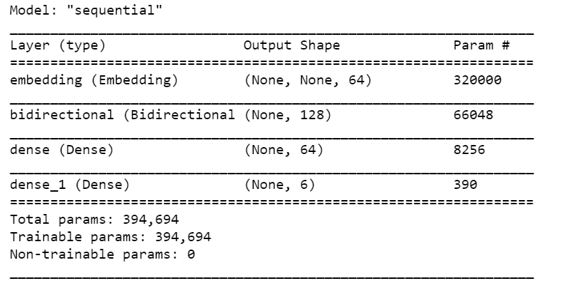
In our model summary, we have our embeddings, our Bidirectional contains LSTM, followed by two dense layers. The output from Bidirectional is 128, because it doubled what we put in LSTM. We can also stack LSTM layer but I found the results worse.
print(set(labels))

We have 5 labels in total, but because we did not one-hot encode labels, we have to use sparse_categorical_crossentropy as loss function, it seems to think 0 is a possible label as well, while the tokenizer object which tokenizes starting with integer 1, instead of integer 0. As a result, the last Dense layer needs outputs for labels 0, 1, 2, 3, 4, 5 although 0 has never been used.
If you want the last Dense layer to be 5, you will need to subtract 1 from the training and validation labels. I decided to leave it as it is.
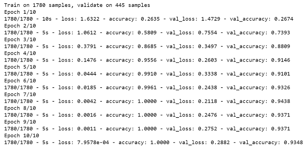
I decided to train 10 epochs, and it is plenty of epochs as you will see.
model.compile(loss='sparse_categorical_crossentropy', optimizer='adam', metrics=['accuracy'])
num_epochs = 10
history = model.fit(train_padded, training_label_seq, epochs=num_epochs, validation_data=(validation_padded, validation_label_seq), verbose=2)
def plot_graphs(history, string):
  plt.plot(history.history[string])
  plt.plot(history.history['val_'+string])
  plt.xlabel("Epochs")
  plt.ylabel(string)
  plt.legend([string, 'val_'+string])
  plt.show()

plot_graphs(history, "accuracy")
plot_graphs(history, "loss")

We probably only need 3 or 4 epochs. At the end of the training, we can see that there is a little bit overfitting.
In the future posts, we will work on improving the model.
Jupyter notebook can be found on Github. Enjoy the rest of the weekend!
References:
- Coursera | Online Courses From Top Universities. Join for Free
- O’Reilly Strata Data Conference 2019 – New York, New York
Multi Class Text Classification with LSTM using TensorFlow 2.0 was originally published in Towards Data Science on Medium, where people are continuing the conversation by highlighting and responding to this story.