Deep learning, text classification, NLP

This article shows how to use a simple LSTM and one of the pre-trained GloVe files to create a strong baseline for the toxic comments classification problem.

The article consist of 4 main sections:

• Preparing the data
• Implementing a simple LSTM (RNN) model
• Training the model
• Evaluating the model

The Data

In the following steps, we will set the key model parameters and split the data.

• “MAX_NB_WORDS” sets the maximum number of words to consider as features for tokenizer.
• “MAX_SEQUENCE_LENGTH” cuts off texts after this number of words (among the MAX_NB_WORDS most common words).
• “VALIDATION_SPLIT” sets a portion of data for validation and not used in training.
• “EMBEDDING_DIM” defines the size of the “vector space”.
• “GLOVE_DIR” defines the GloVe file directory.
• Split the data into the texts and the labels.

https://medium.com/media/e404f87284057d710e0e0f3967897354/href

Text Pre-processing

In the following step, we remove stopwords, punctuation and make everything lowercase.

https://medium.com/media/eadbd6070963e87f8225525edc19beff/href

Have a look a sample data.

print('Sample data:', texts[1], y[1])

• We create a tokenizer, configured to only take into account the MAX_NB_WORDS most common words.
• We build the word index.
• We can recover the word index that was computed.

tokenizer = Tokenizer(num_words=MAX_NB_WORDS)
tokenizer.fit_on_texts(texts)
sequences = tokenizer.texts_to_sequences(texts)
word_index = tokenizer.word_index
print('Vocabulary size:', len(word_index))

• Turns the lists of integers into a 2D integer tensor of shape (samples, maxlen)
• Pad after each sequence.

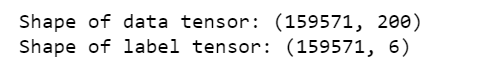
data = pad_sequences(sequences, padding = 'post', maxlen = MAX_SEQUENCE_LENGTH)

print('Shape of data tensor:', data.shape)
print('Shape of label tensor:', y.shape)

• Shuffle the data.

indices = np.arange(data.shape[0])
np.random.shuffle(indices)
data = data[indices]
labels = y[indices]

Create the train-validation split.

num_validation_samples = int(VALIDATION_SPLIT*data.shape[0])
x_train = data[: -num_validation_samples]
y_train = labels[: -num_validation_samples]
x_val = data[-num_validation_samples: ]
y_val = labels[-num_validation_samples: ]

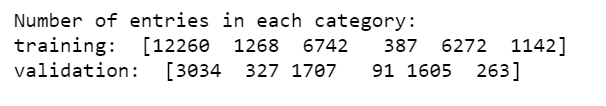
print('Number of entries in each category:')
print('training: ', y_train.sum(axis=0))
print('validation: ', y_val.sum(axis=0))

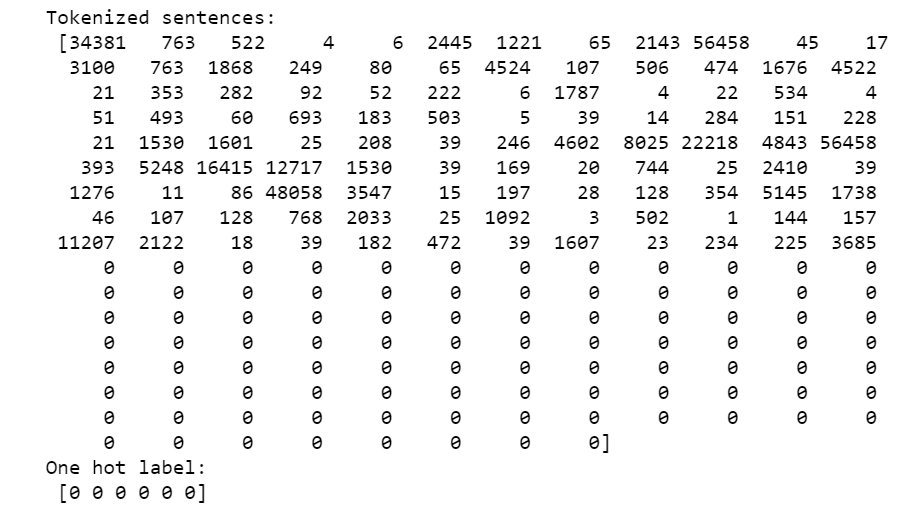
This is what the data looks like:

print('Tokenized sentences: n', data[10])
print('One hot label: n', labels[10])

Create the model

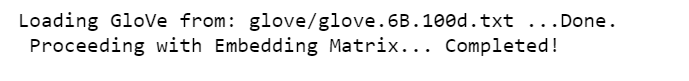
• We will use pre-trained GloVe vectors from Stanford to create an index of words mapped to known embeddings, by parsing the data dump of pre-trained embeddings.
• Then load word embeddings into an embeddings_index

https://medium.com/media/4a58a99c42bc4a3760b0155be6d63f59/href

• Create the embedding layers.
• Specifies the maximum input length to the Embedding layer.
• Make use of the output from the previous embedding layer which outputs a 3-D tensor into the LSTM layer.
• Use a Global Max Pooling layer to to reshape the 3D tensor into a 2D one.
• We set the dropout layer to drop out 10% of the nodes.
• We define the Dense layer to produce a output dimension of 50.
• We feed the output into a Dropout layer again.
• Finally, we feed the output into a “Sigmoid” layer.

https://medium.com/media/6d48566a561c43069f9da57f9ad9e800/href

Its time to Compile the model into a static graph for training.

• Define the inputs, outputs and configure the learning process.
• Set the model to optimize our loss function using “Adam” optimizer, define the loss function to be “binary_crossentropy” .

model = Model(sequence_input, preds)
model.compile(loss = 'binary_crossentropy',
             optimizer='adam',
             metrics = ['accuracy'])

Training

• Feed in a list of 32 padded, indexed sentence for each batch. The validation set will be used to assess whether the model has overfitted.
• The model will run for 2 epochs, because even 2 epochs is enough to overfit.

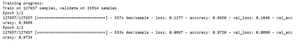
print('Training progress:')
history = model.fit(x_train, y_train, epochs = 2, batch_size=32, validation_data=(x_val, y_val))

Evaluate the model

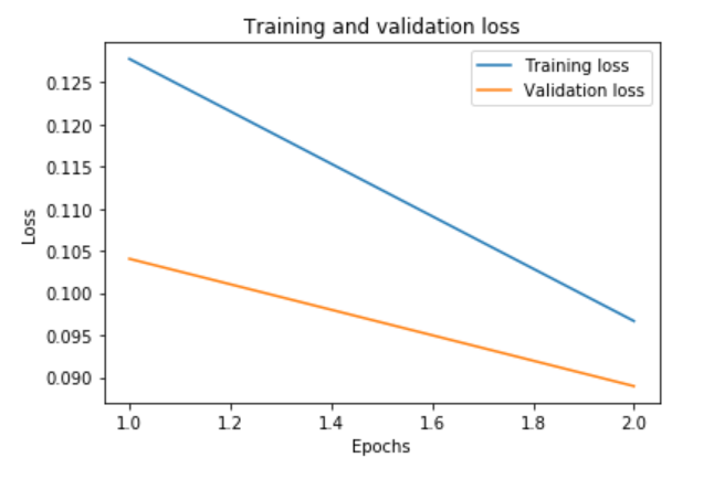
loss = history.history['loss']
val_loss = history.history['val_loss']

epochs = range(1, len(loss)+1)

plt.plot(epochs, loss, label='Training loss')
plt.plot(epochs, val_loss, label='Validation loss')
plt.title('Training and validation loss')
plt.xlabel('Epochs')
plt.ylabel('Loss')
plt.legend()
plt.show();

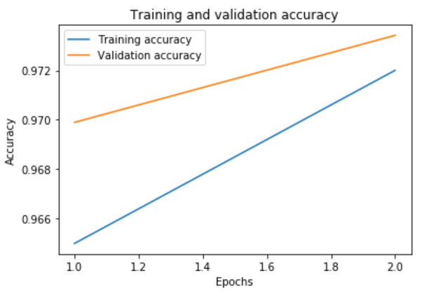
accuracy = history.history['accuracy']
val_accuracy = history.history['val_accuracy']

plt.plot(epochs, accuracy, label='Training accuracy')
plt.plot(epochs, val_accuracy, label='Validation accuracy')
plt.title('Training and validation accuracy')
plt.ylabel('Accuracy')
plt.xlabel('Epochs')
plt.legend()
plt.show();

Jupyter notebook can be found on Github. Happy Monday!

Classify Toxic Online Comments with LSTM and GloVe was originally published in Towards Data Science on Medium, where people are continuing the conversation by highlighting and responding to this story.