Figure: An artistic representation of single-cell RNA sequencing. The
stars in the sky represent cells in a heterogeneous tissue. The projection of
the stars onto the river reveals relationships among them that are not apparent
by looking directly at the sky. Like the river, our Bayesian model, called scVI,
reveals relationships among cells.
The diversity of gene regulatory states in our body is one of the main reasons
why such an amazing array of biological functions can be encoded in a single
genome. Recent advances in microfluidics and sequencing technologies (such as inDrops) enabled measurement of gene expression at the single-cell level and has
provided tremendous opportunities to unravel the underlying mechanisms of
relationships between individual genes and specific biological phenomena. These
experiments yield approximate measurements for mRNA counts of the entire
transcriptome (i.e around $d = 20,000$ protein-coding genes) and a large number
of cells $n$, which can vary from tens of thousands to a million cells. The
early computational methods to interpret this data relied on linear model and
empirical Bayes shrinkage approaches due to initially extremely low sample-size.
While current research focuses on providing more accurate models for this gene
expression data, most of the subsequent algorithms either exhibit prohibitive
scalability issues or remain limited to a unique downstream analysis task.
Consequently, common practices in the field still rely on ad-hoc preprocessing
pipelines and specific algorithmic procedures, which limits the capabilities of
capturing the underlying data generating process.
In this post, we propose to build up on the increased sample-size and recent
developments in Bayesian approximate inference to improve modeling complexity as
well as algorithmic scalability. Notably, we present our recent work on deep
generative models for single-cell transcriptomics, which addresses all the
mentioned limitations by formalizing biological questions into statistical
queries over a unique graphical model, tailored to single-cell RNA sequencing
(scRNA-seq) datasets. The resulting algorithmic inference procedure, which we
named Single-cell Variational Inference (scVI), is open-source and
scales to over a million cells.
With very little explicit supervision and feedback, humans are able to learn a
wide range of motor skills by simply interacting with and observing the world
through their senses. While there has been significant progress towards building
machines that can learn complex
skills and learn
based on raw sensory information such as image pixels, acquiring large and
diverse repertoires of general skills remains an open challenge. Our goal is
to build a generalist: a robot that can perform many different tasks, like
arranging objects, picking up toys, and folding towels, and can do so with many
different objects in the real world without re-learning for each object or task.
While these basic motor skills are much simpler and less impressive than mastering Chess or even using a spatula, we think that
being able to achieve such generality with a single model is a fundamental
aspect of intelligence.
The key to acquiring generality is diversity. If you deploy a learning
algorithm in a narrow, closed-world environment, the agent will recover skills
that are successful only in a narrow range of settings. That’s why an algorithm
trained to play Breakout will struggle when anything about the images or the
game changes. Indeed, the success of image classifiers relies on large, diverse
datasets like ImageNet. However, having a robot autonomously learn from large
and diverse datasets is quite challenging. While collecting diverse sensory data
is relatively straightforward, it is simply not practical for a person to
annotate all of the robot’s experiences. It is more scalable to collect
completely unlabeled experiences. Then, given only sensory data, akin to what
humans have, what can you learn? With raw sensory data there is no notion of
progress, reward, or success. Unlike games like Breakout, the real world doesn’t
give us a score or extra lives.
We have developed an algorithm that can learn a general-purpose predictive model
using unlabeled sensory experiences, and then use this single model to perform a
wide range of tasks.
With a single model, our approach can perform a wide range of tasks, including
lifting objects, folding shorts, placing an apple onto a plate, rearranging
objects, and covering a fork with a towel.
In this post, we will describe how this works. We will discuss how we can learn
based on only raw sensory interaction data (i.e. image pixels, without requiring
object detectors or hand-engineered perception components). We will show how we
can use what was learned to accomplish many different user-specified tasks. And,
we will demonstrate how this approach can control a real robot from raw pixels,
performing tasks and interacting with objects that the robot has never seen
before.
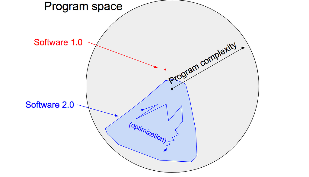
I sometimes see people refer to neural networks as just “another tool in your machine learning toolbox”. They have some pros and cons, they work here or there, and sometimes you can use them to win Kaggle competitions. Unfortunately, this interpretation completely misses the forest for the trees. Neural networks are not just another classifier, they represent the beginning of a fundamental shift in how we write software. They are Software 2.0.
The “classical stack” of Software 1.0 is what we’re all familiar with — it is written in languages such as Python, C++, etc. It consists of explicit instructions to the computer written by a programmer. By writing each line of code, the programmer identifies a specific point in program space with some desirable behavior.
In contrast, Software 2.0 can be written in much more abstract, human unfriendly language, such as the weights of a neural network. No human is involved in writing this code because there are a lot of weights (typical networks might have millions), and coding directly in weights is kind of hard (I tried).
Instead, our approach is to specify some goal on the behavior of a desirable program (e.g., “satisfy a dataset of input output pairs of examples”, or “win a game of Go”), write a rough skeleton of the code (e.g. a neural net architecture), that identifies a subset of program space to search, and use the computational resources at our disposal to search this space for a program that works. In the specific case of neural networks, we restrict the search to a continuous subset of the program space where the search process can be made (somewhat surprisingly) efficient with backpropagation and stochastic gradient descent.
It turns out that a large portion of real-world problems have the property that it is significantly easier to collect the data (or more generally, identify a desirable behavior) than to explicitly write the program. In these cases, the programmers will split into two teams. The 2.0 programmers manually curate, maintain, massage, clean and label datasets; each labeled example literally programs the final system because the dataset gets compiled into Software 2.0 code via the optimization. Meanwhile, the 1.0 programmers maintain the surrounding tools, analytics, visualizations, labeling interfaces, infrastructure, and the training code.
Ongoing transition
Let’s briefly examine some concrete examples of this ongoing transition. In each of these areas we’ve seen improvements over the last few years when we give up on trying to address a complex problem by writing explicit code and instead transition the code into the 2.0 stack.
Visual Recognition used to consist of engineered features with a bit of machine learning sprinkled on top at the end (e.g., an SVM). Since then, we discovered much more powerful visual features by obtaining large datasets (e.g. ImageNet) and searching in the space of Convolutional Neural Network architectures. More recently, we don’t even trust ourselves to hand-code the architectures and we’ve begun searching over those as well.
Speech recognition used to involve a lot of preprocessing, gaussian mixture models and hidden markov models, but today consist almost entirely of neural net stuff. A very related, often cited humorous quote attributed to Fred Jelinek from 1985 reads “Every time I fire a linguist, the performance of our speech recognition system goes up”.
Speech synthesis has historically been approached with various stitching mechanisms, but today the state of the art models are large ConvNets (e.g. WaveNet) that produce raw audio signal outputs.
Machine Translation has usually been approaches with phrase-based statistical techniques, but neural networks are quickly becoming dominant. My favorite architectures are trained in the multilingual setting, where a single model translates from any source language to any target language, and in weakly supervised (or entirely unsupervised) settings.
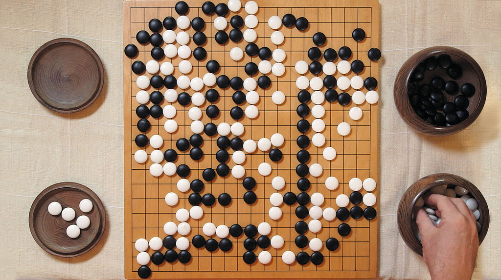
Games. Explicitly hand-coded Go playing programs have been developed for a long while, but AlphaGo Zero (a ConvNet that looks at the raw state of the board and plays a move) has now become by far the strongest player of the game. I expect we’re going to see very similar results in other areas, e.g. DOTA 2, or StarCraft.
Databases. More traditional systems outside of Artificial Intelligence are also seeing early hints of a transition. For instance, “The Case for Learned Index Structures” replaces core components of a data management system with a neural network, outperforming cache-optimized B-Trees by up to 70% in speed while saving an order-of-magnitude in memory.
You’ll notice that many of my links above involve work done at Google. This is because Google is currently at the forefront of re-writing large chunks of itself into Software 2.0 code. “One model to rule them all” provides an early sketch of what this might look like, where the statistical strength of the individual domains is amalgamated into one consistent understanding of the world.
The benefits of Software 2.0
Why should we prefer to port complex programs into Software 2.0? Clearly, one easy answer is that they work better in practice. However, there are a lot of other convenient reasons to prefer this stack. Let’s take a look at some of the benefits of Software 2.0 (think: a ConvNet) compared to Software 1.0 (think: a production-level C++ code base). Software 2.0 is:
Computationally homogeneous. A typical neural network is, to the first order, made up of a sandwich of only two operations: matrix multiplication and thresholding at zero (ReLU). Compare that with the instruction set of classical software, which is significantly more heterogenous and complex. Because you only have to provide Software 1.0 implementation for a small number of the core computational primitives (e.g. matrix multiply), it is much easier to make various correctness/performance guarantees.
Simple to bake into silicon. As a corollary, since the instruction set of a neural network is relatively small, it is significantly easier to implement these networks much closer to silicon, e.g. with custom ASICs, neuromorphic chips, and so on. The world will change when low-powered intelligence becomes pervasive around us. E.g., small, inexpensive chips could come with a pretrained ConvNet, a speech recognizer, and a WaveNet speech synthesis network all integrated in a small protobrain that you can attach to stuff.
Constant running time. Every iteration of a typical neural net forward pass takes exactly the same amount of FLOPS. There is zero variability based on the different execution paths your code could take through some sprawling C++ code base. Of course, you could have dynamic compute graphs but the execution flow is normally still significantly constrained. This way we are also almost guaranteed to never find ourselves in unintended infinite loops.
Constant memory use. Related to the above, there is no dynamically allocated memory anywhere so there is also little possibility of swapping to disk, or memory leaks that you have to hunt down in your code.
It is highly portable. A sequence of matrix multiplies is significantly easier to run on arbitrary computational configurations compared to classical binaries or scripts.
It is very agile. If you had a C++ code and someone wanted you to make it twice as fast (at cost of performance if needed), it would be highly non-trivial to tune the system for the new spec. However, in Software 2.0 we can take our network, remove half of the channels, retrain, and there — it runs exactly at twice the speed and works a bit worse. It’s magic. Conversely, if you happen to get more data/compute, you can immediately make your program work better just by adding more channels and retraining.
Modules can meld into an optimal whole. Our software is often decomposed into modules that communicate through public functions, APIs, or endpoints. However, if two Software 2.0 modules that were originally trained separately interact, we can easily backpropagate through the whole. Think about how amazing it could be if your web browser could automatically re-design the low-level system instructions 10 stacks down to achieve a higher efficiency in loading web pages. With 2.0, this is the default behavior.
It is better than you. Finally, and most importantly, a neural network is a better piece of code than anything you or I can come up with in a large fraction of valuable verticals, which currently at the very least involve anything to do with images/video and sound/speech.
The limitations of Software 2.0
The 2.0 stack also has some of its own disadvantages. At the end of the optimization we’re left with large networks that work well, but it’s very hard to tell how. Across many applications areas, we’ll be left with a choice of using a 90% accurate model we understand, or 99% accurate model we don’t.
The 2.0 stack can fail in unintuitive and embarrassing ways ,or worse, they can “silently fail”, e.g., by silently adopting biases in their training data, which are very difficult to properly analyze and examine when their sizes are easily in the millions in most cases.
Finally, we’re still discovering some of the peculiar properties of this stack. For instance, the existence of adversarial examples and attacks highlights the unintuitive nature of this stack.
Programming in the 2.0 stack
Software 1.0 is code we write. Software 2.0 is code written by the optimization based on an evaluation criterion (such as “classify this training data correctly”). It is likely that any setting where the program is not obvious but one can repeatedly evaluate the performance of it (e.g. — did you classify some images correctly? do you win games of Go?) will be subject to this transition, because the optimization can find much better code than what a human can write.
The lens through which we view trends matters. If you recognize Software 2.0 as a new and emerging programming paradigm instead of simply treating neural networks as a pretty good classifier in the class of machine learning techniques, the extrapolations become more obvious, and it’s clear that there is much more work to do.
In particular, we’ve built up a vast amount of tooling that assists humans in writing 1.0 code, such as powerful IDEs with features like syntax highlighting, debuggers, profilers, go to def, git integration, etc. In the 2.0 stack, the programming is done by accumulating, massaging and cleaning datasets. For example, when the network fails in some hard or rare cases, we do not fix those predictions by writing code, but by including more labeled examples of those cases. Who is going to develop the first Software 2.0 IDEs, which help with all of the workflows in accumulating, visualizing, cleaning, labeling, and sourcing datasets? Perhaps the IDE bubbles up images that the network suspects are mislabeled based on the per-example loss, or assists in labeling by seeding labels with predictions, or suggests useful examples to label based on the uncertainty of the network’s predictions.
Similarly, Github is a very successful home for Software 1.0 code. Is there space for a Software 2.0 Github? In this case repositories are datasets and commits are made up of additions and edits of the labels.
In the short/medium term, Software 2.0 will become increasingly prevalent in any domain where repeated evaluation is possible and cheap, and where the algorithm itself is difficult to design explicitly. And in the long run, the future of this paradigm is bright because it is increasingly clear to many that when we develop AGI, it will certainly be written in Software 2.0.
there’s something subtle also going on in the objective with the entropy regularization, which is inserted into policy gradients to incetivise exploration.
The side of effect of this is that the optimal agent behavior will actually be to act randomly when it doesn’t matter. In Pong, the final agent therefore jitters around randomly with maximum entropy, but when it comes to catching the ball, executing the precise sequence of moves needed to get that done. And then reverting back to random behavior.
Update Oct 18, 2017: AlphaGo Zero was announced. This post refers to the previous version. 95% of it still applies.
I had a chance to talk to several people about the recent AlphaGo matches with Ke Jie and others. In particular, most of the coverage was a mix of popular science + PR so the most common questions I’ve seen were along the lines of “to what extent is AlphaGo a breakthrough?”, “How do researchers in AI see its victories?” and “what implications do the wins have?”. I thought I might as well serialize some of my thoughts into a post.
The cool parts
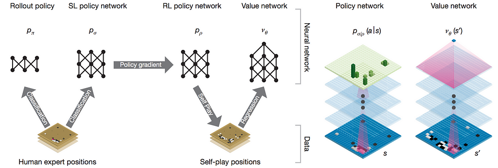
AlphaGo is made up of a number of relatively standard techniques: behavior cloning (supervised learning on human demonstration data), reinforcement learning (REINFORCE), value functions, and Monte Carlo Tree Search (MCTS). However, the way these components are combined is novel and not exactly standard. In particular, AlphaGo uses a SL (supervised learning) policy to initialize the learning of an RL (reinforcement learning) policy that gets perfected with self-play, which they then estimate a value function from, which then plugs into MCTS that (somewhat surprisingly) uses the (worse!, but more diverse) SL policy to sample rollouts. In addition, the policy/value nets are deep neural networks, so getting everything to work properly presents its own unique challenges (e.g. value function is trained in a tricky way to prevent overfitting). On all of these aspects, DeepMind has executed very well. That being said, AlphaGo does not by itself use any fundamental algorithmic breakthroughs in how we approach RL problems.
On narrowness
Zooming out, it is also still the case that AlphaGo is a narrow AI system that can play Go and that’s it. The ATARI-playing agents from DeepMind do not use the approach taken with AlphaGo. The Neural Turing Machine has little to do with AlphaGo. The Google datacenter improvements definitely do not use AlphaGo. The Google Search engine is not going to use AlphaGo. Therefore, AlphaGo does not generalize to any problem outside of Go, but the people and the underlying neural network components do, and do so much more effectively than in the days of old AI where each demonstration needed repositories of specialized, explicit code.
Convenient properties of Go
I wanted to expand on the narrowness of AlphaGo by explicitly trying to list some of the specific properties that Go has, which AlphaGo benefits a lot from. This can help us think about what settings AlphaGo does or does not generalize to. Go is:
fully deterministic. There is no noise in the rules of the game; if the two players take the same sequence of actions, the states along the way will always be the same.
fully observed. Each player has complete information and there are no hidden variables. For example, Texas hold’em does not satisfy this property because you cannot see the cards of the other player.
the action space is discrete. a number of unique moves are available. In contrast, in robotics you might want to instead emit continuous-valued torques at each joint.
we have access to a perfect simulator (the game itself), so the effects of any action are known exactly. This is a strong assumption that AlphaGo relies on quite strongly, but is also quite rare in other real-world problems.
each episode/game is relatively short, of approximately 200 actions. This is a relatively short time horizon compared to other RL settings which may involve thousands (or more) of actions per episode.
the evaluation is clear, fast and allows a lot of trial-and-error experience. In other words, the agentcan experience winning/losing millions of times, which allows is to learn, slowly but surely, as is common with deep neural network optimization.
there are huge datasets of human play game data available to bootstrap the learning, so AlphaGo doesn’t have to start from scratch.
Example: AlphaGo applied to robotics?
Having enumerated some of the appealing properties of Go, let’s look at a robotics problem and see how well we could apply AlphaGo to, for example, an Amazon Picking Challenge robot. It’s a little comical to even think about.
First, your (high-dimensional, continuous) actions are awkwardly /noisily executed by the robot’s motors (1,3 are violated).
The robot might have to look around for the items that are to be moved, so it doesn’t always sense all the relevant information and has to sometimes collect it on demand. (2 is violated)
We might have a physics simulator, but these are quite imperfect (especially for simulating things like contact forces); this brings its own set of non-trivial challenges (4 is violated).
Depending on how abstract your action space is (raw torques -> positions of the gripper), a successful episode can be much longer than 200 actions (i.e. 5 depends on the setting). Longer episodes add to the credit assignment problem, where it is difficult for the learning algorithm to distribute blame among the actions for any outcome.
It would be much harder for a robot to practice (succeed/fail) at something millions of times, because we’re operating in the real world. One approach might be to parallelize robots, but that can be quite expensive. Also, a robot failing might involve the robot actually damaging itself. Another approach would be to use a simulator and then transfer to the real world, but this brings its own set of new, non-trivial challenges in the domain transfer. Lastly, in many cases evaluation is very non-trivial. For example, how do you automatically evaluate if a robot has succeeded in making an omelette? (6 is violated).
There is rarely a human data source with millions of demonstrations (so 7 is violated).
In short, basically every single assumption that Go satisfies and that AlphaGo takes advantage of are violated, and any successful approach would look extremely different. More generally, some of Go’s properties above are not insurmountable with current algorithms (e.g. 1,2,3), some are somewhat problematic (5,7), but some are quite critical to how AlphaGo is trained but are rarely present in other real-world applications (4,6).
In conclusion
While AlphaGo does not introduce fundamental breakthroughs in AI algorithmically, and while it is still an example of narrow AI, AlphaGo does symbolize Alphabet’s AI power: in both the quantity/quality of the talent present in the company, the computational resources at their disposal, and the all in focus on AI from the very top.
Alphabet is making a large bet on AI, and it is a safe one. But I’m biased 🙂
EDIT: the goal of this post is, as someone on reddit mentioned, “quelling the ever resilient beliefs of the public that AGI is right down the road”, and the target audience are people outside of AI who were watching AlphaGo and would like a more technical commentary.
We focus on applying tech to product. Thanks in great part to the open-source movement, it’s easier than ever to build a technology company. However, AI & ML innovation is still in its nascent phase and very hard to apply in the building of comprehensive solutions and scalable products.
We want to make technology accessible. In line with recent announcements made by Google’s CEO Sundar Pichai and Chief Scientist Fei Fei Li, Launchpad is more committed than ever to make new technological advances, like AI and ML, universally accessible and useful to startups globally.
We offer tools and best practices to apply AI to products. With this in mind, Launchpad Studio aims to be a go-to hub for the world’s best AI entrepreneurs by empowering them on their journeys, as they build next-gen products that matter.”
The accepted papers at ICML have been published. ICML is a top Machine Learning conference, and one of the most relevant to Deep Learning, although NIPS has a longer DL tradition and ICLR, being more focused, has a much higher DL density.
Most mentioned institutions
I thought it would be fun to compute some stats on institutions. Armed with Jupyter Notebook and regex, we look for all of the institution mentions, add up their counts and sort. Modulo a few annoyances:
I manually collapse e.g. “Google”, “Google Inc.”, “Google Brain”, “Google Research” into one category, or “Stanford” and “Stanford University”.
I only count up one unique mention of an institution on each paper, so if a paper has 20 people from a single institution this gets collapsed to a single mention. This way we get a better understanding of which institutions are involved on each paper in the conference.
In total we get 961 institution mentions, 420 unique. The top 30 are:
#mentions institution
---------------------
       44 Google
       33 Microsoft
       32 CMU
       25 DeepMind
       23 MIT
       22 Berkeley
       22 Stanford
       16 Cambridge
       16 Princeton
       15 None
       14 Georgia Tech
       13 Oxford
       11 UT Austin
       10 Duke
       10 Facebook
        9 ETH Zurich
        9 EPFL
        8 Columbia
        8 Harvard
        8 Michigan
        7 UCSD
        7 IBM
        7 New York
        7 Peking
        6 Cornell
        6 Washington
        6 Minnesota
        5 Virginia
        5 Weizmann Institute of Science
        5 Microsoft / Princeton / IAS
I’m not quite sure about “None” (15) in there. It’s listed as an institution on the ICML page and I can’t tell if they have a bug or if that’s a real cool new AI institution we don’t yet know about.
Industry vs. Academia
To get an idea of how much of the research is done at industry, I took the counts for the largest industry labs (DeepMind, Google, Microsoft, Facebook, IBM, Disney, Amazon, Adobe) and divide by the total. We get 14%, but this doesn’t capture the looong tail. Looking through the tail, I think it’s fair to say that
about 20–25% of papers have an industry involvement.
or rather, approximately three quarters of all papers at ICML have come entirely out of Academia. Also, since DeepMind/Google are both Alphabet, we can put them together (giving 60 total), and see that
6.3% of ICML papers have a Google/DeepMind author.
It would be fun to run this analysis over time. Back when I started my PhD (~2011), industry research was not as prevalent. It was common to see in Graphics (e.g. Adobe / Disney / etc), but not as much in AI / Machine Learning. A lot of that has changed and from purely subjective observation, the industry involvement has increased dramatically. However, Academia is still doing really well and contributes a large fraction (~75%) of the papers.
cool!
EDIT 1: fixed an error where previously the Alphabet stat above read 10% because I incorrectly added the numbers of DM and Google, instead of properly collapsing them to a single Alphabet entity. EDIT 2: some more discussion and numbers on r/ML thread too.
Google is researching AutoML (Auto Machine Learning) in which it has the ability to change its own architecture directly. This can self test thousands of times to improve overall performance.
From the article: “The AutoML procedure has so far been applied to image recognition and language modeling. Using AI alone, the team have observed it creating programs that are on par with state-of-the-art models designed by the world’s foremost experts on machine learning.”
Have you looked at Google Trends? It’s pretty cool — you enter some keywords and see how Google Searches of that term vary through time. I thought — hey, I happen to have this arxiv-sanity database of 28,303 (arxiv) Machine Learning papers over the last 5 years, so why not do something similar and take a look at how Machine Learning research has evolved over the last 5 years? The results are fairly fun, so I thought I’d post.
(Edit: machine learning is a large area. A good chunk of this post is about deep learning specifically, which is the subarea I am most familiar with.)
The arxiv singularity
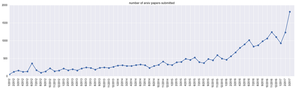
Let’s first look at the total number of submitted papers across the arxiv-sanity categories (cs.AI,cs.LG,cs.CV,cs.CL,cs.NE,stat.ML), over time. We get the following:
Yes, March of 2017 saw almost 2,000 submissions in these areas. The peaks are likely due to conference deadlines (e.g. NIPS/ICML). Note that this is not directly a statement about the size of the area itself, since not everyone submits their paper to arxiv, and the fraction of people who do likely changes over time. But the point remains — that’s a lot of papers to be aware of, skim, or (gasp) read.
This total number of papers will serve as the denominator. We can now look at what fraction of papers contain certain keywords of interest.
Deep Learning Frameworks
To warm up let’s look at the Deep Learning frameworks that are in use. To compute this, we record the fraction of papers that mention the framework somewhere in the full text (anywhere — including bibliography etc). For papers uploaded on March 2017, we get the following:
% of papers 	 framework 	 has been around for (months)
------------------------------------------------------------
    9.1          tensorflow       16
    7.1               caffe       37
    4.6              theano       54
    3.3               torch       37
    2.5               keras       19
    1.7          matconvnet       26
    1.2             lasagne       23
    0.5             chainer       16
    0.3               mxnet       17
    0.3                cntk       13
    0.2             pytorch       1
    0.1      deeplearning4j       14
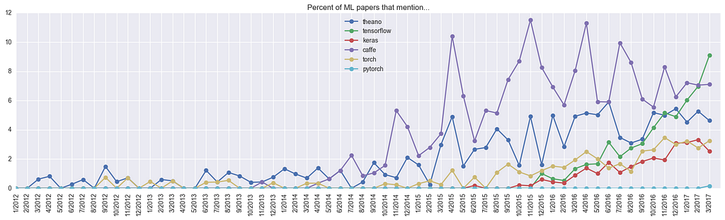
That is, 10% of all papers submitted in March 2017 mention TensorFlow. Of course, not every paper declares the framework used, but if we assume that papers declare the framework with some fixed random probability independent of the framework, then it looks like about 40% of the community is currently using TensorFlow (or a bit more, if you count Keras with the TF backend). And here is the plot of how some of the more popular frameworks evolved over time:
We can see that Theano has been around for a while but its growth has somewhat stalled. Caffe shot up quickly in 2014, but was overtaken by the TensorFlow singularity in the last few months. Torch (and the very recent PyTorch) are also climbing up, slow and steady. It will be fun to watch this develop in the next few months — my own guess is that Caffe/Theano will go on a slow decline and TF growth will become a bit slower due to PyTorch.
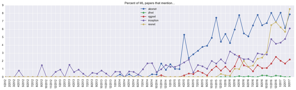
ConvNet Models
For fun, how about if we look at common ConvNet models? Here, we can clearly see a huge spike up for ResNets, to the point that they occur in 9% of all papers last March:
Also, who was talking about “inception” before the InceptionNet? Curious.
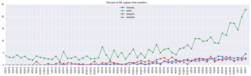
Optimization algorithms
In terms of optimization algorithms, it looks like Adam is on a roll, found in about 23% of papers! The actual fraction of use is hard to estimate; it’s likely higher than 23% because some papers don’t declare the optimization algorithm, and a good chunk of papers might not even be optimizing any neural network at all. It’s then likely lower by about 5%, which is the “background activity” of “Adam”, likely a collision with author names, as the Adam optimization algorithm was only released on Dec 2014.
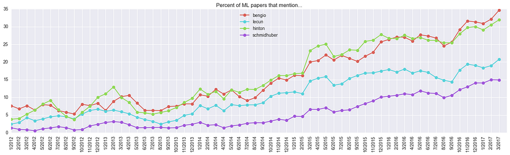
Researchers
I was also curious to plot the mentions of some of the most senior PIs in Deep Learning (this gives something similar to citation count, but 1) it is more robust across population of papers with a “0/1” count, and 2) it is normalized by the total size of the pie):
A few things to note: “bengio” is mentioned in 35% of all submissions, but there are two Bengios: Samy and Yoshua, who add up on this plot. In particular, Geoff Hinton is mentioned in more than 30% of all new papers! That seems like a lot.
Hot or Not Keywords
Finally, instead of manually going by categories of keywords, let’s actively look at the keywords that are “hot” (or not).
Top hot keywords
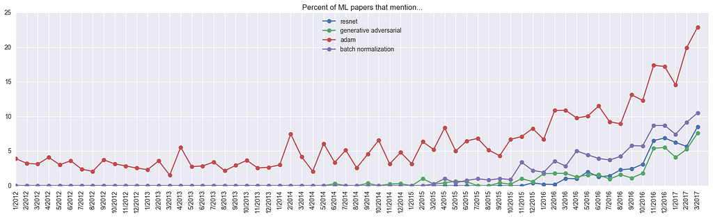
There are many ways to define this, but for this experiment I look at each unigram or bigram in all the papers and record the ratio of its max use last year compared to its max use up to last year. The papers that excel at this metric are those that one year ago were niche, but this year appear with a much higher relative frequency. The top list (slightly edited out some duplicates) comes out as follows:
For example, ResNet’s ratio of 8.17 is because until 1 year ago it appeared in up to only 1.044% of all submissions (in Mar 2016), but last last month (Mar 2017) it appeared in 8.53% of submissions, so 8.53 / 1.044 ~= 8.17. So there you have it — the core innovations that became all the rage over the last year are 1) ResNets, 2) GANs, 3) Adam, 4) BatchNorm. Use more of these to fit in with your friends. In terms of research interests, we see 1) style transfer, 2) deep RL, 3) Neural Machine Translation (“nmt”), and perhaps 4) image generation. And architecturally, it is hot to use 1) Fully Convolutional Nets (FCN), 2) LSTMs/GRUs, 3) Siamese nets, and 4) Encoder decoder nets.
Top not hot
How about the reverse? What has seen many fewer submissions over the last year than has historically had a higher “mind share”? Here are a few:
I’m not sure what “fractal” is referring to, but more generally it looks like bayesian nonparametrics are under attack.
Conclusion
Now is the time to submit paper on Fully Convolutional Encoder Decoder BatchNorm ResNet GAN applied to Style Transfer, optimized with Adam. Hey, that doesn’t even sound too far-fetched.
When we offered CS231n (Deep Learning class) at Stanford, we intentionally designed the programming assignments to include explicit calculations involved in backpropagation on the lowest level. The students had to implement the forward and the backward pass of each layer in raw numpy. Inevitably, some students complained on the class message boards:
“Why do we have to write the backward pass when frameworks in the real world, such as TensorFlow, compute them for you automatically?”
This is seemingly a perfectly sensible appeal – if you’re never going to write backward passes once the class is over, why practice writing them? Are we just torturing the students for our own amusement? Some easy answers could make arguments along the lines of “it’s worth knowing what’s under the hood as an intellectual curiosity”, or perhaps “you might want to improve on the core algorithm later”, but there is a much stronger and practical argument, which I wanted to devote a whole post to:
> The problem with Backpropagation is that it is a leaky abstraction.
In other words, it is easy to fall into the trap of abstracting away the learning process — believing that you can simply stack arbitrary layers together and backprop will “magically make them work” on your data. So lets look at a few explicit examples where this is not the case in quite unintuitive ways.
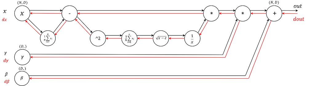
Some eye candy: a computational graph of a Batch Norm layer with a forward pass (black) and backward pass (red). (borrowed from this post)
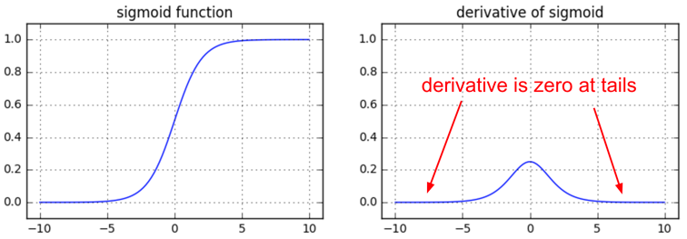
Vanishing gradients on sigmoids
We’re starting off easy here. At one point it was fashionable to use sigmoid (or tanh) non-linearities in the fully connected layers. The tricky part people might not realize until they think about the backward pass is that if you are sloppy with the weight initialization or data preprocessing these non-linearities can “saturate” and entirely stop learning — your training loss will be flat and refuse to go down. For example, a fully connected layer with sigmoid non-linearity computes (using raw numpy):
z = 1/(1 + np.exp(-np.dot(W, x))) # forward pass
dx = np.dot(W.T, z*(1-z)) # backward pass: local gradient for x
dW = np.outer(z*(1-z), x) # backward pass: local gradient for W
If your weight matrix W is initialized too large, the output of the matrix multiply could have a very large range (e.g. numbers between -400 and 400), which will make all outputs in the vector z almost binary: either 1 or 0. But if that is the case, z*(1-z), which is local gradient of the sigmoid non-linearity, will in both cases become zero (“vanish”), making the gradient for both x and W be zero. The rest of the backward pass will come out all zero from this point on due to multiplication in the chain rule.
Another non-obvious fun fact about sigmoid is that its local gradient (z*(1-z)) achieves a maximum at 0.25, when z = 0.5. That means that every time the gradient signal flows through a sigmoid gate, its magnitude always diminishes by one quarter (or more). If you’re using basic SGD, this would make the lower layers of a network train much slower than the higher ones.
TLDR: if you’re using sigmoids or tanh non-linearities in your network and you understand backpropagation you should always be nervous about making sure that the initialization doesn’t cause them to be fully saturated. See a longer explanation in this CS231n lecture video.
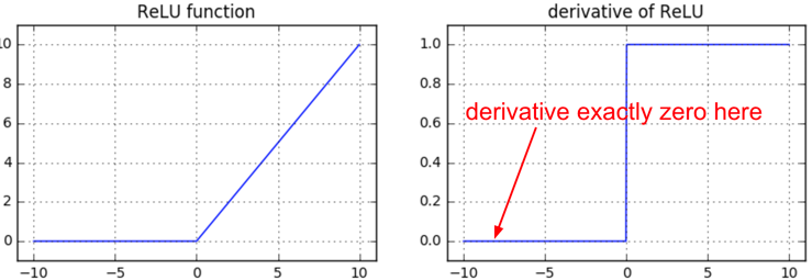
Dying ReLUs
Another fun non-linearity is the ReLU, which thresholds neurons at zero from below. The forward and backward pass for a fully connected layer that uses ReLU would at the core include:
z = np.maximum(0, np.dot(W, x)) # forward pass
dW = np.outer(z > 0, x) # backward pass: local gradient for W
If you stare at this for a while you’ll see that if a neuron gets clamped to zero in the forward pass (i.e. z=0, it doesn’t “fire”), then its weights will get zero gradient. This can lead to what is called the “dead ReLU” problem, where if a ReLU neuron is unfortunately initialized such that it never fires, or if a neuron’s weights ever get knocked off with a large update during training into this regime, then this neuron will remain permanently dead. It’s like permanent, irrecoverable brain damage. Sometimes you can forward the entire training set through a trained network and find that a large fraction (e.g. 40%) of your neurons were zero the entire time.
TLDR: If you understand backpropagation and your network has ReLUs, you’re always nervous about dead ReLUs. These are neurons that never turn on for any example in your entire training set, and will remain permanently dead. Neurons can also die during training, usually as a symptom of aggressive learning rates. See a longer explanation in CS231n lecture video.
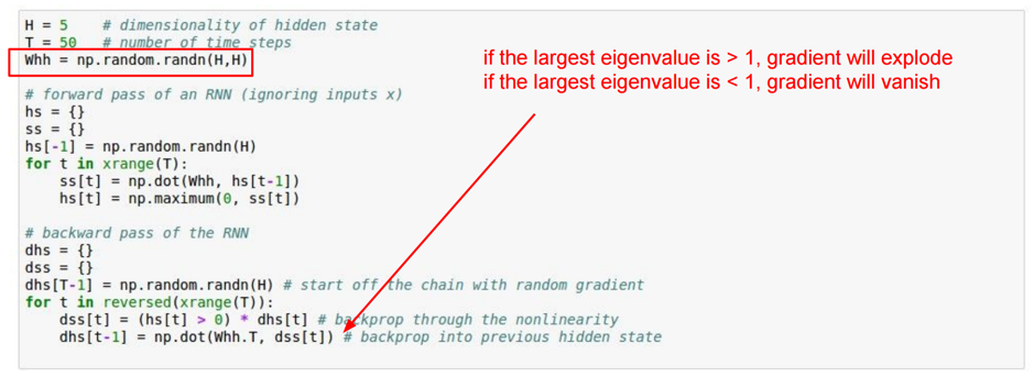
Exploding gradients in RNNs
Vanilla RNNs feature another good example of unintuitive effects of backpropagation. I’ll copy paste a slide from CS231n that has a simplified RNN that does not take any input x, and only computes the recurrence on the hidden state (equivalently, the input x could always be zero):
This RNN is unrolled for T time steps. When you stare at what the backward pass is doing, you’ll see that the gradient signal going backwards in time through all the hidden states is always being multiplied by the same matrix (the recurrence matrix Whh), interspersed with non-linearity backprop.
What happens when you take one number a and start multiplying it by some other number b (i.e. a*b*b*b*b*b*b…)? This sequence either goes to zero if |b| < 1, or explodes to infinity when |b|>1. The same thing happens in the backward pass of an RNN, except b is a matrix and not just a number, so we have to reason about its largest eigenvalue instead.
TLDR: If you understand backpropagation and you’re using RNNs you are nervous about having to do gradient clipping, or you prefer to use an LSTM. See a longer explanation in this CS231n lecture video.
Spotted in the Wild: DQN Clipping
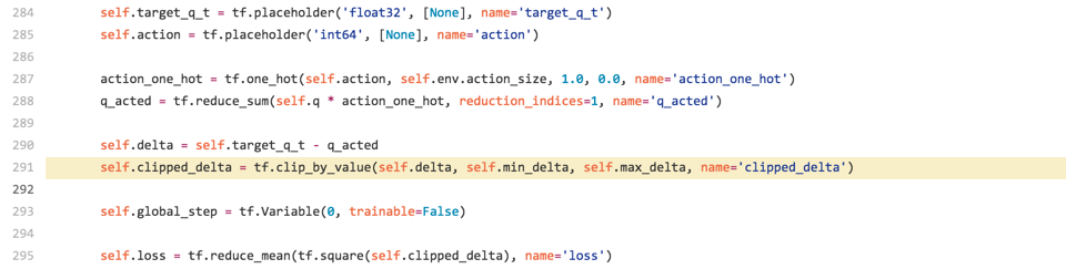
Lets look at one more — the one that actually inspired this post. Yesterday I was browsing for a Deep Q Learning implementation in TensorFlow (to see how others deal with computing the numpy equivalent of Q[:, a], where a is an integer vector — turns out this trivial operation is not supported in TF). Anyway, I searched “dqn tensorflow”, clicked the first link, and found the core code. Here is an excerpt:
If you’re familiar with DQN, you can see that there is the target_q_t, which is just [reward * gamma argmax_a Q(s’,a)], and then there is q_acted, which is Q(s,a) of the action that was taken. The authors here subtract the two into variable delta, which they then want to minimize on line 295 with the L2 loss with tf.reduce_mean(tf.square()). So far so good.
The problem is on line 291. The authors are trying to be robust to outliers, so if the delta is too large, they clip it with tf.clip_by_value. This is well-intentioned and looks sensible from the perspective of the forward pass, but it introduces a major bug if you think about the backward pass.
The clip_by_value function has a local gradient of zero outside of the range min_delta to max_delta, so whenever the delta is above min/max_delta, the gradient becomes exactly zero during backprop. The authors are clipping the raw Q delta, when they are likely trying to clip the gradient for added robustness. In that case the correct thing to do is to use the Huber loss in place of tf.square:
It’s a bit gross in TensorFlow because all we want to do is clip the gradient if it is above a threshold, but since we can’t meddle with the gradients directly we have to do it in this round-about way of defining the Huber loss. In Torch this would be much more simple.
I submitted an issue on the DQN repo and this was promptly fixed.
In conclusion
Backpropagation is a leaky abstraction; it is a credit assignment scheme with non-trivial consequences. If you try to ignore how it works under the hood because “TensorFlow automagically makes my networks learn”, you will not be ready to wrestle with the dangers it presents, and you will be much less effective at building and debugging neural networks.
The good news is that backpropagation is not that difficult to understand, if presented properly. I have relatively strong feelings on this topic because it seems to me that 95% of backpropagation materials out there present it all wrong, filling pages with mechanical math. Instead, I would recommend the CS231n lecture on backprop which emphasizes intuition (yay for shameless self-advertising). And if you can spare the time, as a bonus, work through the CS231n assignments, which get you to write backprop manually and help you solidify your understanding.
That’s it for now! I hope you’ll be much more suspicious of backpropagation going forward and think carefully through what the backward pass is doing. Also, I’m aware that this post has (unintentionally!) turned into several CS231n ads. Apologies for that 🙂


 We focus on applying tech to product. Thanks in great part to the open-source movement, it’s easier than ever to build a technology company. However, AI & ML innovation is still in its nascent phase and very hard to apply in the building of comprehensive solutions and scalable products.