Yes you should understand backprop
When we offered CS231n (Deep Learning class) at Stanford, we intentionally designed the programming assignments to include explicit calculations involved in backpropagation on the lowest level. The students had to implement the forward and the backward pass of each layer in raw numpy. Inevitably, some students complained on the class message boards:
“Why do we have to write the backward pass when frameworks in the real world, such as TensorFlow, compute them for you automatically?”
This is seemingly a perfectly sensible appeal – if you’re never going to write backward passes once the class is over, why practice writing them? Are we just torturing the students for our own amusement? Some easy answers could make arguments along the lines of “it’s worth knowing what’s under the hood as an intellectual curiosity”, or perhaps “you might want to improve on the core algorithm later”, but there is a much stronger and practical argument, which I wanted to devote a whole post to:
> The problem with Backpropagation is that it is a leaky abstraction.
In other words, it is easy to fall into the trap of abstracting away the learning process — believing that you can simply stack arbitrary layers together and backprop will “magically make them work” on your data. So lets look at a few explicit examples where this is not the case in quite unintuitive ways.
Vanishing gradients on sigmoids
We’re starting off easy here. At one point it was fashionable to use sigmoid (or tanh) non-linearities in the fully connected layers. The tricky part people might not realize until they think about the backward pass is that if you are sloppy with the weight initialization or data preprocessing these non-linearities can “saturate” and entirely stop learning — your training loss will be flat and refuse to go down. For example, a fully connected layer with sigmoid non-linearity computes (using raw numpy):
z = 1/(1 + np.exp(-np.dot(W, x))) # forward pass
dx = np.dot(W.T, z*(1-z)) # backward pass: local gradient for x
dW = np.outer(z*(1-z), x) # backward pass: local gradient for W
If your weight matrix W is initialized too large, the output of the matrix multiply could have a very large range (e.g. numbers between -400 and 400), which will make all outputs in the vector z almost binary: either 1 or 0. But if that is the case, z*(1-z), which is local gradient of the sigmoid non-linearity, will in both cases become zero (“vanish”), making the gradient for both x and W be zero. The rest of the backward pass will come out all zero from this point on due to multiplication in the chain rule.
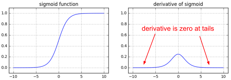
Another non-obvious fun fact about sigmoid is that its local gradient (z*(1-z)) achieves a maximum at 0.25, when z = 0.5. That means that every time the gradient signal flows through a sigmoid gate, its magnitude always diminishes by one quarter (or more). If you’re using basic SGD, this would make the lower layers of a network train much slower than the higher ones.
TLDR: if you’re using sigmoids or tanh non-linearities in your network and you understand backpropagation you should always be nervous about making sure that the initialization doesn’t cause them to be fully saturated. See a longer explanation in this CS231n lecture video.
Dying ReLUs
Another fun non-linearity is the ReLU, which thresholds neurons at zero from below. The forward and backward pass for a fully connected layer that uses ReLU would at the core include:
z = np.maximum(0, np.dot(W, x)) # forward pass
dW = np.outer(z > 0, x) # backward pass: local gradient for W
If you stare at this for a while you’ll see that if a neuron gets clamped to zero in the forward pass (i.e. z=0, it doesn’t “fire”), then its weights will get zero gradient. This can lead to what is called the “dead ReLU” problem, where if a ReLU neuron is unfortunately initialized such that it never fires, or if a neuron’s weights ever get knocked off with a large update during training into this regime, then this neuron will remain permanently dead. It’s like permanent, irrecoverable brain damage. Sometimes you can forward the entire training set through a trained network and find that a large fraction (e.g. 40%) of your neurons were zero the entire time.
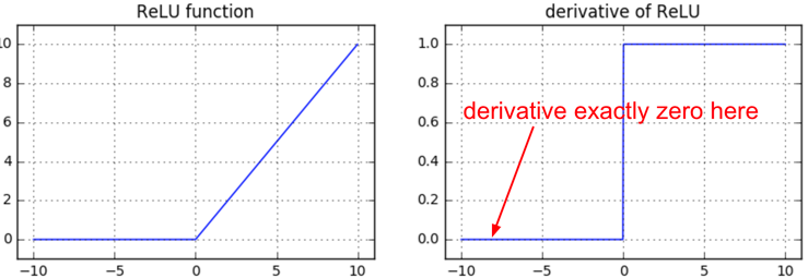
TLDR: If you understand backpropagation and your network has ReLUs, you’re always nervous about dead ReLUs. These are neurons that never turn on for any example in your entire training set, and will remain permanently dead. Neurons can also die during training, usually as a symptom of aggressive learning rates. See a longer explanation in CS231n lecture video.
Exploding gradients in RNNs
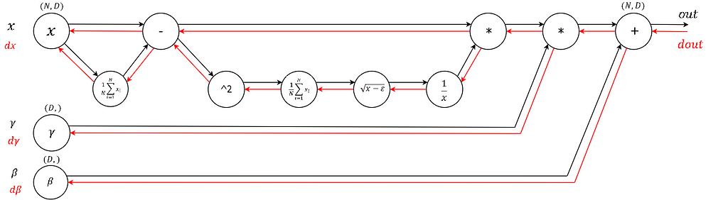
Vanilla RNNs feature another good example of unintuitive effects of backpropagation. I’ll copy paste a slide from CS231n that has a simplified RNN that does not take any input x, and only computes the recurrence on the hidden state (equivalently, the input x could always be zero):
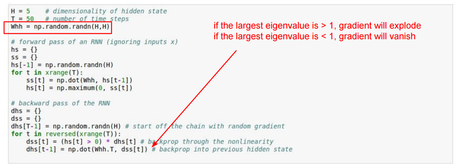
This RNN is unrolled for T time steps. When you stare at what the backward pass is doing, you’ll see that the gradient signal going backwards in time through all the hidden states is always being multiplied by the same matrix (the recurrence matrix Whh), interspersed with non-linearity backprop.
What happens when you take one number a and start multiplying it by some other number b (i.e. a*b*b*b*b*b*b…)? This sequence either goes to zero if |b| < 1, or explodes to infinity when |b|>1. The same thing happens in the backward pass of an RNN, except b is a matrix and not just a number, so we have to reason about its largest eigenvalue instead.
TLDR: If you understand backpropagation and you’re using RNNs you are nervous about having to do gradient clipping, or you prefer to use an LSTM. See a longer explanation in this CS231n lecture video.
Spotted in the Wild: DQN Clipping
Lets look at one more — the one that actually inspired this post. Yesterday I was browsing for a Deep Q Learning implementation in TensorFlow (to see how others deal with computing the numpy equivalent of Q[:, a], where a is an integer vector — turns out this trivial operation is not supported in TF). Anyway, I searched “dqn tensorflow”, clicked the first link, and found the core code. Here is an excerpt:
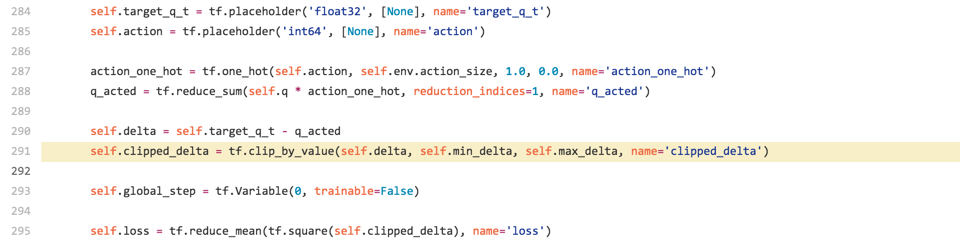
If you’re familiar with DQN, you can see that there is the target_q_t, which is just [reward * gamma argmax_a Q(s’,a)], and then there is q_acted, which is Q(s,a) of the action that was taken. The authors here subtract the two into variable delta, which they then want to minimize on line 295 with the L2 loss with tf.reduce_mean(tf.square()). So far so good.
The problem is on line 291. The authors are trying to be robust to outliers, so if the delta is too large, they clip it with tf.clip_by_value. This is well-intentioned and looks sensible from the perspective of the forward pass, but it introduces a major bug if you think about the backward pass.
The clip_by_value function has a local gradient of zero outside of the range min_delta to max_delta, so whenever the delta is above min/max_delta, the gradient becomes exactly zero during backprop. The authors are clipping the raw Q delta, when they are likely trying to clip the gradient for added robustness. In that case the correct thing to do is to use the Huber loss in place of tf.square:
def clipped_error(x):
  return tf.select(tf.abs(x) < 1.0,
                   0.5 * tf.square(x),
                   tf.abs(x) - 0.5) # condition, true, false
It’s a bit gross in TensorFlow because all we want to do is clip the gradient if it is above a threshold, but since we can’t meddle with the gradients directly we have to do it in this round-about way of defining the Huber loss. In Torch this would be much more simple.
I submitted an issue on the DQN repo and this was promptly fixed.
In conclusion
Backpropagation is a leaky abstraction; it is a credit assignment scheme with non-trivial consequences. If you try to ignore how it works under the hood because “TensorFlow automagically makes my networks learn”, you will not be ready to wrestle with the dangers it presents, and you will be much less effective at building and debugging neural networks.
The good news is that backpropagation is not that difficult to understand, if presented properly. I have relatively strong feelings on this topic because it seems to me that 95% of backpropagation materials out there present it all wrong, filling pages with mechanical math. Instead, I would recommend the CS231n lecture on backprop which emphasizes intuition (yay for shameless self-advertising). And if you can spare the time, as a bonus, work through the CS231n assignments, which get you to write backprop manually and help you solidify your understanding.
That’s it for now! I hope you’ll be much more suspicious of backpropagation going forward and think carefully through what the backward pass is doing. Also, I’m aware that this post has (unintentionally!) turned into several CS231n ads. Apologies for that 🙂