Word order and syntactic structure have a large impact on sentence meaning — even small perturbations in word order can completely change interpretation. For example, consider the following related sentences:

1. Flights from New York to Florida.
2. Flights to Florida from New York.
3. Flights from Florida to New York.

All three have the same set of words. However, 1 and 2 have the same meaning — known as paraphrase pairs — while 1 and 3 have very different meanings — known as non-paraphrase pairs. The task of identifying whether pairs are paraphrase or not is called paraphrase identification, and this task is important to many real-world natural language understanding (NLU) applications such as question answering. Perhaps surprisingly, even state-of-the-art models, like BERT, would fail to correctly identify the difference between many non-paraphrase pairs like 1 and 3 above if trained only on existing NLU datasets. This is because existing datasets lack training pairs like this, so it is hard for machine learning models to learn this pattern even if they have the capability to understand complex contextual phrasings.

To address this, we are releasing two new datasets for use in the research community: Paraphrase Adversaries from Word Scrambling (PAWS) in English, and PAWS-X, an extension of the PAWS dataset to six typologically distinct languages: French, Spanish, German, Chinese, Japanese, and Korean. Both datasets contain well-formed sentence pairs with high lexical overlap, in which about half of the pairs are paraphrase and others are not. Including new pairs in training data for state-of-the-art models improves their accuracy on this problem from <50% to 85-90%. In contrast, models that do not capture non-local contextual information fail even with new training examples. The new datasets therefore provide an effective instrument for measuring the sensitivity of models to word order and structure.

The PAWS dataset contains 108,463 human-labeled pairs in English, sourced from Quora Question Pairs (QQP) and Wikipedia pages. PAWS-X contains 23,659 human translated PAWS evaluation pairs and 296,406 machine translated training pairs. The table below gives detailed statistics of the datasets.

Creating the PAWS Dataset in English
In “PAWS: Paraphrase Adversaries from Word Scrambling,” we introduce a workflow for generating pairs of sentences that have high word overlap, but which are balanced with respect to whether they are paraphrases or not. To generate examples, source sentences are first passed to a specialized language model that creates word-swapped variants that are still semantically meaningful, but ambiguous as to whether they are paraphrase pairs or not. These were then judged by human raters for grammaticality and then multiple raters judged whether they were paraphrases of each other. 

PAWS corpus creation workflow.

One problem with this swapping strategy is that it tends to produce pairs that aren’t paraphrases (e.g., “why do bad things happen to good people” != “why do good things happen to bad people“). In order to ensure balance between paraphrases and non-paraphrases, we added other examples based on back-translation. Back-translation has the opposite bias as it tends to preserve meaning while changing word order and word choice. These two strategies lead to PAWS being balanced overall, especially for the Wikipedia portion.

Creating the Multilingual PAWS-X Dataset
After creating PAWS, we extended it to six more languages: Chinese, French, German, Korean, Japanese, and Spanish. We hired human translators to translate the development and test sets, and used a neural machine translation (NMT) service to translate the training set.
We obtained human translations (native speakers) on a random sample of 4,000 sentence pairs from the PAWS development set for each of the six languages (48,000 translations). Each sentence in a pair is presented independently so that translation is not affected by context. A randomly sampled subset was validated by a second worker. The final dataset has less than 5% word level error rate.
Note, we allowed professionals to not translate a sentence if it was incomplete or ambiguous. On average, less than 2% of the pairs were not translated, and we simply excluded them. The final translated pairs are split then into new development and test sets, ~2,000 pairs for each.

Examples of human translated pairs for German(de) and Chinese(zh).

Language Understanding with PAWS and PAWS-X
We train multiple models on the created dataset and measure the classification accuracy on the eval set. When trained with PAWS, strong models, such as BERT and DIIN, show remarkable improvement over when they are trained on the existing Quora Question Pairs (QQP) dataset. For example, on the PAWS data sourced from QQP (PAWS-QQP), BERT gets only 33.5 accuracy if trained on existing QQP, but it recovers to 83.1 accuracy when given PAWS training examples. Unlike BERT, a simple Bag-of-Words (BOW) model fails to learn from PAWS training examples, demonstrating its weakness at capturing non-local contextual information. These results demonstrate that PAWS effectively measures sensitivity of models to word order and structure.

Accuracy on PAWS-QQP Eval Set (English).

The figure below shows the performance of the popular multilingual BERT model on PAWS-X using several common strategies:

1. Zero Shot: The model is trained on the PAWS English training data, and then directly evaluated on all others. Machine translation is not involved in this strategy.
2. Translate Test: Train a model using the English training data, and machine-translate all test examples to English for evaluation.
3. Translate Train: The English training data is machine-translated into each target language to provide data to train each model.
4. Merged: Train a multilingual model on all languages, including the original English pairs and machine-translated data in all other languages.

The results show that cross-lingual techniques help, while it also leaves considerable headroom to drive multilingual research on the problem of paraphrase identification

Accuracy of PAWS-X Test Set using BERT Models.

It is our hope that these datasets will be useful to the research community to drive further progress on multilingual models that better exploit structure, context, and pairwise comparisons.

Acknowledgements
The core team includes Luheng He, Jason Baldridge, Chris Tar. We would like to thank the Language team in Google Research, especially Emily Pitler, for the insightful comments that contributed to our papers. Many thanks also to Ashwin Kakarla, Henry Jicha, and Mengmeng Niu, for the help with the annotations.

Google’s mission is not just to organize the world’s information but to make it universally accessible, which means ensuring that our products work in as many of the world’s languages as possible. When it comes to understanding human speech, which is a core capability of the Google Assistant, extending to more languages poses a challenge: high-quality automatic speech recognition (ASR) systems require large amounts of audio and text data — even more so as data-hungry neural models continue to revolutionize the field. Yet many languages have little data available.

We wondered how we could keep the quality of speech recognition high for speakers of data-scarce languages. A key insight from the research community was that much of the “knowledge” a neural network learns from audio data of a data-rich language is re-usable by data-scarce languages; we don’t need to learn everything from scratch. This led us to study multilingual speech recognition, in which a single model learns to transcribe multiple languages.

In “Large-Scale Multilingual Speech Recognition with a Streaming End-to-End Model”, published at Interspeech 2019, we present an end-to-end (E2E) system trained as a single model, which allows for real-time multilingual speech recognition. Using nine Indian languages, we demonstrated a dramatic improvement in the ASR quality on several data-scarce languages, while still improving performance for the data-rich languages.

India: A Land of Languages
For this study, we focused on India, an inherently multilingual society where there are more than thirty languages with at least a million native speakers. Many of these languages overlap in acoustic and lexical content due to the geographic proximity of the native speakers and shared cultural history. Additionally, many Indians are bilingual or trilingual, making the use of multiple languages within a conversation a common phenomenon, and a natural case for training a single multilingual model. In this work, we combined nine primary Indian languages, namely Hindi, Marathi, Urdu, Bengali, Tamil, Telugu, Kannada, Malayalam and Gujarati.

A Low-latency All-neural Multilingual Model
Traditional ASR systems contain separate components for acoustic, pronunciation, and language models. While there have been attempts to make some or all of the traditional ASR components multilingual [1,2,3,4], this approach can be complex and difficult to scale. E2E ASR models combine all three components into a single neural network and promise scalability and ease of parameter sharing. Recent works have extended E2E models to be multilingual [1,2], but they did not address the need for real-time speech recognition, a key requirement for applications such as the Assistant, Voice Search and GBoard dictation. For this, we turned to recent research at Google that used a Recurrent Neural Network Transducer (RNN-T) model to achieve streaming E2E ASR. The RNN-T system outputs words one character at a time, just as if someone was typing in real time, however this was not multilingual. We built upon this architecture to develop a low-latency model for multilingual speech recognition.

[Left] A traditional monolingual speech recognizer comprising of Acoustic, Pronunciation and Language Models for each language. [Middle] A traditional multilingual speech recognizer where the Acoustic and Pronunciation model is multilingual, while the Language model is language-specific. [Right] An E2E multilingual speech recognizer where the Acoustic, Pronunciation and Language Model is combined into a single multilingual model.

Large-Scale Data Challenges
Using large-scale, real-world data for training a multilingual model is complicated by data imbalance. Given the steep skew in the distribution of speakers across the languages and speech product maturity, it is not surprising to have varying amounts of transcribed data available per language. As a result, a multilingual model can tend to be more influenced by languages that are over-represented in the training set. This bias is more prominent in an E2E model, which unlike a traditional ASR system, does not have access to additional in-language text data and learns lexical characteristics of the languages solely from the audio training data.

Histogram of training data for the nine languages showing the steep skew in the data available.

We addressed this issue with a few architectural modifications. First, we provided an extra language identifier input, which is an external signal derived from the language locale of the training data; i.e. the language preference set in an individual’s phone. This signal is combined with the audio input as a one-hot feature vector. We hypothesize that the model is able to use the language vector not only to disambiguate the language but also to learn separate features for separate languages, as needed, which helped with data imbalance.

Building on the idea of language-specific representations within the global model, we further augmented the network architecture by allocating extra parameters per language in the form of residual adapter modules. Adapters helped fine-tune a global model on each language while maintaining parameter efficiency of a single global model, and in turn, improved performance.

[Left] Multilingual RNN-T architecture with a language identifier. [Middle] Residual adapters inside the encoder. For a Tamil utterance, only the Tamil adapters are applied to each activation. [Right] Architecture details of the Residual Adapter modules. For more details please see our paper.

Putting all of these elements together, our multilingual model outperforms all the single-language recognizers, with especially large improvements in data-scarce languages like Kannada and Urdu. Moreover, since it is a streaming E2E model, it simplifies training and serving, and is also usable in low-latency applications like the Assistant. Building on this result, we hope to continue our research on multilingual ASRs for other language groups, to better assist our growing body of diverse users.

Acknowledgements
We would like to thank the following for their contribution to this research: Tara N. Sainath, Eugene Weinstein, Bo Li, Shubham Toshniwal, Ron Weiss, Bhuvana Ramabhadran, Yonghui Wu, Ankur Bapna, Zhifeng Chen, Seungji Lee, Meysam Bastani, Mikaela Grace, Pedro Moreno, Yanzhang (Ryan) He, Khe Chai Sim.

Deep learning has given rise to technologies that would have been thought impossible only a handful of years ago. Modern generative models are one example of these, capable of synthesizing hyperrealistic images, speech, music, and even video. These models have found use in a wide variety of applications, including making the world more accessible through text-to-speech, and helping generate training data for medical imaging.

Like any transformative technology, this has created new challenges. So-called “deepfakes“—produced by deep generative models that can manipulate video and audio clips—are one of these. Since their first appearance in late 2017, many open-source deepfake generation methods have emerged, leading to a growing number of synthesized media clips. While many are likely intended to be humorous, others could be harmful to individuals and society.

Google considers these issues seriously. As we published in our AI Principles last year, we are committed to developing AI best practices to mitigate the potential for harm and abuse. Last January, we announced our release of a dataset of synthetic speech in support of an international challenge to develop high-performance fake audio detectors. The dataset was downloaded by more than 150 research and industry organizations as part of the challenge, and is now freely available to the public.

Today, in collaboration with Jigsaw, we’re announcing the release of a large dataset of visual deepfakes we’ve produced that has been incorporated into the Technical University of Munich and the University Federico II of Naples’ new FaceForensics benchmark, an effort that Google co-sponsors. The incorporation of these data into the FaceForensics video benchmark is in partnership with leading researchers, including Prof. Matthias Niessner, Prof. Luisa Verdoliva and the FaceForensics team. You can download the data on the FaceForensics github page.

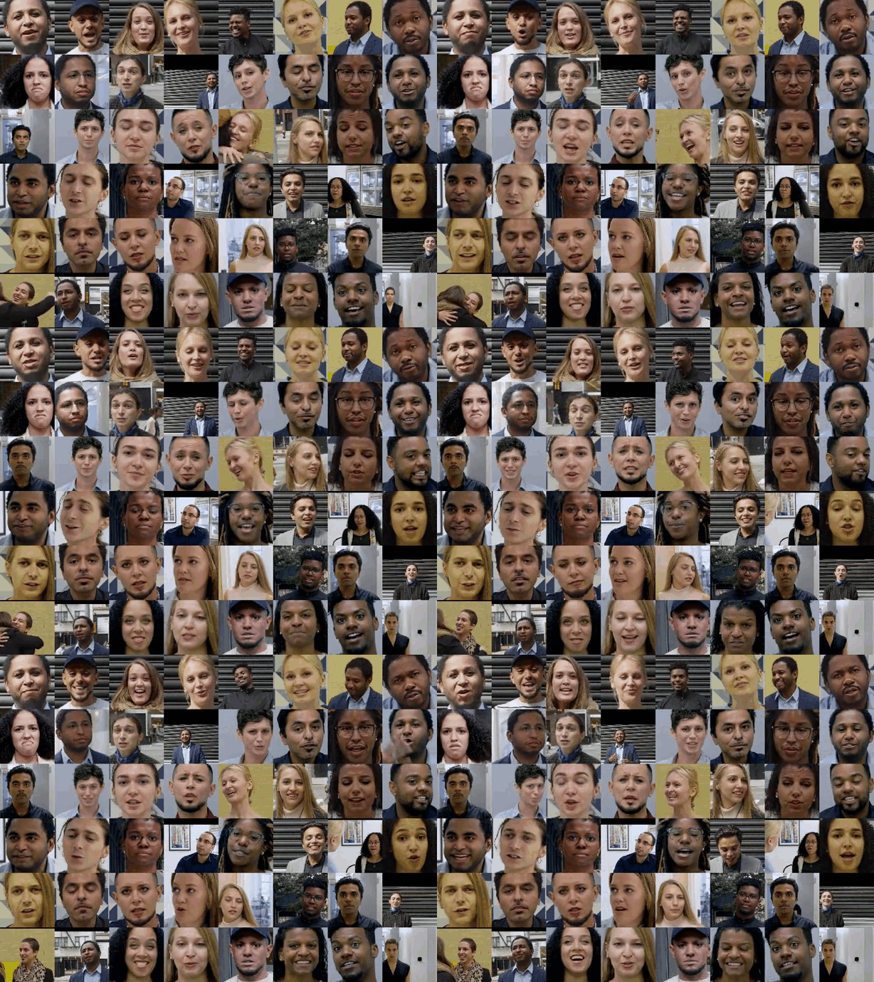
A sample of videos from Google’s contribution to the FaceForensics benchmark. To generate these, pairs of actors were selected randomly and deep neural networks swapped the face of one actor onto the head of another.

To make this dataset, over the past year we worked with paid and consenting actors to record hundreds of videos. Using publicly available deepfake generation methods, we then created thousands of deepfakes from these videos. The resulting videos, real and fake, comprise our contribution, which we created to directly support deepfake detection efforts. As part of the FaceForensics benchmark, this dataset is now available, free to the research community, for use in developing synthetic video detection methods.

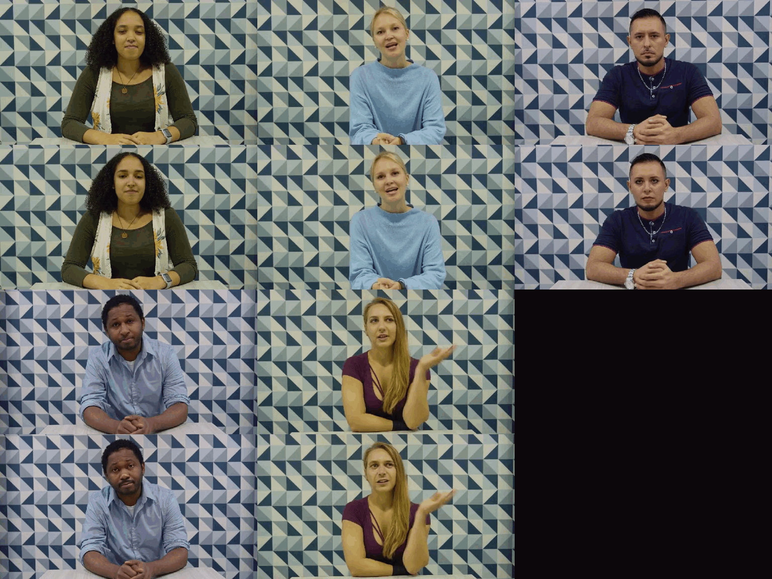
Actors were filmed in a variety of scenes. Some of these actors are pictured here (top) with an example deepfake (bottom), which can be a subtle or drastic change, depending on the other actor used to create them.

Since the field is moving quickly, we’ll add to this dataset as deepfake technology evolves over time, and we’ll continue to work with partners in this space. We firmly believe in supporting a thriving research community around mitigating potential harms from misuses of synthetic media, and today’s release of our deepfake dataset in the FaceForensics benchmark is an important step in that direction.

Acknowledgements
Special thanks to all our team members and collaborators who work on this project with us: Daisy Stanton, Per Karlsson, Alexey Victor Vorobyov, Thomas Leung, Jeremiah “Spudde” Childs, Christoph Bregler, Andreas Roessler, Davide Cozzolino, Justus Thies, Luisa Verdoliva, Matthias Niessner, and the hard-working actors and film crew who helped make this dataset possible.

Several years ago, we identified flood forecasts as a unique opportunity to improve people’s lives, and began looking into how Google’s infrastructure and machine learning expertise can help in this field. Last year, we started our flood forecasting pilot in the Patna region, and since then we have expanded our flood forecasting coverage, as part of our larger AI for Social Good efforts. In this post, we discuss some of the technology and methodology behind this effort.

The Inundation Model
A critical step in developing an accurate flood forecasting system is to develop inundation models, which use either a measurement or a forecast of the water level in a river as an input, and simulate the water behavior across the floodplain.

A 3D visualization of a hydraulic model simulating various river conditions.

This allows us to translate current or future river conditions, to highly spatially accurate risk maps – which tell us what areas will be flooded and what areas will be safe. Inundation models depend on four major components, each with its own challenges and innovations:

Real-time Water Level Measurements
To run these models operationally, we need to know what is happening on the ground in real-time, and thus we rely on partnerships with the relevant government agencies to receive timely and accurate information. Our first governmental partner is the Indian Central Water Commission (CWC), which measures water levels hourly in over a thousand stream gauges across all of India, aggregates this data, and produces forecasts based on upstream measurements. The CWC provides these real-time river measurements and forecasts, which are then used as inputs for our models.

CWC employees measuring water level and discharge near Lucknow, India.

Elevation Map Creation
Once we know how much water is in a river, it is critical that the models have a good map of the terrain. High-resolution digital elevation models (DEMs) are incredibly useful for a wide range of applications in the earth sciences, but are still difficult to acquire in most of the world, especially for flood forecasting. This is because meter-wide features of the ground conditions can create a critical difference in the resulting flooding (embankments are one exceptionally important example), but publicly accessible global DEMs have resolutions of tens of meters. To help address this challenge, we’ve developed a novel methodology to produce high resolution DEMs based on completely standard optical imagery.

We start with the large and varied collection of satellite images used in Google Maps. Correlating and aligning the images in large batches, we simultaneously optimize for satellite camera model corrections (for orientation errors, etc.) and for coarse terrain elevation. We then use the corrected camera models to create a depth map for each image. To make the elevation map, we optimally fuse the depth maps together at each location. Finally, we remove objects such as trees and bridges so that they don’t block water flow in our simulations. This can be done manually or by training convolutional neural networks that can identify where the terrain elevations need to be interpolated. The result is a roughly 1 meter DEM, which can be used to run hydraulic models.

Hydraulic Modeling
Once we have both these inputs – the riverine measurements and forecasts, and the elevation map – we can begin the modeling itself, which can be divided into two main components. The first and most substantial component is the physics-based hydraulic model, which updates the location and velocity of the water through time based on (an approximated) computation of the laws of physics. Specifically, we’ve implemented a solver for the 2D form of the shallow-water Saint-Venant equations. These models are suitably accurate when given accurate inputs and run at high resolutions, but their computational complexity creates challenges – it is proportional to the cube of the resolution desired. That is, if you double the resolution, you’ll need roughly 8 times as much processing time. Since we’re committed to the high-resolution required for highly accurate forecasts, this can lead to unscalable computational costs, even for Google!

To help address this problem, we’ve created a unique implementation of our hydraulic model, optimized for Tensor Processing Units (TPUs). While TPUs were optimized for neural networks (rather than differential equation solvers like our hydraulic model), their highly parallelized nature leads to the performance per TPU core being 85x times faster than the performance per CPU core. For additional efficiency improvements, we’re also looking at using machine learning to replace some of the physics-based algorithmics, extending data-driven discretization to two-dimensional hydraulic models, so we can support even larger grids and cover even more people.

A snapshot of a TPU-based simulation of flooding in Goalpara, mid-event.

As mentioned earlier, the hydraulic model is only one component of our inundation forecasts. We’ve repeatedly found locations where our hydraulic models are not sufficiently accurate – whether that’s due to inaccuracies in the DEM, breaches in embankments, or unexpected water sources. Our goal is to find effective ways to reduce these errors. For this purpose, we added a predictive inundation model, based on historical measurements. Since 2014, the European Space Agency has been operating a satellite constellation named Sentinel-1 with C-band Synthetic-Aperture Radar (SAR) instruments. SAR imagery is great at identifying inundation, and can do so regardless of weather conditions and clouds. Based on this valuable data set, we correlate historical water level measurements with historical inundations, allowing us to identify consistent corrections to our hydraulic model. Based on the outputs of both components, we can estimate which disagreements are due to genuine ground condition changes, and which are due to modeling inaccuracies.

Flood warnings across Google’s interfaces.

Looking Forward
We still have a lot to do to fully realize the benefits of our inundation models. First and foremost, we’re working hard to expand the coverage of our operational systems, both within India and to new countries. There’s also a lot more information we want to be able to provide in real time, including forecasted flood depth, temporal information and more. Additionally, we’re researching how to best convey this information to individuals to maximize clarity and encourage them to take the necessary protective actions.

Computationally, while the inundation model is a good tool for improving the spatial resolution (and therefore the accuracy and reliability) of existing flood forecasts, multiple governmental agencies and international organizations we’ve spoken to are concerned about areas that do not have access to effective flood forecasts at all, or whose forecasts don’t provide enough lead time for effective response. In parallel to our work on the inundation model, we’re working on some basic research into improved hydrologic models, which we hope will allow governments not only to produce more spatially accurate forecasts, but also achieve longer preparation time.

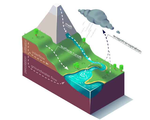
Hydrologic models accept as inputs things like precipitation, solar radiation, soil moisture and the like, and produce a forecast for the river discharge (among other things), days into the future. These models are traditionally implemented using a combination of conceptual models approximating different core processes such as snowmelt, surface runoff, evapotranspiration and more.

The core processes of a hydrologic model. Designed by Daniel Klotz, JKU Institute for Machine Learning.

These models also traditionally require a large amount of manual calibration, and tend to underperform in data scarce regions. We are exploring how multi-task learning can be used to address both of these problems — making hydrologic models both more scalable, and more accurate. In research collaboration with JKU Institute For Machine Learning group under Sepp Hochreiter on developing ML-based hydrologic models, Kratzert et al. show how LSTMs perform better than all benchmarked classic hydrologic models.

The distribution of NSE scores on basins across the United States for various models, showing the proposed EA-LSTM consistently outperforming a wide range of commonly used models.

Though this work is still in the basic research stage and not yet operational, we think it is an important first step, and hope it can already be useful for other researchers and hydrologists. It’s an incredible privilege to take part in the large eco-system of researchers, governments, and NGOs working to reduce the harms of flooding. We’re excited about the potential impact this type of research can provide, and look forward to where research in this field will go.

Acknowledgements
There are many people who contributed to this large effort, and we’d like to highlight some of the key contributors: Aaron Yonas, Adi Mano, Ajai Tirumali, Avinatan Hassidim, Carla Bromberg, Damien Pierce, Gal Elidan, Guy Shalev, John Anderson, Karan Agarwal, Kartik Murthy, Manan Singhi, Mor Schlesinger, Ofir Reich, Oleg Zlydenko, Pete Giencke, Piyush Poddar, Ruha Devanesan, Slava Salasin, Varun Gulshan, Vova Anisimov, Yossi Matias, Yi-fan Chen, Yotam Gigi, Yusef Shafi, Zach Moshe and Zvika Ben-Haim.

The discoveries being made regularly in neuroscience are an ongoing source of inspiration for creating more efficient artificial neural networks that process information in the same way as biological organisms. These networks have recently achieved resounding success in domains ranging from playing board and video games to fine-grained understanding of video. However, there is one fundamental aspect of biological brains that artificial neural networks are not yet fully leveraging: temporal encoding of information. Preserving temporal information allows a better representation of dynamic features, such as sounds, and enables fast responses to events that may occur at any moment. Furthermore, despite the fact that biological systems can consist of billions of neurons, information can be carried by a single signal (‘spike’) fired by an individual neuron, with information encoded in the timing of the signal itself.

Based on this biological insight, project Ihmehimmeli explores how artificial spiking neural networks can exploit temporal dynamics using various architectures and learning settings. “Ihmehimmeli” is a Finnish tongue-in-cheek word for a complex tool or a machine element whose purpose is not immediately easy to grasp. The essence of this word captures our aim to build complex recurrent neural network architectures with temporal encoding of information. We use artificial spiking networks with a temporal coding scheme, in which more interesting or surprising information, such as louder sounds or brighter colours, causes earlier neuronal spikes. Along the information processing hierarchy, the winning neurons are those that spike first. Such an encoding can naturally implement a classification scheme where input features are encoded in the spike times of their corresponding input neurons, while the output class is encoded by the output neuron that spikes earliest.

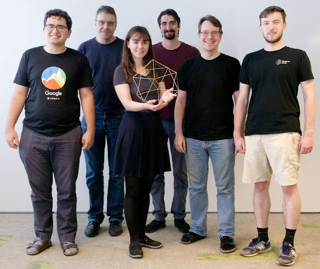
The Ihmehimmeli project team holding a himmeli, a symbol for the aim to build recurrent neural network architectures with temporal encoding of information.

We recently published and open-sourced a model in which we demonstrated the computational capabilities of fully connected spiking networks that operate using temporal coding. Our model uses a biologically-inspired synaptic transfer function, where the electric potential on the membrane of a neuron rises and gradually decays over time in response to an incoming signal, until there is a spike. The strength of the associated change is controlled by the “weight” of the connection, which represents the synapse efficiency. Crucially, this formulation allows exact derivatives of postsynaptic spike times with respect to presynaptic spike times and weights. The process of training the network consists of adjusting the weights between neurons, which in turn leads to adjusted spike times across the network. Much like in conventional artificial neural networks, this was done using backpropagation. We used synchronization pulses, whose timing is also learned with backpropagation, to provide a temporal reference to the network.

We trained the network on classic machine learning benchmarks, with features encoded in time. The spiking network successfully learned to solve noisy Boolean logic problems and achieved a test accuracy of 97.96% on MNIST, a result comparable to conventional fully connected networks with the same architecture. However, unlike conventional networks, our spiking network uses an encoding that is in general more biologically-plausible, and, for a small trade-off in accuracy, can compute the result in a highly energy-efficient manner, as detailed below.

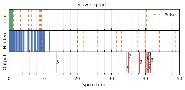
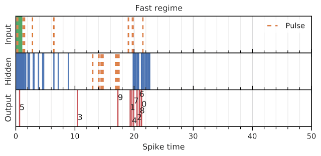
While training the spiking network on MNIST, we observed the neural network spontaneously shift between two operating regimes. Early during training, the network exhibited a slow and highly accurate regime, where almost all neurons fired before the network made a decision. Later in training, the network spontaneously shifted into a fast but slightly less accurate regime. This behaviour was intriguing, as we did not optimize for it explicitly. Thus spiking networks can, in a sense, be “deliberative”, or make a snap decision on the spot. This is reminiscent of the trade-off between speed and accuracy in human decision-making.

A slow (“deliberative”) network (top) and a fast (“impulsive”) network (bottom) classifying the same MNIST digit. The figures show a raster plot of spike times of individual neurons in individual layers, with synchronization pulses shown in orange. In this example, both networks classify the digit correctly; overall, the “slow” network achieves better accuracy than the “fast” network.

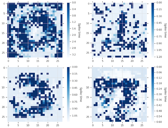
We were also able to recover representations of the digits learned by the spiking network by gradually adjusting a blank input image to maximize the response of a target output neuron. This indicates that the network learns human-like representations of the digits, as opposed to other possible combinations of pixels that might look “alien” to people. Having interpretable representations is important in order to understand what the network is truly learning and to prevent a small change in input from causing a large change in the result.

How the network “imagines” the digits 0, 1, 3 and 7.

This work is one example of an initial step that project Ihmehimmeli is taking in exploring the potential of time-based biology-inspired computing. In other on-going experiments, we are training spiking networks with temporal coding to control the walking of an artificial insect in a virtual environment, or taking inspiration from the development of the neural system to train a 2D spiking grid to predict words using axonal growth. Our goal is to increase our familiarity with the mechanisms that nature has evolved for natural intelligence, enabling the exploration of time-based artificial neural networks with varying internal states and state transitions.

Acknowledgements
The work described here was authored by Iulia Comsa, Krzysztof Potempa, Luca Versari, Thomas Fischbacher, Andrea Gesmundo and Jyrki Alakuijala. We are grateful for all discussions and feedback on this work that we received from our colleagues at Google.

This week, Graz, Austria hosts the 20th Annual Conference of the International Speech Communication Association (Interspeech 2019), one of the world‘s most extensive conferences on the research and engineering for spoken language processing. Over 2,000 experts in speech-related research fields gather to take part in oral presentations and poster sessions and to collaborate with streamed events across the globe.

As a Gold Sponsor of Interspeech 2019, we are excited to present 30 research publications, and demonstrate some of the impact speech technology has made in our products, from accessible, automatic video captioning to a more robust, reliable Google Assistant. If you’re attending Interspeech 2019, we hope that you’ll stop by the Google booth to meet our researchers and discuss projects and opportunities at Google that go into solving interesting problems for billions of people. Our researchers will also be on hand to discuss Google Cloud Text-to-Speech and Speech-to-text, demo Parrotron, and more. You can also learn more about the Google research being presented at Interspeech 2019 below (Google affiliations in blue).

Organizing Committee includes:
Michiel Bacchiani

Technical Program Committee includes:
Tara Sainath

Tutorials
Neural Machine Translation
Organizers include: Wolfgang Macherey, Yuan Cao

Accepted Publications
Building Large-Vocabulary ASR Systems for Languages Without Any Audio Training Data (link to appear soon)
Manasa Prasad, Daan van Esch, Sandy Ritchie, Jonas Fromseier Mortensen

Multi-Microphone Adaptive Noise Cancellation for Robust Hotword Detection (link to appear soon)
Yiteng Huang, Turaj Shabestary, Alexander Gruenstein, Li Wan

Direct Speech-to-Speech Translation with a Sequence-to-Sequence Model
Ye Jia, Ron Weiss, Fadi Biadsy, Wolfgang Macherey, Melvin Johnson, Zhifeng Chen, Yonghui Wu

Improving Keyword Spotting and Language Identification via Neural Architecture Search at Scale (link to appear soon)
Hanna Mazzawi, Javier Gonzalvo, Aleks Kracun, Prashant Sridhar, Niranjan Subrahmanya, Ignacio Lopez Moreno, Hyun Jin Park, Patrick Violette

Shallow-Fusion End-to-End Contextual Biasing (link to appear soon)
Ding Zhao, Tara Sainath, David Rybach, Pat Rondon, Deepti Bhatia, Bo Li, Ruoming Pang

VoiceFilter: Targeted Voice Separation by Speaker-Conditioned Spectrogram Masking
Quan Wang, Hannah Muckenhirn, Kevin Wilson, Prashant Sridhar, Zelin Wu, John Hershey, Rif Saurous, Ron Weiss, Ye Jia, Ignacio Lopez Moreno

SpecAugment: A Simple Data Augmentation Method for Automatic Speech Recognition
Daniel Park, William Chan, Yu Zhang, Chung-Cheng Chiu, Barret Zoph, Ekin Dogus Cubuk, Quoc Le

Two-Pass End-to-End Speech Recognition
Ruoming Pang, Tara Sainath, David Rybach, Yanzhang He, Rohit Prabhavalkar, Mirko Visontai, Qiao Liang, Trevor Strohman, Yonghui Wu, Ian McGraw, Chung-Cheng Chiu

On the Choice of Modeling Unit for Sequence-to-Sequence Speech Recognition
Kazuki Irie, Rohit Prabhavalkar, Anjuli Kannan, Antoine Bruguier, David Rybach, Patrick Nguyen

Contextual Recovery of Out-of-Lattice Named Entities in Automatic Speech Recognition (link to appear soon)
Jack Serrino, Leonid Velikovich, Petar Aleksic, Cyril Allauzen

Joint Speech Recognition and Speaker Diarization via Sequence Transduction
Laurent El Shafey, Hagen Soltau, Izhak Shafran

Personalizing ASR for Dysarthric and Accented Speech with Limited Data
Joel Shor, Dotan Emanuel, Oran Lang, Omry Tuval, Michael Brenner, Julie Cattiau, Fernando Vieira, Maeve McNally, Taylor Charbonneau, Melissa Nollstadt, Avinatan Hassidim, Yossi Matias

An Investigation Into On-Device Personalization of End-to-End Automatic Speech Recognition Models (link to appear soon)
Khe Chai Sim, Petr Zadrazil, Francoise Beaufays

Salient Speech Representations Based on Cloned Networks
Bastiaan Kleijn, Felicia Lim, Michael Chinen, Jan Skoglund

Cross-Lingual Consistency of Phonological Features: An Empirical Study (link to appear soon)
Cibu Johny, Alexander Gutkin, Martin Jansche

LibriTTS: A Corpus Derived from LibriSpeech for Text-to-Speech
Heiga Zen, Viet Dang, Robert Clark, Yu Zhang, Ron Weiss, Ye Jia, Zhifeng Chen, Yonghui Wu

Improving Performance of End-to-End ASR on Numeric Sequences
Cal Peyser, Hao Zhang, Tara Sainath, Zelin Wu

Developing Pronunciation Models in New Languages Faster by Exploiting Common Grapheme-to-Phoneme Correspondences Across Languages (link to appear soon)
Harry Bleyan, Sandy Ritchie, Jonas Fromseier Mortensen, Daan van Esch

Phoneme-Based Contextualization for Cross-Lingual Speech Recognition in End-to-End Models
Ke Hu, Antoine Bruguier, Tara Sainath, Rohit Prabhavalkar, Golan Pundak

Fréchet Audio Distance: A Reference-free Metric for Evaluating Music Enhancement Algorithms
Kevin Kilgour, Mauricio Zuluaga, Dominik Roblek, Matthew Sharifi

Learning to Speak Fluently in a Foreign Language: Multilingual Speech Synthesis and Cross-Language Voice Cloning
Yu Zhang, Ron Weiss, Heiga Zen, Yonghui Wu, Zhifeng Chen, RJ Skerry-Ryan, Ye Jia, Andrew Rosenberg, Bhuvana Ramabhadran

Sampling from Stochastic Finite Automata with Applications to CTC Decoding
Martin Jansche, Alexander Gutkin

Large-Scale Multilingual Speech Recognition with a Streaming End-to-End Model (link to appear soon)
Anjuli Kannan, Arindrima Datta, Tara Sainath, Eugene Weinstein, Bhuvana Ramabhadran, Yonghui Wu, Ankur Bapna, Zhifeng Chen, SeungJi Lee

A Real-Time Wideband Neural Vocoder at 1.6 kb/s Using LPCNet
Jean-Marc Valin, Jan Skoglund

Low-Dimensional Bottleneck Features for On-Device Continuous Speech Recognition
David Ramsay, Kevin Kilgour, Dominik Roblek, Matthew Sharif

Unified Verbalization for Speech Recognition & Synthesis Across Languages (link to appear soon)
Sandy Ritchie, Richard Sproat, Kyle Gorman, Daan van Esch, Christian Schallhart, Nikos Bampounis, Benoit Brard, Jonas Mortensen, Amelia Holt, Eoin Mahon

Better Morphology Prediction for Better Speech Systems (link to appear soon)
Dravyansh Sharma, Melissa Wilson, Antoine Bruguier

Dual Encoder Classifier Models as Constraints in Neural Text Normalization
Ajda Gokcen, Hao Zhang, Richard Sproat

Large-Scale Visual Speech Recognition
Brendan Shillingford, Yannis Assael, Matthew Hoffman, Thomas Paine, Cían Hughes, Utsav Prabhu, Hank Liao, Hasim Sak, Kanishka Rao, Lorrayne Bennett, Marie Mulville, Ben Coppin, Ben Laurie, Andrew Senior, Nando de Freitas

Parrotron: An End-to-End Speech-to-Speech Conversion Model and its Applications to Hearing-Impaired Speech and Speech Separation
Fadi Biadsy, Ron Weiss, Pedro Moreno, Dimitri Kanevsky, Ye Jia

An estimated 1.9 billion people worldwide suffer from a skin condition at any given time, and due to a shortage of dermatologists, many cases are seen by general practitioners instead. In the United States alone, up to 37% of patients seen in the clinic have at least one skin complaint and more than half of those patients are seen by non-dermatologists. However, studies demonstrate a significant gap in the accuracy of skin condition diagnoses between general practitioners and dermatologists, with the accuracy of general practitioners between 24% and 70%, compared to 77–96% for dermatologists. This can lead to suboptimal referrals, delays in care, and errors in diagnosis and treatment.

Existing strategies for non-dermatologists to improve diagnostic accuracy include the use of reference textbooks, online resources, and consultation with a colleague. Machine learning tools have also been developed with the aim of helping to improve diagnostic accuracy. Previous research has largely focused on early screening of skin cancer, in particular, whether a lesion is malignant or benign, or whether a lesion is melanoma. However, upwards of 90% of skin problems are not malignant, and addressing these more common conditions is also important to reduce the global burden of skin disease.

In “A Deep Learning System for Differential Diagnosis of Skin Diseases,” we developed a deep learning system (DLS) to address the most common skin conditions seen in primary care. Our results showed that a DLS can achieve an accuracy across 26 skin conditions that is on par with U.S. board-certified dermatologists, when presented with identical information about a patient case (images and metadata). This study highlights the potential of the DLS to augment the ability of general practitioners who did not have additional specialty training to accurately diagnose skin conditions.

DLS Design
Clinicians often face ambiguous cases for which there is no clear cut answer. For example, is this patient’s rash stasis dermatitis or cellulitis, or perhaps both superimposed? Rather than giving just one diagnosis, clinicians generate a differential diagnosis, which is a ranked list of possible diagnoses. A differential diagnosis frames the problem so that additional workup (laboratory tests, imaging, procedures, consultations) and treatments can be systematically applied until a diagnosis is confirmed. As such, a deep learning system (DLS) that produces a ranked list of possible skin conditions for a skin complaint closely mimics how clinicians think and is key to prompt triage, diagnosis and treatment for patients.

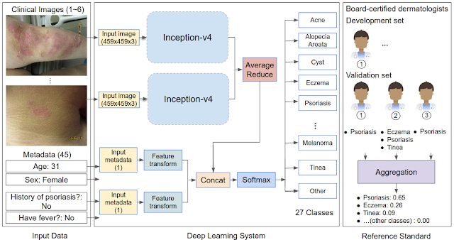
To render this prediction, the DLS processes inputs, including one or more clinical images of the skin abnormality and up to 45 types of metadata (self-reported components of the medical history such as age, sex, symptoms, etc.). For each case, multiple images were processed using the Inception-v4 neural network architecture and combined with feature-transformed metadata, for use in the classification layer. In our study, we developed and evaluated the DLS with 17,777 de-identified cases that were primarily referred from primary care clinics to a teledermatology service. Data from 2010-2017 were used for training and data from 2017-2018 for evaluation. During model training, the DLS leveraged over 50,000 differential diagnoses provided by over 40 dermatologists.

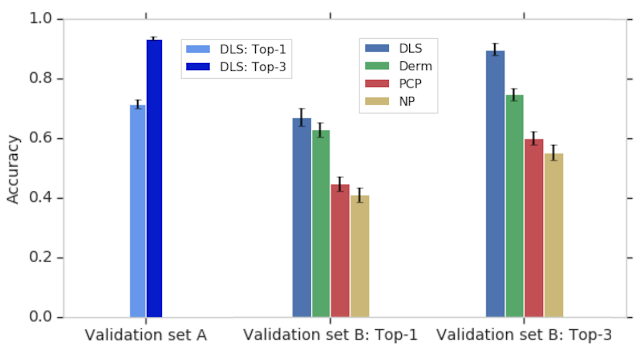
To evaluate the DLS’s accuracy, we compared it to a rigorous reference standard based on the diagnoses from three U.S. board-certified dermatologists. In total, dermatologists provided differential diagnoses for 3,756 cases (“Validation set A”), and these diagnoses were aggregated via a voting process to derive the ground truth labels. The DLS’s ranked list of skin conditions was compared with this dermatologist-derived differential diagnosis, achieving 71% and 93% top-1 and top-3 accuracies, respectively.

Schematic of the DLS and how the reference standard (ground truth) was derived via the voting of three board-certified dermatologists for each case in the validation set.

Comparison to Professional Evaluations
In this study, we also compared the accuracy of the DLS to that of three categories of clinicians on a subset of the validation A dataset (“Validation set B”): dermatologists, primary care physicians (PCPs), and nurse practitioners (NPs) — all chosen randomly and representing a range of experience, training, and diagnostic accuracy. Because typical differential diagnoses provided by clinicians only contain up to three diagnoses, we compared only the top three predictions by the DLS with the clinicians. The DLS achieved a top-3 diagnostic accuracy of 90% on the validation B dataset, which was comparable to dermatologists and substantially higher than primary care physicians (PCPs) and nurse practitioners (NPs)—75%, 60%, and 55%, respectively, for the 6 clinicians in each group. This high top-3 accuracy suggests that the DLS may help prompt clinicians (including dermatologists) to consider possibilities that were not originally in their differential diagnoses, thus improving diagnostic accuracy and condition management.

The DLS’s leading (top-1) differential diagnosis is substantially higher than PCPs and NPs, and on par with dermatologists. This accuracy increases substantially when we look at the DLS’s top-3 accuracy, suggesting that in the majority of cases the DLS’s ranked list of diagnoses contains the correct ground truth answer for the case.

Assessing Demographic Performance
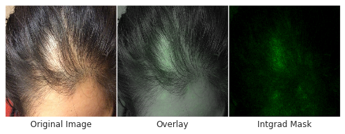
Skin type, in particular, is highly relevant to dermatology, where visual assessment of the skin itself is crucial to diagnosis. To evaluate potential bias towards skin type, we examined DLS performance based on the Fitzpatrick skin type, which is a scale that ranges from Type I (“pale white, always burns, never tans”) to Type VI (“darkest brown, never burns”). To ensure sufficient numbers of cases on which to draw convincing conclusions, we focused on skin types that represented at least 5% of the data — Fitzpatrick skin types II through IV. On these categories, the DLS’s accuracy was similar, with a top-1 accuracy ranging from 69-72%, and the top-3 accuracy from 91-94%. Encouragingly, the DLS also remained accurate in patient subgroups for which significant numbers (at least 5%) were present in the dataset based on other self-reported demographic information: age, sex, and race/ethnicities. As further qualitative analysis, we assessed via saliency (explanation) techniques that the DLS was reassuringly “focusing” on the abnormalities instead of on skin tone.

Left: An example of a case with hair loss that was challenging for non-specialists to arrive at the specific diagnosis, which is necessary for determining appropriate treatment. Right: An image with regions highlighted in green showing the areas that the DLS identified as important and used to make its prediction. Center: The combined image, which indicates that the DLS mostly focused on the area with hair loss to make this prediction, instead of on forehead skin color, for example, which may indicate potential bias.

Incorporating Multiple Data Types
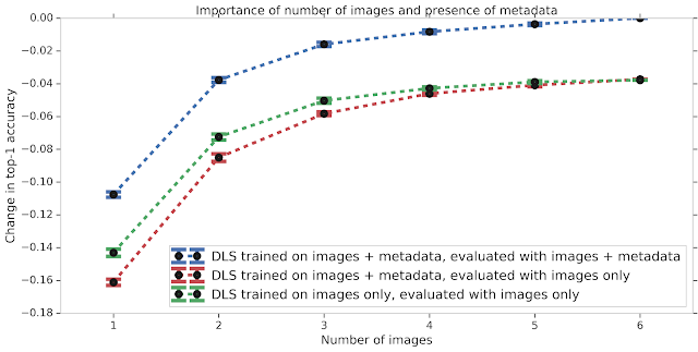
We also studied the effect of different types of input data on the DLS performance. Much like how having images from several angles can help a teledermatologist more accurately diagnose a skin condition, the accuracy of the DLS improves with increasing number of images. If metadata (e.g., the medical history) is missing, the model does not perform as well. This accuracy gap, which may occur in scenarios where no medical history is available, can be partially mitigated by training the DLS with only images. Nevertheless, this data suggests that providing the answers to a few questions about the skin condition can substantially improve the DLS accuracy.

The DLS performance improves when more images (blue line) or metadata (blue compared with red line) are present. In the absence of metadata as input, training a separate DLS using images alone leads to a marginal improvement compared to the current DLS (green line).

Future Work and Applications
Though these results are very promising, much work remains ahead. First, as reflective of real-world practice, the relative rarity of skin cancer such as melanoma in our dataset hindered our ability to train an accurate system to detect cancer. Related to this, the skin cancer labels in our dataset were not biopsy-proven, limiting the quality of the ground truth in this regard. Second, while our dataset did contain a variety of Fitzpatrick skin types, some skin types were too rare in this dataset to allow meaningful training or analysis. Finally, the validation dataset was from one teledermatology service. Though 17 primary care locations across two states were included, additional validation on cases from a wider geographical region will be critical. We believe these limitations can be addressed by including more cases of biopsy-proven skin cancers in the training and validation sets, and including cases representative of additional Fitzpatrick skin types and from other clinical centers.

The success of deep learning to inform the differential diagnosis of skin disease is highly encouraging of such a tool’s potential to assist clinicians. For example, such a DLS could help triage cases to guide prioritization for clinical care or could help non-dermatologists initiate dermatologic care more accurately and potentially improve access. Though significant work remains, we are excited for future efforts in examining the usefulness of such a system for clinicians. For research collaboration inquiries, please contact dermatology-research@google.com.

Acknowledgements
This work involved the efforts of a multidisciplinary team of software engineers, researchers, clinicians and cross functional contributors. Key contributors to this project include Yuan Liu, Ayush Jain, Clara Eng, David H. Way, Kang Lee, Peggy Bui, Kimberly Kanada, Guilherme de Oliveira Marinho, Jessica Gallegos, Sara Gabriele, Vishakha Gupta, Nalini Singh, Vivek Natarajan, Rainer Hofmann-Wellenhof, Greg S. Corrado, Lily H. Peng, Dale R. Webster, Dennis Ai, Susan Huang, Yun Liu, R. Carter Dunn and David Coz. The authors would like to acknowledge William Chen, Jessica Yoshimi, Xiang Ji and Quang Duong for software infrastructure support for data collection. Thanks also go to Genevieve Foti, Ken Su, T Saensuksopa, Devon Wang, Yi Gao and Linh Tran. Last but not least, this work would not have been possible without the participation of the dermatologists, primary care physicians, nurse practitioners who reviewed cases for this study, Sabina Bis who helped to establish the skin condition mapping and Amy Paller who provided feedback on the manuscript.

While people can easily recognize what activities are taking place in videos and anticipate what events may happen next, it is much more difficult for machines. Yet, increasingly, it is important for machines to understand the contents and dynamics of videos for applications, such as temporal localization, action detection and navigation for self-driving cars. In order to train neural networks to perform such tasks, it is common to use supervised training, in which the training data consists of videos that have been meticulously labeled by people on a frame-by-frame basis. Such annotations are hard to acquire at scale. Consequently, there is much interest in self-supervised learning, in which models are trained on various proxy tasks, and the supervision of those tasks naturally resides in the data itself.

In “VideoBERT: A Joint Model for Video and Language Representation Learning” (VideoBERT) and “Contrastive Bidirectional Transformer for Temporal Representation Learning” (CBT), we propose to learn temporal representations from unlabeled videos. The goal is to discover high-level semantic features that correspond to actions and events that unfold over longer time scales. To accomplish this, we exploit the key insight that human language has evolved words to describe high-level objects and events. In videos, speech tends to be temporally aligned with the visual signals, and can be extracted by using off-the-shelf automatic speech recognition (ASR) systems, and thus provides a natural source of self-supervision. Our model is an example of cross-modal learning, as it jointly utilizes the signals from visual and audio (speech) modalities during training.

Image frames and human speech from the same video locations are often semantically aligned. The alignment is non-exhaustive and sometimes noisy, which we hope to mitigate by pretraining on larger datasets. For the left example, the ASR output is, “Keep rolling tight and squeeze the air out to its side and you can kind of pull a little bit.”, where the actions are captured by speech but the objects are not. For the right example, the ASR output is, “This is where you need to be patient patient patient,” which is not related to the visual content at all.

A BERT Model for Videos
The first step of representation learning is to define a proxy task that leads the model to learn temporal dynamics and cross-modal semantic correspondence from long, unlabeled videos. To this end, we generalize the Bidirectional Encoder Representations from Transformers (BERT) model. The BERT model has shown state-of-the-art performance on various natural language processing tasks, by applying the Transformer architecture to encode long sequences, and pretraining on a corpus containing a large amount of text. BERT uses the cloze test as its proxy task, in which the BERT model is forced to predict missing words from context bidirectionally, instead of just predicting the next word in a sequence.

To do this, we generalize the BERT training objective, using image frames combined with the ASR sentence output at the same locations to compose cross-modal “sentences”. The image frames are converted into visual tokens with durations of 1.5 seconds, based on visual feature similarities. They are then concatenated with the ASR word tokens. We train the VideoBERT model to fill out the missing tokens from the visual-text sentences. Our hypothesis, which our experiments support, is that by pretraining on this proxy task, the model learns to reason about longer-range temporal dynamics (visual cloze) and high-level semantics (visual-text cloze).

Illustration of VideoBERT in the context of a video and text masked token prediction, or cloze, task. Bottom: visual and text (ASR) tokens from the same locations of videos are concatenated to form the inputs to VideoBERT. Some visual and text tokens are masked out. Middle: VideoBERT applies the Transformer architecture to jointly encode bidirectional visual-text context. Yellow and pink boxes correspond to the input and output embeddings, respectively. Top: the training objective is to recover the correct tokens for the masked locations.

Inspecting the VideoBERT Model
We trained VideoBERT on over one million instructional videos, such as cooking, gardening and vehicle repair. Once trained, one can inspect what the VideoBERT model learns on a number of tasks to verify that the output accurately reflects the video content. For example, text-to-video prediction can be used to automatically generate a set of instructions (such as a recipe) from video, yielding video segments (tokens) that reflect what is described at each step. In addition, video-to-video prediction can be used to visualize possible future content based on an initial video token.

Qualitative results from VideoBERT, pretrained on cooking videos. Top: Given some recipe text, we generate a sequence of visual tokens. Bottom: Given a visual token, we show the top three future tokens forecast by VideoBERT at different time scales. In this case, the model predicts that a bowl of flour and cocoa powder may be baked in an oven, and may become a brownie or cupcake. We visualize the visual tokens using the images from the training set closest to the tokens in feature space.

To verify if VideoBERT learns semantic correspondences between videos and text, we tested its “zero-shot” classification accuracy on a cooking video dataset in which neither the videos nor annotations were used during pre-training. To perform classification, the video tokens were concatenated with a template sentence “now let me show you how to [MASK] the [MASK]” and the predicted verb and noun tokens were extracted. The VideoBERT model matched the top-5 accuracy of a fully-supervised baseline, indicating that the model is able to perform competitively in this “zero-shot” setting.

Transfer Learning with Contrastive Bidirectional Transformers
While VideoBERT showed impressive results in learning how to automatically label and predict video content, we noticed that the visual tokens used by VideoBERT can lose fine-grained visual information, such as smaller objects and subtle motions. To explore this, we propose the Contrastive Bidirectional Transformers (CBT) model which removes this tokenization step, and further evaluated the quality of learned representations by transfer learning on downstream tasks. CBT applies a different loss function, the contrastive loss, in order to maximize the mutual information between the masked positions and the rest of cross-modal sentences. We evaluated the learned representations for a diverse set of tasks (e.g., action segmentation, action anticipation and video captioning) and on various video datasets. The CBT approach outperforms previous state-of-the-art by significant margins on most benchmarks. We observe that: (1) the cross-modal objective is important for transfer learning performance; (2) a bigger and more diverse pre-training set leads to better representations; (3) compared with baseline methods such as average pooling or LSTMs, the CBT model is much better at utilizing long temporal context.

Action anticipation accuracy with the CBT approach from untrimmed videos with 200 activity classes. We compare with AvgPool and LSTM, and report performance when the observation time is 15, 30, 45 and 72 seconds.

Conclusion & future work
Our results demonstrate the power of the BERT model for learning visual-linguistic and visual representations from unlabeled videos. We find that our models are not only useful for zero-shot action classification and recipe generation, but the learned temporal representations also transfer well to various downstream tasks, such as action anticipation. Future work includes learning low-level visual features jointly with long-term temporal representations, which enables better adaptation to the video context. Furthermore, we plan to expand the number of pre-training videos to be larger and more diverse.

Acknowledgements
The core team includes Chen Sun, Fabien Baradel, Austin Myers, Carl Vondrick, Kevin Murphy and Cordelia Schmid. We would like to thank Jack Hessel, Bo Pang, Radu Soricut, Baris Sumengen, Zhenhai Zhu, and the BERT team for sharing amazing tools that greatly facilitated our experiments. We also thank Justin Gilmer, Abhishek Kumar, Ben Poole, David Ross, and Rahul Sukthankar for helpful discussions.

Much of classical machine learning (ML) focuses on utilizing available data to make more accurate predictions. More recently, researchers have considered other important objectives, such as how to design algorithms to be small, efficient, and robust. With these goals in mind, a natural research objective is the design of a system on top of neural networks that efficiently stores information encoded within—in other words, a mechanism to compute a succinct summary (a “sketch”) of how a complex deep network processes its inputs. Sketching is a rich field of study that dates back to the foundational work of Alon, Matias, and Szegedy, which can enable neural networks to efficiently summarize information about their inputs.

For example: Imagine stepping into a room and briefly viewing the objects within. Modern machine learning is excellent at answering immediate questions, known at training time, about this scene: “Is there a cat? How big is said cat?” Now, suppose we view this room every day over the course of a year. People can reminisce about the times they saw the room: “How often did the room contain a cat? Was it usually morning or night when we saw the room?”. However, can one design systems that are also capable of efficiently answering such memory-based questions even if they are unknown at training time?

In “Recursive Sketches for Modular Deep Learning”, recently presented at ICML 2019, we explore how to succinctly summarize how a machine learning model understands its input. We do this by augmenting an existing (already trained) machine learning model with “sketches” of its computation, using them to efficiently answer memory-based questions—for example, image-to-image-similarity and summary statistics—despite the fact that they take up much less memory than storing the entire original computation.

Basic Sketching Algorithms
In general, sketching algorithms take a vector x and produce an output sketch vector that behaves like x but whose storage cost is much smaller. The fact that the storage cost is much smaller allows one to succinctly store information about the network, which is critical for efficiently answering memory-based questions. In the simplest case, a linear sketch x is given by the matrix-vector product Ax where A is a wide matrix, i.e., the number of columns is equal to the original dimension of x and the number of rows is equal to the new reduced dimension. Such methods have led to a variety of efficient algorithms for basic tasks on massive datasets, such as estimating fundamental statistics (e.g., histogram, quantiles and interquartile range), finding popular items (known as frequent elements), as well as estimating the number of distinct elements (known as support size) and the related tasks of norms and entropy estimation.

A simple method to sketch the vector x is to multiply it by a wide matrix A to produce a lower-dimensional vector y.

This basic approach works well in the relatively simple case of linear regression, where it is possible to identify important data dimensions simply by the magnitude of weights (under the common assumption that they have uniform variance). However, many modern machine learning models are actually deep neural networks and are based on high-dimensional embeddings (such as Word2Vec, Image Embeddings, Glove, DeepWalk and BERT), which makes the task of summarizing the operation of the model on the input much more difficult. However, a large subset of these more complex networks are modular, allowing us to generate accurate sketches of their behavior, in spite of their complexity.

Neural Network Modularity
A modular deep network consists of several independent neural networks (modules) that only communicate via one’s output serving as another’s input. This concept has inspired several practical architectures, including Neural Modular Networks, Capsule Neural Networks and PathNet. It is also possible to split other canonical architectures to view them as modular networks and apply our approach. For example, convolutional neural networks (CNNs) are traditionally understood to behave in a modular fashion; they detect basic concepts and attributes in their lower layers and build up to detecting more complex objects in their higher layers. In this view, the convolution kernels correspond to modules. A cartoon depiction of a modular network is given below.

This is a cartoon depiction of a modular network for image processing. Data flows from the bottom of the figure to the top through the modules represented with blue boxes. Note that modules in the lower layers correspond to basic objects, such as edges in an image, while modules in upper layers correspond to more complex objects, like humans or cats. Also notice that in this imaginary modular network, the output of the face module is generic enough to be used by both the human and cat modules.

Sketch Requirements
To optimize our approach for these modular networks, we identified several desired properties that a network sketch should satisfy:

• Sketch-to-Sketch Similarity: The sketches of two unrelated network operations (either in terms of the present modules or in terms of the attribute vectors) should be very different; on the other hand, the sketches of two similar network operations should be very close.
• Attribute Recovery: The attribute vector, e.g., the activations of any node of the graph can be approximately recovered from the top-level sketch.
• Summary Statistics: If there are multiple similar objects, we can recover summary statistics about them. For example, if an image has multiple cats, we can count how many there are. Note that we want to do this without knowing the questions ahead of time.
• Graceful Erasure: Erasing a suffix of the top-level sketch maintains the above properties (but would smoothly increase the error).
• Network Recovery: Given sufficiently many (input, sketch) pairs, the wiring of the edges of the network as well as the sketch function can be approximately recovered.

This is a 2D cartoon depiction of the sketch-to-sketch similarity property. Each vector represents a sketch and related sketches are more likely to cluster together.

The Sketching Mechanism
The sketching mechanism we propose can be applied to a pre-trained modular network. It produces a single top-level sketch summarizing the operation of this network, simultaneously satisfying all of the desired properties above. To understand how it does this, it helps to first consider a one-layer network. In this case, we ensure that all the information pertaining to a specific node is “packed” into two separate subspaces, one corresponding to the node itself and one corresponding to its associated module. Using suitable projections, the first subspace lets us recover the attributes of the node whereas the second subspace facilitates quick estimates of summary statistics. Both subspaces help enforce the aforementioned sketch-to-sketch similarity property. We demonstrate that these properties hold if all the involved subspaces are chosen independently at random.

Of course, extra care has to be taken when extending this idea to networks with more than one layer—which leads to our recursive sketching mechanism. Due to their recursive nature, these sketches can be “unrolled” to identify sub-components, capturing even complicated network structures. Finally, we utilize a dictionary learning algorithm tailored to our setup to prove that the random subspaces making up the sketching mechanism together with the network architecture can be recovered from a sufficiently large number of (input, sketch) pairs.

Future Directions
The question of succinctly summarizing the operation of a network seems to be closely related to that of model interpretability. It would be interesting to investigate whether ideas from the sketching literature can be applied to this domain. Our sketches could also be organized in a repository to implicitly form a “knowledge graph”, allowing patterns to be identified and quickly retrieved. Moreover, our sketching mechanism allows for seamlessly adding new modules to the sketch repository—it would be interesting to explore whether this feature can have applications to architecture search and evolving network topologies. Finally, our sketches can be viewed as a way of organizing previously encountered information in memory, e.g., images that share the same modules or attributes would share subcomponents of their sketches. This, on a very high level, is similar to the way humans use prior knowledge to recognize objects and generalize to unencountered situations.

Acknowledgements
This work was the joint effort of Badih Ghazi, Rina Panigrahy and Joshua R. Wang.

Automatically generated speech is everywhere, from directions being read out aloud while you are driving, to virtual assistants on your phone or smart speaker devices at home. While much research is being done to try to make synthesized speech sound as natural as possible—such as generating speech for low-resource languages and creating human-like speech with Tacotron 2—how does one evaluate if the generated speech sounds natural or not? The best way to find out is to ask people, who are very good at telling if something sounds natural or not.

In the field of speech synthesis, subjects are routinely asked to listen to samples of synthesized speech and rate their quality. Yet, until now, evaluation of synthesized speech has been done on a sentence by sentence basis. But often one wants to know the quality of a series of sentences that belong together, such as a paragraph in a news article or a turn in a conversation. This is where it gets interesting, as there is more than one way of evaluating sentences that naturally occur in a sequence, and, surprisingly, a rigorous comparison of these different methods has not been carried out. This in turn can hinder research progress in developing products that rely on generated speech.

To address this challenge, we present “Evaluating Long-form Text-to-Speech: Comparing the Ratings of Sentences and Paragraphs”, a publication to appear at SSW10 in which we compare several ways of evaluating synthesized speech for multi-line texts. We find that when a sentence is evaluated as part of a longer text involving several sentences, the outcome is influenced by the way in which the audio sample is presented to the people evaluating it. For example, when the sentence is presented by itself, without any context, the rating people give on average is substantially different from the rating they give when they listen to the same sentence with some context (while the context doesn’t have to be rated).

Evaluating Automatically Generated Speech
To determine the quality of speech signals, it is common practice to ask several human raters to give their opinion for a particular sample, on a 1-to-5 scale. This sample can be automatically generated, but it can also be natural speech (i.e., an actual person saying a sentence out loud), which serves as a control. The scores of all reviewers rating a particular speech sample are averaged to get a Mean Opinion Score (MOS).

Until now, MOS ratings were typically collected per sentence, i.e., raters listened to sentences in isolation to form their opinion. Instead of this typical approach, we consider three different ways of presenting speech samples to raters—both with and without context—and we show that each approach yields different results. The first, presenting the sentence in isolation, is the default method commonly used in the field. An alternative method is to provide the full context for the sentence. In this case, the entire paragraph to which the sentence belongs is included and the ensemble is rated. The final approach is to provide a context-stimulus pair. Here, rather than providing full context, only some context is provided, such as the preceding sentence(s) from the original paragraph.

Interestingly, these three different approaches for presenting speech give different results even when applied to natural speech. This is demonstrated in the figure below, where the MOS scores are presented for natural speech samples rated using the three different methods of presentation. Even though the sentences being rated are identical across the three different settings, the scores are different on average, depending on the context in which they were presented.

MOS results for natural speech from a dataset consisting of news articles. Though the differences appear small, they are significant between all conditions (two-tailed t-test with α=0.05).

Examination of the figure above reveals that raters rarely give top scores (a five) even to recorded human speech, which may be surprising. However, this is a typical result seen in sentence evaluation studies and probably has to do with a more generic pattern of behavior, that people tend to avoid using the extreme ends of a scale, regardless of the task or setting.

When evaluated synthesized speech, the differences are more pronounced.

MOS results for synthesized speech on the same news article dataset used above. All lines are synthesized speech, unless indicated otherwise.

To see if the way context is presented makes a difference, we tried several different ways of providing it: one or two sentences leading up to the sentence to be evaluated, provided as generated speech or real speech. When context is added, the scores get higher (the four blue bars on the left) except when the context presented is real speech, in which case the score drops (the rightmost blue bar). Our hypothesis is that this has to do with an anchoring effect—if the context is very good (real speech) the synthesized speech, in comparison, is perceived as less natural.

Predicting Paragraph Score
When an entire paragraph of synthesized speech is played (the yellow bar), this is perceived as even less natural than in the other settings. Our original hypothesis was a weakest-link argument—the rating is probably as bad as the worst sentence in the paragraph. If that were the case, it should be easy to predict the rating of a paragraph by considering the ratings of the individual sentences in it, perhaps simply taking the minimum value to get the paragraph rating. It turns out, however, that does not work.

The failure of the weakest-link hypothesis may be due to more subtle factors that are difficult to tease out with such a simple approach. To test this, we also trained a machine learning algorithm to predict the paragraph score from the individual sentences. However, this approach, too, was unable to successfully predict paragraph scores reliably.

Conclusion
Evaluating synthesized speech is not straightforward when multiple sentences are involved. The traditional paradigm of rating sentences in isolation does not give the full picture, and one should be aware of anchoring effects when context is provided. Rating full paragraphs might be the most conservative approach. We hope our findings help advance future work in speech synthesis where long-form content is concerned, such as audio book readers and conversational agents.

Acknowledgments
Many thanks to all authors of the paper: Rob Clark, Hanna Silen, Ralph Leith.