Today’s digital assistants are expected to complete tasks and return personalized results across many subjects, such as movie listings, restaurant reservations and travel plans. However, despite tremendous progress in recent years, they have not yet reached human-level understanding. This is due, in part, to the lack of quality training data that accurately reflects the way people express their needs and preferences to a digital assistant. This is because the limitations of such systems bias what we say—we want to be understood, and so tailor our words to what we expect a digital assistant to understand. In other words, the conversations we might observe with today’s digital assistants don’t reach the level of dialog complexity we need to model human-level understanding.

To address this, we’re releasing the Coached Conversational Preference Elicitation (CCPE) and Taskmaster-1 dialog datasets. Both collections make use of a Wizard-of-Oz platform that pairs two people who engage in spoken conversations, just like those one might like to have with a truly effective digital assistant. For both datasets, an in-house Wizard-of-Oz interface was designed to uniquely mimic today’s speech-based digital assistants, preserving the characteristics of spoken dialog in the context of an automated system. Since the human “assistants” understand exactly what the user asks, as any person would, we are able to capture how users would actually express themselves to a “perfect” digital assistant, so that we can continue to improve such systems. Full details of the CCPE dataset are described in our research paper to be published at the 2019 Annual Conference of the Special Interest Group on Discourse and Dialogue, and the Taskmaster-1 dataset is described in detail in a research paper to appear at the 2019 Conference on Empirical Methods in Natural Language Processing.

Preference Elicitation
In the movie-oriented CCPE dataset, individuals posing as a user speak into a microphone and the audio is played directly to the person posing as a digital assistant. The “assistant” types out their response, which is in turn played to the user via text-to-speech. These 2-person dialogs naturally include disfluencies and errors that happen spontaneously between the two parties that are difficult to replicate using synthesized dialog. This creates a collection of natural, yet structured, conversations about people’s movie preferences.

Among the insights into this dataset, we find that the ways in which people describe their preferences are amazingly rich. This dataset is the first to characterize that richness at scale. We also find that preferences do not always match the way digital assistants, or for that matter recommendation sites, characterize options. To put it another way, the filters on your favorite movie website or service probably don’t match the language you would use in describing the sorts of movies that you like when seeking a recommendation from a person.

Task-Oriented Dialog
The Taskmaster-1 dataset makes use of both the methodology described above as well as a one-person, written technique to increase the corpus size and speaker diversity—about 7.7k written “self-dialog” entries and ~5.5k 2-person, spoken dialogs. For written dialogs, we engaged people to create the full conversation themselves based on scenarios outlined for each task, thereby playing roles of both the user and assistant. So, while the spoken dialogs more closely reflect conversational language, written dialogs are both appropriately rich and complex, yet are cheaper and easier to collect. The dataset is based on one of six tasks: ordering pizza, creating auto repair appointments, setting up rides for hire, ordering movie tickets, ordering coffee drinks and making restaurant reservations.

This dataset also uses a simple annotation schema that provides sufficient grounding for the data, while making it easy for workers to apply labels to the dialog consistently. As compared to traditional, detailed strategies that make robust agreement among workers difficult, we focus solely on API arguments for each type of conversation, meaning just the variables required to execute the transaction. For example, in a dialog about scheduling a rideshare, we label the “to” and “from” locations along with the car type (economy, luxury, pool, etc.). For movie tickets, we label the movie name, theater, time, number of tickets, and sometimes the screening type (e.g., 3D or standard). A complete list of labels is included with the corpus release.

It is our hope that these datasets will be useful to the research community for experimentation and analysis in both dialog systems and conversational recommendation.

Acknowledgements
We would like to thank our co-authors and collaborators whose hard work and insights made the release of these datasets possible: Karthik Krishnamoorthi, Krisztian Balog, Chinnadhurai Sankar, Arvind Neelakantan, Amit Dubey, Kyu-Young Kim, Andy Cedilnik, Scott Roy, Muqthar Mohammed, Mohd Majeed, Ashwin Kakarla and Hadar Shemtov.

In 2009, Google created the PhD Fellowship Program to recognize and support outstanding graduate students who are doing exceptional research in Computer Science and related fields who seek to influence the future of technology. Now in its eleventh year, these Fellowships have helped support 450 graduate students globally in North America and Europe, Australia, Asia, Africa and India.

Every year, recipients of the Fellowship are invited to a global summit at our Mountain View campus, where they can learn more about Google’s state-of-the-art research, and network with Google’s research community as well as other PhD Fellows from around the world. Below we share some highlights from our most recent summit, and also announce the latest class of Google PhD Fellows.

Summit Highlights
At this year’s summit event, active Google Fellowship recipients were joined by special guests, FLIP (Diversifying Future Leadership in the Professoriate) Alliance Fellows. Research Director Peter Norvig opened the event with a keynote on the fundamental practice of machine learning, followed by a number of talks by prestigious researchers. Among the list of speakers were Research Scientist Peggy Chi, who spoke about crowdsourcing geographically diverse images for use in training data, Senior Google Fellow and SVP of Google Research and Health Jeff Dean, who discussed using deep learning to solve a variety of challenging research problems at Google, and Research Scientist Vinodkumar Prabhakaran, who presented the ethical implications of machine learning, especially around questions of fairness and accountability. See the complete list of insightful talks delivered by all speakers here.

Google and FLIP Alliance Fellows attending the 2019 PhD Fellowship Summit

Google Fellows had the opportunity to present their work in lightning talks to small groups with common research interests. In addition, Google and FLIP Alliance Fellows came together to share their work with Google researchers and each other during a poster session.

Poster session in full swing

2019 Google PhD Fellows
The Google PhD Fellows represent some of the best and brightest young computer science researchers from around the globe, and it is our ongoing goal to support them as they make their mark on the world. Congratulations to all of this year’s awardees! The complete list of recipients is:

Algorithms, Optimizations and Markets
Aidasadat Mousavifar, EPFL Ecole Polytechnique Fédérale de Lausanne
Peilin Zhong, Columbia University
Siddharth Bhandari, Tata Institute of Fundamental Research
Soheil Behnezhad, University of Maryland at College Park
Zhe Feng, Harvard University

Computational Neuroscience
Caroline Haimerl, New York University
Mai Gamal, Nile University

Human Computer Interaction
Catalin Voss, Stanford University
Hua Hua, Australian National University
Zhanna Sarsenbayeva, University of Melbourne

Machine Learning
Abdulsalam Ometere Latifat, African University of Science and Technology Abuja
Adji Bousso Dieng, Columbia University
Blake Woodworth, Toyota Technological Institute at Chicago
Diana Cai, Princeton University
Francesco Locatello, ETH Zurich
Ihsane Gryech, International University Of Rabat, Morocco
Jaemin Yoo, Seoul National University
Maruan Al-Shedivat, Carnegie Mellon University
Ousseynou Mbaye, Alioune Diop University of Bambey
Redani Mbuvha, University of Johannesburg
Shibani Santurkar, Massachusetts Institute of Technology
Takashi Ishida, University of Tokyo

Machine Perception, Speech Technology and Computer Vision
Anshul Mittal, IIT Delhi
Chenxi Liu, Johns Hopkins University
Kayode Kolawole Olaleye, Stellenbosch University
Ruohan Gao, The University of Texas at Austin
Tiancheng Sun, University of California San Diego
Xuanyi Dong, University of Technology Sydney
Yu Liu, Chinese University of Hong Kong
Zhi Tian, University of Adelaide

Mobile Computing
Naoki Kimura, University of Tokyo

Natural Language Processing
Abigail See, Stanford University
Ananya Sai B, IIT Madras
Byeongchang Kim, Seoul National University
Daniel Patrick Fried, UC Berkeley
Hao Peng, University of Washington
Reinald Kim Amplayo, University of Edinburgh
Sungjoon Park, Korea Advanced Institute of Science and Technology

Privacy and Security
Ajith Suresh, Indian Institute of Science
Itsaka Rakotonirina, Inria Nancy
Milad Nasr, University of Massachusetts Amherst
Sarah Ann Scheffler, Boston University

Programming Technology and Software Engineering
Caroline Lemieux, UC Berkeley
Conrad Watt, University of Cambridge
Umang Mathur, University of Illinois at Urbana-Champaign

Quantum Computing
Amy Greene, Massachusetts Institute of Technology
Leonard Wossnig, University College London
Yuan Su, University of Maryland at College Park

Structured Data and Database Management
Amir Gilad, Tel Aviv University
Nofar Carmeli, Technion
Zhuoyue Zhao, University of Utah

Systems and Networking
Chinmay Kulkarni, University of Utah
Nicolai Oswald, University of Edinburgh
Saksham Agarwal, Cornell University

Around the world, millions of people are coming online for the first time, and many of them are among the 800 million adults worldwide who are unable to read or write, or those who are migrating to towns and cities where they are not able to speak the predominant language. As a smartphone camera-based tool, Google Lens has great potential for helping people who struggle with reading and other language-based challenges. Lens uses computer vision, machine learning and Google’s Knowledge Graph to let people turn the things they see in the real world into a visual search box, enabling them to identify objects like plants and animals, or to copy and paste text from the real world into their phone.

However, in order for Lens to be able to help the greatest number of people, we needed to create a special version that can work on even the most basic smartphones. So at I/O 2019, we announced a new version of Lens designed specifically for use in Google Go—our Search app for entry level devices—and we included a new set of features designed to help people who face reading and other language-based challenges. When users point their camera at text they don’t understand, Lens in Google Go can translate and read it out loud. It even highlights each word as it’s being read so users can follow along. If you want to try out these features for yourself, they are available today via Lens in Google Go. While Google Go was initially available only on Android Go devices and on the Google Play Store in select markets, recently, we made it available globally in the Google Play Store.

To make these reading features work, the Google Go version of Lens needs to be able to capture high quality images on a wide variety of devices, then identify the text, understand its structure, translate and overlay it in context, and finally, read it out loud.

Image Capture
Image capture on entry-level devices, like those that run Android Go, is tricky since it must work on a wide variety of devices, many of which are more resource constrained than flagship phones. To build a universal tool that can reliably capture high-quality images with minimal lag, we made Lens in Google Go an early adopter of a new Android support library called CameraX. Available in Jetpack—a suite of libraries, tools, and guidance for Android developers—CameraX is an abstraction layer over the Android Camera2 API that resolves device compatibility issues so developers don’t have to write their own device-specific code.

Using CameraX, we implemented two capture strategies to balance capture latency against performance impact. On higher-end phones, which are powerful enough to provide a constant stream of high-resolution frames from which to select an image, we’ve made capture instantaneous. On less advanced devices, streaming these frames could cause camera lag since the CPU is less powerful, so we process the frame when the user taps capture to produce a single, on-demand high-resolution image.

Text Recognition
After Lens in Google Go captures an image, it needs to make sense of the shapes and letters that constitute the words, sentences and paragraphs. To do this, the image is scaled down and transferred to the Lens server, where the processing will be performed. Next, optical character recognition (OCR) is applied, which utilizes a region proposal network to detect character level bounding boxes that can be merged into lines for text recognition.

Merging these character boxes into words is a two-step, sequential process. The first step is to apply the Hough Transform, which assumes the text is distributed across parallel lines. The second step uses Text Flow, which instead traces text that may follow a curve by finding the shortest path through a graph of detected text boxes. This ensures that text with a variety of distributions, be they straight, curved or mixed, can be identified and processed.

Because the images captured by Lens in Google Go may include sources such as signage, handwriting or documents, a slew of additional challenges can arise. For example, the text can be obscured, scripts can be uniquely stylized, and images can be blurry. All of these issues can cause the OCR engine to misunderstand various characters within each word. To correct mistakes and improve word accuracy, Lens in Google Go uses the context of surrounding words to make corrections. It also utilizes the Knowledge Graph to provide contextual clues, such as whether a word is likely a proper noun and should not be spell-corrected.

All of these steps, from script detection and direction identification to text recognition, are performed by separable convolutional neural networks (CNNs) with an additional quantized long short-term memory (LSTM) network. And the models are trained on data from a variety of sources, ranging from ReCaptcha to scanned images from Google Books.

Left: Image with bounding box around recognized text. The raw OCR output from this image reads, “Cise is beauti640”. Right: By applying Knowledge Graph in addition to context from nearby words, Lens in Google Go recognizes the words, “life is beautiful”.

Understanding Structure
Once the individual words have been recognized, Lens must determine how to fit them together. The text that people come across in the real world is laid out in many different ways. A newspaper, for example, is laid out into columns, with headlines, article text, and advertisements. Meanwhile, a bus schedule, has one column for destinations and another with times. While understanding text structure comes very naturally to people, computers need to be taught how to comprehend it. Lens uses CNNs to detect coherent text blocks like columns, or text in a consistent style or color. And then, within each block, it uses signals like text-alignment, language, and the geometric relationship of the paragraphs to determine their final reading order.

One of the other challenges in detecting document structure is that people take pictures of text from different angles, often with a warped perspective. This means we cannot revert to off-the-shelf detectors that rely on axis aligned boxes, but must generalize our systems to be able to deal with homographic distortions.

Paragraph segmentation on the front page of a newspaper. Notice how “News Analysis”, which is embedded in the middle of a column, has been identified separately due to its distinct style features.

Translations in Context
To provide users with the most helpful information, translations must be both accurate and contextual. Lens uses Google Translate’s neural machine translation (NMT) algorithms, to translate entire sentences at a time, rather than going word-by-word, in order to preserve proper grammar and diction.

For the translation to be most useful, it needs to be placed in the context of the original text. For example, when translating instructions on an ATM, it is important to know which buttons correspond to which instructions. Part of the challenge is accounting for the fact that the translated text can be much shorter or longer than the original. For example, German sentences tend to be longer than English ones. To accomplish this seamless overlay, Lens redistributes the translation into lines of similar length, and chooses an appropriate font size to match. It also matches the color of the translation and its background with the original text through the use of a heuristic that assumes the background and the text differ in luminosity, and that the background takes up the majority of the space. This allows Lens to classify whether a pixel represents background or text, and then sample the average color from these two regions to ensure the translated text matches the original text.

Reading the Text Out Loud
The final challenge in delivering information in the most helpful way with Lens in Google Go is reading the text aloud. High-fidelity audio is generated using Google Text-to-Speech (TTS), a service that applies machine learning to disambiguate and detected entities such as dates, phone numbers and addresses, and uses that to generate realistic speech based on DeepMind’s WaveNet.

These reading features become more contextual and useful when they are paired with display. Lens utilizes timing annotations from the TTS service that mark the beginning of each word in order to highlight each word on screen as it’s being read, similar to a karaoke machine. Say for example, a user takes a picture of an ATM screen with different labels next to different buttons. This karaoke effect allows users to know which label applies to which button. It may also help users learn how to pronounce the words being translated.

Looking Ahead
Taken together, it is our hope that these features will have a positive impact on the day-to-day lives of millions of people. Moving forward, we will continue to work on further updates to these reading features to make the OCR more precise, including improvements to text structure understanding (e.g. multi-column text) and recognition of Indic scripts. As we address these text challenges, we continue to look for new ways that the combination of machine learning and the smartphone camera can help people as they go about their lives.

When training a neural network to accomplish a given task, be it image classification or reinforcement learning, one typically refines a set of weights associated with each connection within the network. Another approach to creating successful neural networks that has shown substantial progress is neural architecture search, which constructs neural network architectures out of hand-engineered components such as convolutional network components or transformer blocks. It has been shown that neural network architectures built with these components, such as deep convolutional networks, have strong inductive biases for image processing tasks, and can even perform them when their weights are randomly initialized. While neural architecture search produces new ways of arranging hand-engineered components with known inductive biases for the task domain at hand, there has been little progress in the automated discovery of new neural network architectures with such inductive biases, for various task domains.

We can look at analogies to these useful components in examples of nature vs. nurture. Just as certain precocial species in biology—who possess anti-predator behaviors from the moment of birth—can perform complex motor and sensory tasks without learning, perhaps we can construct network architectures that can perform well without training. Of course, these natural (and by analogy, artificial) neural networks are further improved through training, but their ability to perform even without learning shows that they contain biases that make them well-suited to their task.

In “Weight Agnostic Neural Networks” (WANN), we present a first step toward searching specifically for networks with these biases: neural net architectures that can already perform various tasks, even when they use a random shared weight. Our motivation in this work is to question to what extent neural network architectures alone, without learning any weight parameters, can encode solutions for a given task. By exploring such neural network architectures, we present agents that can already perform well in their environment without the need to learn weight parameters. Furthermore, in order to spur progress in this field community, we have also open-sourced the code to reproduce our WANN experiments for the broader research community.

Left: A hand-engineered, fully-connected deep neural network with 2760 weight connections. Using a learning algorithm, we can solve for the set of 2760 weight parameters so that this network can perform the BipedalWalker-v2 task. Right: A weight agnostic neural network architecture with 44 connections that can perform the same Bipedal Walker task. Unlike the fully-connected network, this WANN can still perform the task without the need to train the weight parameters of each connection. In fact, to simplify the training, the WANN is designed to perform when the values of each weight connection are identical, or shared, and it will even function if this shared weight parameter is randomly sampled.

Finding WANNs
We start with a population of minimal neural network architecture candidates, each with very few connections only, and use a well-established topology search algorithm (NEAT), to evolve the architectures by adding single connections and single nodes one by one. The key idea behind WANNs is to search for architectures by de-emphasizing weights. Unlike traditional neural architecture search methods, where all of the weight parameters of new architectures need to be trained using a learning algorithm, we take a simpler and more efficient approach. Here, during the search, all candidate architectures are first assigned a single shared weight value at each iteration, and then optimized to perform well over a wide range of shared weight values.

Operators for searching the space of network topologies Left: A minimal network topology, with input and outputs only partially connected. Middle: Networks are altered in one of three ways: (1) Insert Node: a new node is inserted by splitting an existing connection. (2) Add Connection: a new connection is added by connecting two previously unconnected nodes. (3) Change Activation: the activation function of a hidden node is reassigned. Right: Possible activation functions (linear, step, sin, cosine, Gaussian, tanh, sigmoid, inverse, absolute value, ReLU)

In addition to exploring a range of weight agnostic neural networks, it is important to also look for network architectures that are only as complex as they need to be. We accomplish this by optimizing for both the performance of the networks and their complexity simultaneously, using techniques drawn from multi-objective optimization.

Overview of Weight Agnostic Neural Network Search and corresponding operators for searching the space of network topologies.

Training WANN Architectures
Unlike traditional networks, we can easily train the WANN by simply finding the best single shared weight parameter that maximizes its performance. In the example below, we see that our architecture works (to some extent) for a swing-up cartpole task using constant weights:

As we see in the above figure, while WANNs can perform its task using range of shared weight parameters, the performance is still not comparable to a network that learns weights for each individual connection, as normally done in network training. If we want to further improve its performance, we can use the WANN architecture, and the best shared weight as a starting point to fine-tune the weights of each individual connection using a learning algorithm, like how we would normally train any neural network. Using the weight agnostic property of the network architecture as a starting point, and fine-tuning its performance via learning, may help provide insightful analogies to how animals learn.

The ability for a network architecture to function using only random weights offers other advantages too. For instance, by using copies of the same WANN architecture, but where each copy of the WANN is assigned a different distinct weight value, we can create an ensemble of multiple distinct models for the same task. This ensemble generally achieves better performance than a single model. We illustrate this with an example of an MNIST classifier evolved to work with random weights:

An MNIST classifier evolved to work with random weights.

While a conventional network with random initialization will achieve ~10% accuracy on MNIST, this particular network architecture uses random weights and when applied to MNIST achieves an accuracy much better than chance (> 80%). When an ensemble of WANNs is used, each of which assigned with a different shared weight, the accuracy increases to > 90%.

Even without ensemble methods, collapsing the number of weight values in a network to one allows the network to be rapidly tuned. The ability to quickly fine-tune weights might be useful in continual lifelong learning, where agents acquire, adapt, and transfer skills throughout their lifespan. This makes WANNs particularly well positioned to exploit the Baldwin effect, the evolutionary pressure that rewards individuals predisposed to learn useful behaviors, without being trapped in the computationally expensive trap of ‘learning to learn’.

Conclusion
We hope that this work can serve as a stepping stone to help discover novel fundamental neural network components such as the convolutional network, whose discovery and application have been instrumental to the incredible progress made in deep learning. The computational resources available to the research community have grown significantly since the time convolutional neural networks were discovered. If we are devoting such resources to automated discovery and hope to achieve more than incremental improvements in network architectures, we believe it is also worth searching for with new building blocks, not just their arrangements.

If you are interested to learn more about this work, we invite readers to read our interactive article (or pdf version of the paper for offline reading). In addition to open sourcing these experiments to the research community, we have also released a general Python implementation of NEAT called PrettyNEAT to help interested readers to explore the exciting area of neural network evolution from first principles.

The quality of models produced by machine learning (ML) algorithms directly depends on the quality of the training data, but real world datasets typically contain some amount of noise that introduces challenges for ML models. Noise in the dataset can take several forms from corrupted examples (e.g., lens flare in an image of a cat) to mislabelled examples from when the data was collected (e.g., an image of cat mislabelled as a flerken).

The ability of an ML model to deal with noisy training data depends in great part on the loss function used in the training process. For classification tasks, the standard loss function used for training is the logistic loss. However, this particular loss function falls short when handling noisy training examples due to two unfortunate properties:

1. Outliers far away can dominate the overall loss: The logistic loss function is sensitive to outliers. This is because the loss function value grows without bound as the mislabelled examples (outliers) are far away from the decision boundary. Thus, a single bad example that is located far away from the decision boundary can penalize the training process to the extent that the final trained model learns to compensate for it by stretching the decision boundary and potentially sacrificing the remaining good examples. This “large-margin” noise issue is illustrated in the left panel of the figure below.
2. Mislabeled examples nearby can stretch the decision boundary: The output of the neural network is a vector of activation values, which reflects the margin between the example and the decision boundary for each class. The softmax transfer function is used to convert the activation values into probabilities that an example will belong to each class. As the tail of this transfer function for the logistic loss decays exponentially fast, the training process will tend to stretch the boundary closer to a mislabeled example in order to compensate for its small margin. Consequently, the generalization performance of the network will immediately deteriorate, even with a low level of label noise (right panel below).

We tackle these two problems in a recent paper by introducing a “bi-tempered” generalization of the logistic loss endowed with two tunable parameters that handle those situations well, which we call “temperatures”—t₁, which characterizes boundedness, and t₂ for tail-heaviness (i.e. the rate of decline in the tail of the transfer function). These properties are illustrated below. Setting both t₁ and t₂ to 1.0 recovers the logistic loss function. Setting t₁ lower than 1.0 increases the boundedness and setting t₂ greater than 1.0 makes for a heavier-tailed transfer function. We also introduce this interactive visualization which allows you to visualize the neural network training process with the bi-tempered logistic loss.

Left: Boundedness of the loss function. When t1 is between 0 and 1, exclusive, only a finite amount of loss is incurred for each example, even if they are mislabeled. Shown is t1 = 0.8. Right: Tail-heaviness of the transfer function. The heavy-tailed transfer function applies when t2 = > 1.0 and assigns higher probability for the same amount of activation, thus preventing the boundary from drawing closer to the noisy example. Shown is t2 = 2.0.

To demonstrate the effect of each temperature, we train a two-layer feed-forward neural network for a binary classification problem on a synthetic dataset that contains a circle of points from the first class, and a concentric ring of points from the second class. You can try this yourself on your browser with our interactive visualization. We use the standard logistic loss function, which can be recovered by setting both temperatures equal to 1.0, as well as our bi-tempered logistic loss for training the network. We then demonstrate the effects of each loss function for a clean dataset, a dataset with small-margin noise, large-margin noise, and a dataset with random noise.

Logistic vs. bi-tempered logistic loss: (a) noise-free labels, (b) small-margin label noise, (c) large-margin label noise, and (d) random label noise. The temperature values (t1, t2) for the tempered loss are shown above each figure. We find that for each situation, the decision boundary recovered by training with the bi-tempered logistic loss function is better than before.

Noise Free Case:
We show the results of training the model on the noise-free dataset in column (a), using the logistic loss (top) and the bi-tempered logistic loss (bottom). The white line shows the decision boundary for each model. The values of (t₁, t₂), the temperatures in the bi-tempered loss function, are shown below each column of the figure. Notice that for this choice of temperatures, the loss is bounded and the transfer function is tail-heavy. As can be seen, both losses produce good decision boundaries that successfully separates the two classes.

Small-Margin Noise:
To illustrate the effect of tail-heaviness of the probabilities, we artificially corrupt a random subset of the examples that are near the decision boundary, that is, we flip the labels of these points to the opposite class. The results of training the networks on data with small-margin noise using the logistic loss as well as the bi-tempered loss is shown in column (b).

As can be seen, the logistic loss, due to the lightness of the softmax tail, stretches the boundary closer to the noisy points to compensate for their low probabilities. On the other hand, the bi-tempered loss using only the tail-heavy probability transfer function by adjusting t₂ can successfully avoid the noisy examples. This can be explained by the heavier tail of the tempered exponential function, which assigns reasonably high probability values (and thus, keeps the loss value small) while maintaining the decision boundary away from the noisy examples.

Large-Margin Noise:
Next, we evaluate the performance of the two loss functions for handling large-margin noisy examples. In (c), we randomly corrupt a subset of the examples that are located far away from the decision boundary, the outer side of the ring as well as points near the center).

For this case, we only use the boundedness property of the bi-tempered loss, while keeping the softmax probabilities the same as the logistic loss. The unboundedness of the logistic loss causes the decision boundary to expand towards the noisy points to reduce their loss values. On the other hand, the bounded bi-tempered loss, bounded by adjusting t₁, incurs a finite amount of loss for each noisy example. As a result, the bi-tempered loss can avoid these noisy examples and maintain a good decision boundary.

Random Noise:
Finally, we investigate the effect of random noise in the training data on the two loss functions. Note that random noise comprises both small-margin and large-margin noisy examples. Thus, we use both boundedness and tail-heaviness properties of the bi-tempered loss function by setting the temperatures to (t₁, t₂) = (0.2, 4.0).

As can be seen from the results in the last column, (d), the logistic loss is highly affected by the noisy examples and clearly fails to converge to a good decision boundary. On the other hand, the bi-tempered can recover a decision boundary that is almost identical to the noise-free case.

Conclusion
In this work we constructed a bounded, tempered loss function that can handle large-margin outliers and introduced heavy-tailedness in our new tempered softmax function, which can handle small-margin mislabeled examples. Using our bi-tempered logistic loss, we achieve excellent empirical performance on training neural networks on a number of large standard datasets (please see our paper for full details). Note that the state-of-the-art neural networks have been optimized along with a large variety of variables such as: architecture, transfer function, choice of optimizer, and label smoothing to name just a few. Our method introduces two additional tunable variables, namely (t₁, t₂). We believe that with a systematic “joint optimization” of all commonly tried variables, significant further improvements can be achieved in conjunction with our loss function. This is of course a more long-term goal. We also plan to explore the idea of annealing the temperature parameters over the training process.

Acknowledgements:
This blogpost reflects work with our co-authors Manfred Warmuth, Visiting Researcher and Tomer Koren, Senior Research Scientist, Google Research. Preprint of our paper is available here, which contains theoretical analysis of the loss function and empirical results on standard datasets at scale.

False color maps show up in many applications in computer vision and machine learning, from visualizing depth images to more abstract uses, such as image differencing. Colorizing images helps the human visual system pick out detail, estimate quantitative values, and notice patterns in data in a more intuitive fashion. However, the choice of color map can have a significant impact on a given task. For example, interpretation of “rainbow maps” have been linked to lower accuracy in mission critical applications, such as medical imaging. Still, in many applications, “rainbow maps” are preferred since they show more detail (at the expense of accuracy) and allow for quicker visual assessment.

Left: Disparity image displayed as greyscale. Right: The commonly used Jet rainbow map being used to create a false color image.

One of the most commonly used color mapping algorithms in computer vision applications is Jet, which is high contrast, making it useful for accentuating even weakly distinguished image features. However, if you look at the color map gradient, one can see distinct “bands” of color, most notably in the cyan and yellow regions. This causes sharp transitions when the map is applied to images, which are misleading when the underlying data is actually smoothly varying. Because the rate at which the color changes ‘perceptually’ is not constant, Jet is not perceptually uniform. These effects are even more pronounced for users that are color blind, to the point of making the map ambiguous:

The above image with simulated Protanopia

Today there are many modern alternatives that are uniform and color blind accessible, such as Viridis or Inferno from matplotlib. While these linear lightness maps solve many important issues with Jet, their constraints may make them suboptimal for day to day tasks where the requirements are not as stringent.

Viridis	Inferno

Today we are happy to introduce Turbo, a new colormap that has the desirable properties of Jet while also addressing some of its shortcomings, such as false detail, banding and color blindness ambiguity. Turbo was hand-crafted and fine-tuned to be effective for a variety of visualization tasks. You can find the color map data and usage instructions for Python here and C/C++ here, as well as a polynomial approximation here.

Development
To create the Turbo color map, we created a simple interface that allowed us to interactively adjust the sRGB curves using a 7-knot cubic spline, while comparing the result on a selection of sample images as well as other well known color maps.

Screenshot of the interface used to create and tune Turbo.

This approach provides control while keeping the curve C2 continuous. The resulting color map is not “perceptually linear” in the quantitative sense, but it is more smooth than Jet, without introducing false detail.

Turbo

Jet

Comparison with Common Color Maps
Viridis is a linear color map that is generally recommended when false color is needed because it is pleasant to the eye and it fixes most issues with Jet. Inferno has the same linear properties of Viridis, but is higher contrast, making it better for picking out detail. However, some feel that it can be harsh on the eyes. While this isn’t a concern for publishing, it does affect people’s choice when they must spend extended periods examining visualizations.

Turbo	Jet
Viridis	Inferno

Because of rapid color and lightness changes, Jet accentuates detail in the background that is less apparent with Viridis and even Inferno. Depending on the data, some detail may be lost entirely to the naked eye. The background in the following images is barely distinguishable with Inferno (which is already punchier than Viridis), but clear with Turbo.

Inferno	Turbo

Turbo mimics the lightness profile of Jet, going from low to high back down to low, without banding. As such, its lightness slope is generally double that of Viridis, allowing subtle changes to be more easily seen. This is a valuable feature, since it greatly enhances detail when color can be used to disambiguate the low and high ends.

Turbo	Jet
Viridis	Inferno

The Viridis and Inferno plots are linear, with Inferno exhibiting a higher slope and over a broader range. Jet’s plot is erratic and peaky, and banding can be seen clearly even in the grayscale image. Turbo has a similar asymmetric profile to Jet with the lows darker than the highs.This is intentional, to make cases where low values appear next to high values more distinct. The curvature in the lower region is also different from the higher region, due to the way blues are perceived in comparison to reds.

Although this low-high-low curve increases detail, it comes at the cost of lightness ambiguity. When rendered in grayscale, the coloration will be ambiguous, since some of the lower values will look identical to higher values. Consequently, Turbo is inappropriate for grayscale printing and for people with the rare case of achromatopsia.

Semantic Layers
When examining disparity maps, it is often desirable to compare values on different sides of the image at a glance. This task is much easier when values can be mentally mapped to a distinct semantic color, such as red or blue. Thus, having more colors helps the estimation ease and accuracy.

Turbo	Jet
Viridis	Inferno

With Jet and Turbo, it’s easy to see which objects on the left of the frame are at the same depth as objects on the right, even though there is a visual gap in the middle. For example, you can easily spot which sphere on the left is at the same depth as the ring on the right. This is much harder to determine using Viridis or Inferno, which have far fewer distinct colors. Compared to Jet, Turbo is also much more smooth and has no “false layers” due to banding. You can see this improvement more clearly if the incoming values are quantized:

Left: Quantized Turbo colormap. Up to 33 quantized colors remain distinguishable and smooth in both lightness and hue change. Right: Quantized Jet color map. Many neighboring colors appear the same; Yellow and Cyan colors appear brighter than the rest.

Quick Judging
When doing a quick comparison of two images, it’s much easier to judge the differences in color than in lightness (because our attention system prioritizes hue). For example, imagine we have an output image from a depth estimation algorithm beside the ground truth. With Turbo it’s easy to discern whether or not the two are in agreement and which regions may disagree.

“Output” Viridis	“Ground Truth” Viridis
“Output” Turbo	“Ground Truth” Turbo

In addition, it is easy to estimate quantitative values, since they map to distinguishable and memorable colors.

Diverging Map Use Cases
Although the Turbo color map was designed for sequential use (i.e., values [0-1]), it can be used as a diverging colormap as well, as is needed in difference images, for example. When used this way, zero is green, negative values are shades of blue, and positive values are shades of red. Note, however, that the negative minimum is darker than the positive maximum, so it is not truly balanced.

“Ground Truth” disparity image	Estimated disparity image

Difference Image (ground truth – estimated disparity image), visualized with Turbo

Accessibility for Color Blindness
We tested Turbo using a color blindness simulator and found that for all conditions except Achromatopsia (total color blindness), the map remains distinguishable and smooth. In the case of Achromatopsia, the low and high ends are ambiguous. Since the condition affects 1 in 30,000 individuals (or 0.00003%), Turbo should be usable by 99.997% of the population.

Test Image

Protanomaly	Protanopia
Deuteranomaly	Deuteranopia
Tritanomaly	Tritanopia
Blue cone monochromacy	Achromatopsia

Conclusion
Turbo is a slot-in replacement for Jet, and is intended for day-to-day tasks where perceptual uniformity is not critical, but one still wants a high contrast, smooth visualization of the underlying data. It can be used as a sequential as well as a diverging map, making it a good all-around map to have in the toolbox. You can find the color map data and usage instructions for Python here and for C/C++ here. There is also a polynomial approximation here, for cases where a look-up table may not be desirable.Our team uses it for visualizing disparity maps, error maps, and various other scalar quantities, and we hope you’ll find it useful as well.

Acknowledgements
Ambrus Csaszar stared at many color ramps with me in order to pick the right tradeoffs between uniformity and detail accentuation. Christian Haene integrated the map into our team’s tools, which caused wide usage and thus spurred further improvements. Matthias Kramm and Ruofei Du came up with closed form approximations.

The ability to perceive the shape and motion of hands can be a vital component in improving the user experience across a variety of technological domains and platforms. For example, it can form the basis for sign language understanding and hand gesture control, and can also enable the overlay of digital content and information on top of the physical world in augmented reality. While coming naturally to people, robust real-time hand perception is a decidedly challenging computer vision task, as hands often occlude themselves or each other (e.g. finger/palm occlusions and hand shakes) and lack high contrast patterns.

Today we are announcing the release of a new approach to hand perception, which we previewed CVPR 2019 in June, implemented in MediaPipe—an open source cross platform framework for building pipelines to process perceptual data of different modalities, such as video and audio. This approach provides high-fidelity hand and finger tracking by employing machine learning (ML) to infer 21 3D keypoints of a hand from just a single frame. Whereas current state-of-the-art approaches rely primarily on powerful desktop environments for inference, our method achieves real-time performance on a mobile phone, and even scales to multiple hands. We hope that providing this hand perception functionality to the wider research and development community will result in an emergence of creative use cases, stimulating new applications and new research avenues.

3D hand perception in real-time on a mobile phone via MediaPipe. Our solution uses machine learning to compute 21 3D keypoints of a hand from a video frame. Depth is indicated in grayscale.

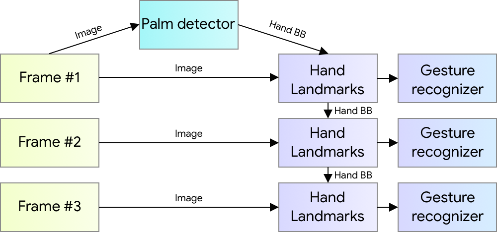
An ML Pipeline for Hand Tracking and Gesture Recognition
Our hand tracking solution utilizes an ML pipeline consisting of several models working together:

• A palm detector model (called BlazePalm) that operates on the full image and returns an oriented hand bounding box.
• A hand landmark model that operates on the cropped image region defined by the palm detector and returns high fidelity 3D hand keypoints.
• A gesture recognizer that classifies the previously computed keypoint configuration into a discrete set of gestures.

This architecture is similar to that employed by our recently published face mesh ML pipeline and that others have used for pose estimation. Providing the accurately cropped palm image to the hand landmark model drastically reduces the need for data augmentation (e.g. rotations, translation and scale) and instead allows the network to dedicate most of its capacity towards coordinate prediction accuracy.

Hand perception pipeline overview.

BlazePalm: Realtime Hand/Palm Detection
To detect initial hand locations, we employ a single-shot detector model called BlazePalm, optimized for mobile real-time uses in a manner similar to BlazeFace, which is also available in MediaPipe. Detecting hands is a decidedly complex task: our model has to work across a variety of hand sizes with a large scale span (~20x) relative to the image frame and be able to detect occluded and self-occluded hands. Whereas faces have high contrast patterns, e.g., in the eye and mouth region, the lack of such features in hands makes it comparatively difficult to detect them reliably from their visual features alone. Instead, providing additional context, like arm, body, or person features, aids accurate hand localization.

Our solution addresses the above challenges using different strategies. First, we train a palm detector instead of a hand detector, since estimating bounding boxes of rigid objects like palms and fists is significantly simpler than detecting hands with articulated fingers. In addition, as palms are smaller objects, the non-maximum suppression algorithm works well even for two-hand self-occlusion cases, like handshakes. Moreover, palms can be modelled using square bounding boxes (anchors in ML terminology) ignoring other aspect ratios, and therefore reducing the number of anchors by a factor of 3-5. Second, an encoder-decoder feature extractor is used for bigger scene context awareness even for small objects (similar to the RetinaNet approach). Lastly, we minimize the focal loss during training to support a large amount of anchors resulting from the high scale variance.

With the above techniques, we achieve an average precision of 95.7% in palm detection. Using a regular cross entropy loss and no decoder gives a baseline of just 86.22%.

Hand Landmark Model
After the palm detection over the whole image our subsequent hand landmark model performs precise keypoint localization of 21 3D hand-knuckle coordinates inside the detected hand regions via regression, that is direct coordinate prediction. The model learns a consistent internal hand pose representation and is robust even to partially visible hands and self-occlusions.

To obtain ground truth data, we have manually annotated ~30K real-world images with 21 3D coordinates, as shown below (we take Z-value from image depth map, if it exists per corresponding coordinate). To better cover the possible hand poses and provide additional supervision on the nature of hand geometry, we also render a high-quality synthetic hand model over various backgrounds and map it to the corresponding 3D coordinates.

Top: Aligned hand crops passed to the tracking network with ground truth annotation. Bottom: Rendered synthetic hand images with ground truth annotation

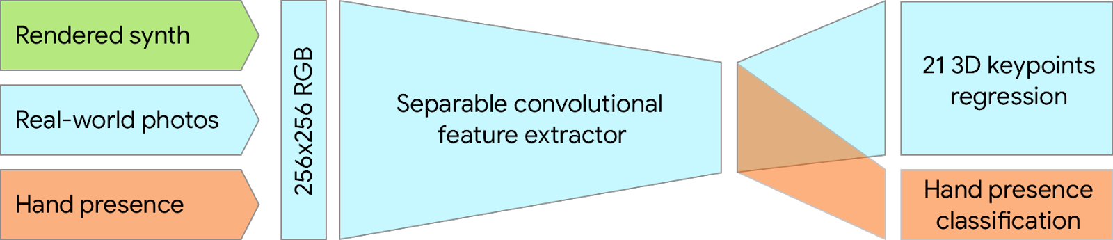
However, purely synthetic data poorly generalizes to the in-the-wild domain. To overcome this problem, we utilize a mixed training schema. A high-level model training diagram is presented in the following figure.

Mixed training schema for hand tracking network. Cropped real-world photos and rendered synthetic images are used as input to predict 21 3D keypoints.

The table below summarizes regression accuracy depending on the nature of the training data. Using both synthetic and real world data results in a significant performance boost.

Gesture Recognition
On top of the predicted hand skeleton, we apply a simple algorithm to derive the gestures. First, the state of each finger, e.g. bent or straight, is determined by the accumulated angles of joints. Then we map the set of finger states to a set of pre-defined gestures. This straightforward yet effective technique allows us to estimate basic static gestures with reasonable quality. The existing pipeline supports counting gestures from multiple cultures, e.g. American, European, and Chinese, and various hand signs including “Thumb up”, closed fist, “OK”, “Rock”, and “Spiderman”.

Implementation via MediaPipe
With MediaPipe, this perception pipeline can be built as a directed graph of modular components, called Calculators. Mediapipe comes with an extendable set of Calculators to solve tasks like model inference, media processing algorithms, and data transformations across a wide variety of devices and platforms. Individual calculators like cropping, rendering and neural network computations can be performed exclusively on the GPU. For example, we employ TFLite GPU inference on most modern phones.

Our MediaPipe graph for hand tracking is shown below. The graph consists of two subgraphs—one for hand detection and one for hand keypoints (i.e., landmark) computation. One key optimization MediaPipe provides is that the palm detector is only run as necessary (fairly infrequently), saving significant computation time. We achieve this by inferring the hand location in the subsequent video frames from the computed hand key points in the current frame, eliminating the need to run the palm detector over each frame. For robustness, the hand tracker model outputs an additional scalar capturing the confidence that a hand is present and reasonably aligned in the input crop. Only when the confidence falls below a certain threshold is the hand detection model reapplied to the whole frame.

The hand landmark model’s output (REJECT_HAND_FLAG) controls when the hand detection model is triggered. This behavior is achieved by MediaPipe’s powerful synchronization building blocks, resulting in high performance and optimal throughput of the ML pipeline.

A highly efficient ML solution that runs in real-time and across a variety of different platforms and form factors involves significantly more complexities than what the above simplified description captures. To this end, we are open sourcing the above hand tracking and gesture recognition pipeline in the MediaPipe framework, accompanied with the relevant end-to-end usage scenario and source code, here. This provides researchers and developers with a complete stack for experimentation and prototyping of novel ideas based on our model.

Future Directions
We plan to extend this technology with more robust and stable tracking, enlarge the amount of gestures we can reliably detect, and support dynamic gestures unfolding in time. We believe that publishing this technology can give an impulse to new creative ideas and applications by the members of the research and developer community at large. We are excited to see what you can build with it!

Acknowledgements
Special thanks to all our team members who worked on the tech with us: Andrey Vakunov, Andrei Tkachenka, Yury Kartynnik, Artsiom Ablavatski, Ivan Grishchenko, Kanstantsin Sokal‎, Mogan Shieh, Ming Guang Yong, Anastasia Tkach, Jonathan Taylor, Sean Fanello, Sofien Bouaziz, Juhyun Lee‎, Chris McClanahan, Jiuqiang Tang‎, Esha Uboweja‎, Hadon Nash‎, Camillo Lugaresi, Michael Hays, Chuo-Ling Chang, Matsvei Zhdanovich and Matthias Grundmann.

Being able to recognize “who said what,” or speaker diarization, is a critical step in understanding audio of human dialog through automated means. For instance, in a medical conversation between doctors and patients, “Yes” uttered by a patient in response to “Have you been taking your heart medications regularly?” has a substantially different implication than a rhetorical “Yes?” from a physician.

Conventional speaker diarization (SD) systems use two stages, the first of which detects changes in the acoustic spectrum to determine when the speakers in a conversation change, and the second of which identifies individual speakers across the conversation. This basic multi-stage approach is almost two decades old, and during that time only the speaker change detection component has improved.

With the recent development of a novel neural network model—the recurrent neural network transducer (RNN-T)—we now have a suitable architecture to improve the performance of speaker diarization addressing some of the limitations of the previous diarization system we presented recently. As reported in our recent paper, “Joint Speech Recognition and Speaker Diarization via Sequence Transduction,” to be presented at Interspeech 2019, we have developed an RNN-T based speaker diarization system and have demonstrated a breakthrough in performance from about 20% to 2% in word diarization error rate—a factor of 10 improvement.

Conventional Speaker Diarization Systems
Conventional speaker diarization systems rely on differences in how people sound acoustically to distinguish the speakers in the conversations. While male and female speakers can be identified relatively easily from their pitch using simple acoustic models (e.g., Gaussian mixture models) in a single stage, speaker diarization systems use a multi-stage approach to distinguish between speakers having potentially similar pitch. First, a change detection algorithm breaks up the conversation into homogeneous segments, hopefully containing only a single speaker, based upon detected vocal characteristics. Then, deep learning models are employed to map segments from each speaker to an embedding vector. Finally, in a clustering stage, these embeddings are grouped together to keep track of the same speaker across the conversation.

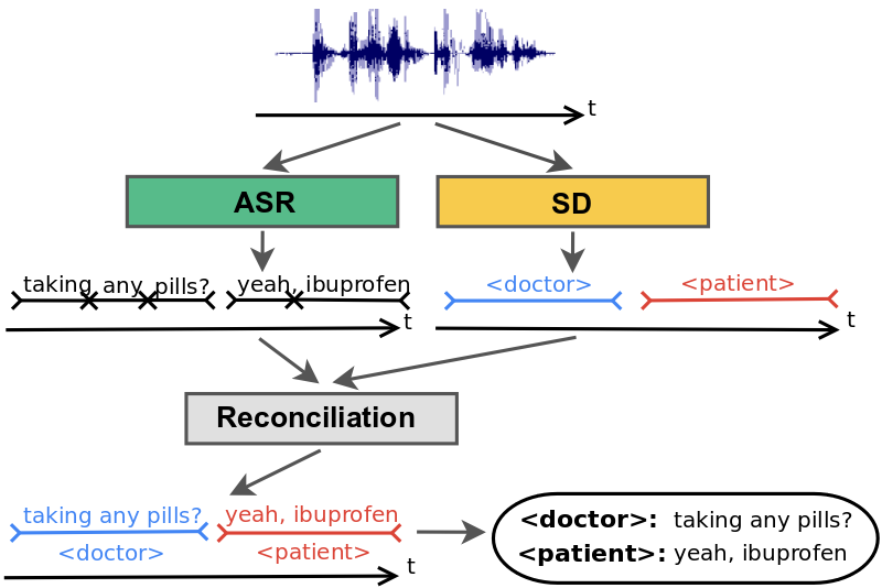
In practice, the speaker diarization system runs in parallel to the automatic speech recognition (ASR) system and the outputs of the two systems are combined to attribute speaker labels to the recognized words.

Conventional speaker diarization system infers speaker labels in the acoustic domain and then overlays the speaker labels on the words generated by a separate ASR system.

There are several limitations with this approach that have hindered progress in this field. First, the conversation needs to be broken up into segments that only contain speech from one speaker. Otherwise, the embedding will not accurately represent the speaker. In practice, however, the change detection algorithm is imperfect, resulting in segments that may contain multiple speakers. Second, the clustering stage requires that the number of speakers be known and is particularly sensitive to the accuracy of this input. Third, the system needs to make a very difficult trade-off between the segment size over which the voice signatures are estimated and the desired model accuracy. The longer the segment, the better the quality of the voice signature, since the model has more information about the speaker. This comes at the risk of attributing short interjections to the wrong speaker, which could have very high consequences, for example, in the context of processing a clinical or financial conversation where affirmation or negation needs to be tracked accurately. Finally, conventional speaker diarization systems do not have an easy mechanism to take advantage of linguistic cues that are particularly prominent in many natural conversations. An utterance, such as “How often have you been taking the medication?” in a clinical conversation is most likely uttered by a medical provider, not a patient. Likewise, the utterance, “When should we turn in the homework?” is most likely uttered by a student, not a teacher. Linguistic cues also signal high probability of changes in speaker turns, for example, after a question.

There are a few exceptions to the conventional speaker diarization system, but one such exception was reported in our recent blog post. In that work, the hidden states of the recurrent neural network (RNN) tracked the speakers, circumventing the weakness of the clustering stage. Our approach takes a different approach and incorporates linguistic cues, as well.

An Integrated Speech Recognition and Speaker Diarization System
We developed a novel and simple model that not only combines acoustic and linguistic cues seamlessly, but also combines speaker diarization and speech recognition into one system. The integrated model does not degrade the speech recognition performance significantly compared to an equivalent recognition only system.

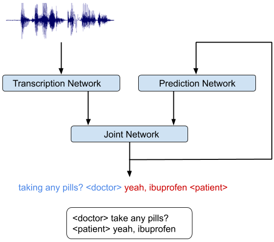
The key insight in our work was to recognize that the RNN-T architecture is well-suited to integrate acoustic and linguistic cues. The RNN-T model consists of three different networks: (1) a transcription network (or encoder) that maps the acoustic frames to a latent representation, (2) a prediction network that predicts the next target label given the previous target labels, and (3) a joint network that combines the output of the previous two networks and generates a probability distribution over the set of output labels at that time step. Note, there is a feedback loop in the architecture (diagram below) where previously recognized words are fed back as input, and this allows the RNN-T model to incorporate linguistic cues, such as the end of a question.

An integrated speech recognition and speaker diarization system where the system jointly infers who spoke when and what.

Training the RNN-T model on accelerators like graphical processing units (GPU) or tensor processing units (TPU) is non-trivial as computation of the loss function requires running the forward-backward algorithm, which includes all possible alignments of the input and the output sequences. This issue was addressed recently in a TPU friendly implementation of the forward-backward algorithm, which recasts the problem as a sequence of matrix multiplications. We also took advantage of an efficient implementation of the RNN-T loss in TensorFlow that allowed quick iterations of model development and trained a very deep network.

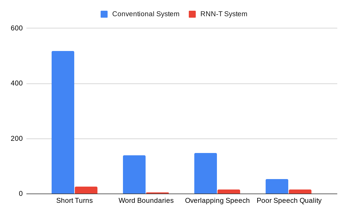
The integrated model can be trained just like a speech recognition system. The reference transcripts for training contain words spoken by a speaker followed by a tag that defines the role of the speaker. For example, “When is the homework due?” ≺student≻, “I expect you to turn them in tomorrow before class,” ≺teacher≻. Once the model is trained with examples of audio and corresponding reference transcripts, a user can feed in the recording of the conversation and expect to see an output in a similar form. Our analyses show that improvements from the RNN-T system impact all categories of errors, including short speaker turns, splitting at the word boundaries, incorrect speaker assignment in the presence of overlapping speech, and poor audio quality. Moreover, the RNN-T system exhibited consistent performance across conversation with substantially lower variance in average error rate per conversation compared to the conventional system.

A comparison of errors committed by the conventional system vs. the RNN-T system, as categorized by human annotators.

Furthermore, this integrated model can predict other labels necessary for generating more reader-friendly ASR transcripts. For example, we have been able to successfully improve our transcripts with punctuation and capitalization symbols using the appropriately matched training data. Our outputs have lower punctuation and capitalization errors than our previous models that were separately trained and added as a post-processing step after ASR.

This model has now become a standard component in our project on understanding medical conversations and is also being adopted more widely in our non-medical speech services.

Acknowledgements
We would like to thank Hagen Soltau without whose contributions this work would not have been possible. This work was performed in collaboration with Google Brain and Speech teams.

The utility of technology is dependent on its accessibility. One key component of accessibility is automatic speech recognition (ASR), which can greatly improve the ability of those with speech impairments to interact with every-day smart devices. However, ASR systems are most often trained from ‘typical’ speech, which means that underrepresented groups, such as those with speech impairments or heavy accents, don’t experience the same degree of utility. For example, amyotrophic lateral sclerosis (ALS) is a disease that can adversely affect a person’s speech—about 25% of people with ALS experiencing slurred speech as their first symptom. In addition, most people with ALS eventually lose the ability to walk, so being able to interact with automated devices from a distance can be very important. Yet current state-of-the-art ASR models can yield high word error rates (WER) for speakers with only a moderate speech impairment from ALS, effectively barring access to ASR reliant technologies.

In “Personalizing ASR for Dysarthric and Accented Speech with Limited Data,” to be presented at Interspeech 2019, we describe some of the research behind Project Euphonia, an ASR platform that performs speech-to-text transcription. This work presents an approach to improve ASR for people with ALS that may also be applicable to many other types of non-standard speech. Using a two-step training approach that starts with a baseline “standard” corpus and then fine-tunes the training with a personalized speech dataset, we have demonstrated significant improvements for speakers with atypical speech over current state-of-the-art models.

A Two-Phased Approach to Training
In order to create ASR models that work on non-standard speech, one needs to overcome two challenges. The first is that within a particular class of atypical speech, be it a regional accent or a speech impairment, for example, individuals can exhibit very different ways of speaking. Our approach deals with this sub-group heterogeneity by training the ASR model in two phases. We start with a high-quality ASR model trained on thousands of hours of standard speech and then we fine-tune parts of the model to an individual with non-standard speech. This approach is similar to that of Parrotron: both systems use end-to-end neural networks to help improve communication and accessibility, but Parrotron focuses exclusively on speech-to-speech, where a person’s speech is converted directly into synthesized speech, rather than text.

The second challenge arises from the difficulty in collecting enough data to train a state-of-the-art recognizer for individuals. Typical speech recognizers are trained on thousands of hours of speech from many different speakers. Acquiring this much data from a single speaker is nearly impossible, especially if the speaker may experience exhaustion from speaking due to a medical condition. Our approach overcomes this issue by first training a base model on a large corpus of typical speech, and then training a personalized model using a much smaller dataset with the targeted non-standard speech characteristics.

The Neural Network Architecture
When developing the models used for training data on atypical speech, we explored two different neural architectures. The first is the RNN-Transducer (RNN-T), a neural network architecture consisting of encoder and decoder networks that has shown good results on numerous ASR tasks. The encoder is bidirectional (i.e., it looks at the entire sentence at once in order to provide context), and thus it requires the entire audio sample to perform speech recognition.

The other architecture we explored was Listen, Attend, and Spell (LAS), which is an attention-based, sequence-to-sequence model that maps sequences of acoustic properties to sequences of languages. This model uses an encoder to convert the sequence of acoustic frames to a sequence of internal representations, and a decoder to convert the sequence of internal representations to linguistic output. The network produces “word pieces”, which are a linguistic representation between graphemes and words.

Comparison of the RNN-Transducer (left) and Listen, Attend, Spell (right) architectures. From Prabhavalkar et al. 2017.

We experimented with fine-tuning the state-of-the-art RNN-T and LAS base models on two types of non-standard speech. In partnership with the ALS Therapy Development Institute, we first collected about 36 hours of audio from 67 speakers who have ALS. The participants recorded themselves on their home computers using custom software while they read sentences from a very restricted language domain. Many phrases were single sentences with simple grammatical structure (e.g., “What time is the basketball game on tonight?”). This is in contrast with unrestricted language domains, which include domain-specific vocabulary (e.g., science talks) and complex language structure (e.g., a debate). The recordings did not include many of the filler words common in normal speech, such as “um” and “uh”.

We also tested accented speech, using the open source L2 Arctic dataset of non-native speech, which consists of 20 speakers with approximately 1 hour of speech per speaker. Each speaker recorded a set of 1150 utterances from the CMU Arctic prompts.

Results
The absolute word error rates on the language-restricted test set is shown below. There is an improvement over the baseline model for very non-standard speech (heavy accents and ALS speech below 3 on the ALS Functional Rating Scale) and moderate improvements in ALS speech that is similar to typical speech. The relative difference between the base model and the fine-tuned model demonstrates that the majority of the improvement comes from the fine-tuning process, except in the case of the RNN-T on the Arctic dataset, where the RNN-T baseline is already strong.

1 Non-native English speech from the L2-Arctic dataset. 2 Low FRS (ALS Functional Rating Scale) speech; intelligible with repeating (FRS 2); Speech combined with non-vocal communication (FRS 1). 3 FRS 3; detectable speech disturbance.

The RNN-T model achieved 91% of the improvement by fine-tuning just two layers, most of which are close to the input. On the accented dataset, fine-tuning the same two layers achieved 86% of the relative improvement compared to fine-tuning the entire network. This is consistent with previous speech work.

Most of the performance gains were achieved early in training. The models we trained were tested on a relatively limited domain of vocabulary and linguistic complexity, so the performance numbers are not necessarily related to how well the models perform on more general tasks. We hope that just fine-tuning part of the network allows it to retain the acoustic and linguistic information from the general speech model, while needing minimal modifications to adapt to a single new speaker. Future work will test this hypothesis.

Low FRS corresponds to the ALS speakers with low intelligibility (FRS 2, 1), while high FRS corresponds to ALS speakers with less severely impacted speech (FRS 3).

Understanding Model Behavior
To better understand how our models improved after fine-tuning, we looked at the pattern of phoneme mistakes. We started by comparing the distribution of phoneme mistakes made by the base ASR model on standard speech to the mistakes made on ALS speech. The SAMPA phonemes with the five largest differences between the ALS data and standard speech are p, U, f, k, and Z, which account for 20% of the deletion mistakes. Similarly, the n and m phonemes together account for 17% of the insertion / substitution mistakes. The same analysis on our fine-tuned models verifies that the unrecognized phoneme distribution is more similar to that of standard speech.

Our analysis shows that there are two aspects to every mistake: which phoneme the system doesn’t understand, and which phoneme the system thinks was said. Imagine having two systems with identical accuracy: one system always thinks that the f phoneme is actually the g phoneme, while another doesn’t know what the f phoneme is and randomly guesses. These two systems will have identical performance and identical distributions of phoneme mistakes, but very different distributions of the predicted phoneme when a mistake is made. Surprisingly, ASR mistakes on ALS speech are far more similar to regular speech mistakes after Euphonia fine-tuning.

Deletion / substitution mistakes per SAMPA phoneme on ALS speech before fine-tuning, ALS speech after fine-tuning, and on typical speech (Librispeech dataset).

Future Work
In the future, we intend to explore additional techniques that can be helpful in the low data regime. We also hope to use phoneme mistakes to weight certain examples during training, or to pick training sentences for people with ALS to record that contain the most common phoneme mistakes. We would like to explore pooling data from multiple speakers with similar conditions.

We hope that continued research in this area will help voice interfaces become accessible to more people, especially those who need it most. One key component to this is collecting data. Anyone 18 or older can help us build better personalized models by donating audio data. If you’re interested, you can fill out this form to allow Google to contact you.

Acknowledgements
This work would not have been possible without the extraordinary effort and support of the ALS Therapy Development Institute and the ALS community, especially Fernando Vieira, Maeve McNally, Taylor Charbonneau, Melissa Nollstadt, and the individuals with ALS who kindly and patiently volunteered their audio. This work builds on the pioneering advances in speech recognition made by Google’s speech team, in particular the recent development and deployment of end-to-end speech recognition models. We are grateful to the Google speech team for advice and collaboration, particularly to Anshuman Tripathi and Hasim Sak who guided us in training the initial models. We’d also like to thank Oran Lang, Omry Tuval, Michael Brenner, Julie Cattiau, Tara Sainath, Ding Zhao, Qiao Liang, Chung-Cheng Chiu, Dan Liebling, Ron Weiss, Anjuli Kannan, Dimitri Kanevsky, Ryan He, Gabor Simko, Benjamin Lee, Françoise Beaufays, Khe Chai Sim, Jimmy Tobin, Chet Gnegy, Jacqueline Huang, Ye Jia, Yu Zhang, Yonghui Wu, Michelle Ramanovich, Rus Heywood, Katrin Tomanek, Bob MacDonald, Pan-Pan Jiang, Ronnie Maor, Rif A. Saurous, Trevor Strohman, Dick Lyon, Avinatan Hassidim, Philip Nelson, and Yossi Matias for their technical contributions and project guidance.

In the last few years there has been great progress in the field of video understanding. For example, supervised learning and powerful deep learning models can be used to classify a number of possible actions in videos, summarizing the entire clip with a single label. However, there exist many scenarios in which we need more than just one label for the entire clip. For example, if a robot is pouring water into a cup, simply recognizing the action of “pouring a liquid” is insufficient to predict when the water will overflow. For that, it is necessary to track frame-by-frame the amount of water in the cup as it is being filled. Similarly, a baseball coach who is comparing stances of pitchers may want to retrieve video frames from the precise moment that the ball leaves the pitchers’ hands. Such applications require models to understand each frame of a video.

However, applying supervised learning to understand each individual frame in a video is expensive, since per-frame labels in videos of the action of interest are needed. This requires that annotators apply fine-grained labels to videos by manually adding unambiguous labels to every frame in each video. Only then can the model be trained, and only on a single action. Training on new actions requires the process to be repeated. With the increasing demand for fine-grained labeling, necessary for applications ranging from robotics to sports analytics, this makes the need for scalable learning algorithms that can understand videos without the tedious labeling process increasingly pertinent.

We propose a potential solution using a self-supervised learning method called Temporal Cycle-Consistency Learning (TCC). This novel approach uses correspondences between examples of similar sequential processes to learn representations particularly well-suited for fine-grained temporal understanding of videos. We are also releasing our TCC codebase to enable end-users to apply our self-supervised learning algorithm to new and novel applications.

Representation Learning Using TCC
A plant growing from a seedling to a tree; the daily routine of getting up, going to work and coming back home; or a person pouring themselves a glass of water are all examples of events that happen in a particular order. Videos capturing such processes provide temporal correspondences across multiple instances of the same process. For example, when pouring a drink one could be reaching for a teapot, a bottle of wine, or a glass of water to pour from. Key moments are common to all pouring videos (e.g., the first touch to the container or the container being lifted from the ground) and exist independent of many varying factors, such as visual changes in viewpoint, scale, container style, or the speed of the event. TCC attempts to find such correspondences across videos of the same action by leveraging the principle of cycle-consistency, which has been applied successfully in many problems in computer vision, to learn useful visual representations by aligning videos.

The objective of this training algorithm is to learn a frame encoder, using any network architecture that processes images, such as ResNet. To do so, we pass all frames of the videos to be aligned through the encoder to produce their corresponding embeddings. We then select two videos for TCC learning, say video 1 (the reference video) and video 2. A reference frame is chosen from video 1 and its nearest neighbor frame (NN₂) from video 2 is found in the embedding space (not pixel space). We then cycle back by finding the nearest neighbor of NN₂ in video 1, which we call NN₁. If the representations are cycle-consistent, then the nearest neighbor frame in video 1 (NN₁) should refer back to the starting reference frame.

We train the embedder using the distance between the starting reference frame and NN₁ as the training signal. As training proceeds, the embeddings improve and reduce the cycle-consistency loss by developing a semantic understanding of each video frame in the context of the action being performed.

Using TCC, we learn embeddings with temporally fine-grained understanding of an action by aligning related videos.

What Does TCC Learn?
In the following figure, we show a model trained using TCC on videos from the Penn Action Dataset of people performing squat exercises. Each point on the left corresponds to frame embeddings, with the highlighted points tracking the embedding of the current video frame. Notice how the embeddings move collectively in spite of many differences in pose, lighting, body and object type. TCC embeddings encode the different phases of squatting without being provided explicit labels.

Right: Input videos of people performing a squat exercise. The video on the top left is the reference. The other videos show nearest neighbor frames (in the TCC embedding space) from other videos of people doing squats. Left: The corresponding frame embeddings move as the action is performed.

Applications of TCC
The learned per-frame embeddings enable an array of interesting applications:

• Few-shot action phase classification
  When few labeled videos are available for training, the few-shot scenario, TCC performs very well. In fact, TCC can classify the phases of different actions with as few as a single labeled video. In the next figure we compare to other supervised and self-supervised learning approaches in the few-shot setting. We find that supervised learning requires about 50 videos with each frame labeled to achieve the same accuracy that self-supervised methods achieve with just one fully labeled video.
  

  Comparison of self-supervised and supervised learning for few-shot action phase classification.

• Unsupervised video alignment
  Aligning or synchronizing videos manually becomes prohibitively difficult as the number of videos increases. Using TCC, many videos can be aligned by selecting the nearest neighbor to each frame in a reference video, without the need for additional labels, as demonstrated in the figure below.
  

  Results of unsupervised video alignment on videos of people pitching baseball using the distance between frames in the TCC space. The reference video used for alignment is shown in the upper left panel.

• Label/modality transfer between videos
  Just as TCC finds similar frames by using a nearest neighbor search in the embedding space, it can transfer metadata associated with any frame in one video to its matching frame in another video. This metadata can be in the form of temporal semantic labels or other modalities, such as sound or text. In the video below we show two examples where we can transfer the sound of liquid being poured into a cup from one video to another.
• Per-frame Retrieval
  With TCC, each frame in a video can be used as a query for retrieval of similar frames by looking up the nearest neighbors in the learned embedding space. The embeddings are powerful enough to differentiate between frames that look quite similar, such as frames just before or after the release of a bowling ball.
  

  We can perform retrieval from videos on a per-frame basis, i.e., any frame can be used to look up similar frames in a large collection of videos. The retrieved nearest neighbors show that the model captures fine-grained differences in the scene.

Release
We are releasing our codebase, which includes implementations of a number of state-of-the-art self-supervised learning methods, including TCC. This codebase will be useful for researchers working on video understanding, as well as artists looking to use machine learning to align videos to create mosaics of people, animals, and objects moving synchronously.

Acknowledgements
This is joint work with Yusuf Aytar, Jonathan Tompson, Pierre Sermanet, and Andrew Zisserman. The authors would like to thank Alexandre Passos, Allen Lavoie, Anelia Angelova, Bryan Seybold, Priya Gupta, Relja Arandjelović, Sergio Guadarrama, Sourish Chaudhuri, and Vincent Vanhoucke for their help with this project. The videos used in this project come from the PennAction dataset. We thank the creators of PennAction for curating such an interesting dataset.