Blog

Learn About Our Meetup

5000+ Members

MEETUPS

LEARN, CONNECT, SHARE

Join our meetup, learn, connect, share, and get to know your Toronto AI community. 

JOB POSTINGS

INDEED POSTINGS

Browse through the latest deep learning, ai, machine learning postings from Indeed for the GTA.

CONTACT

CONNECT WITH US

Are you looking to sponsor space, be a speaker, or volunteer, feel free to give us a shout.

Category: Global

All the Way to 11: NVIDIA GPUs Accelerate 11.11, World’s Biggest Online Shopping Event

Putting AI to work on a massive scale, Alibaba recently harnessed NVIDIA GPUs to serve its customers on 11/11, the year’s largest shopping event.

During Singles Day, as the Nov. 11 shopping event is also known, it generated $38 billion in sales. That’s up by nearly a quarter from last year’s $31 billion, and more than double online sales on Black Friday and Cyber Monday combined.

Singles Day — which has grown from $7 million a decade ago — illustrates the massive scale AI has reached in global online retail, where no player is bigger than Alibaba.

Each day, over 100 million shoppers comb through billions of available products on its site. Activity skyrockets on peak shopping days, when Alibaba’s systems field hundreds of thousands of queries a second.

And AI keeps things humming along, according to Lingjie Xu, Alibaba’s director of heterogeneous computing.

“To ensure these customers have a great user experience, we deploy state-of-the-art AI technology at massive scale using the NVIDIA accelerated computing platform, including T4 GPUs, cuBLAS, customized mixed precision and inference acceleration software,” he said.

“The platform’s intuitive search capabilities and reliable recommendations allow us to support a model six times more complex than in the past, which has driven a 10 percent improvement in click-through rate. Our largest model shows 100 times higher throughput with T4 compared to CPU,” he said.

One key application for Alibaba and other modern online retailers: recommender systems that display items that match user preferences, improving the click-through rate — which is closely watched in the e-commerce industry as a key sales driver.

Every small improvement in click-through rate directly impacts the user experience and revenues. A 10 percent improvement from advanced recommender models that can run in real time, and at incredible scale, is only possible with GPUs.

Alibaba’s teams employ NVIDIA GPUs to support a trio of optimization strategies around resource allocation, model quantization and graph transformation to increase throughput and responsiveness.

This has enabled NVIDIA T4 GPUs to accelerate Alibaba’s wide and deep recommendation model and deliver 780 queries per second. That’s a huge leap from CPU-based inference, which could only deliver three queries per second.

Alibaba has also deployed NVIDIA GPUs to accelerate its systems for automatic advertisement banner-generating, ad recommendation, imaging processing to help identify fake products, language translation, and speech recognition, among others. As the world’s third-largest cloud service provider, Alibaba Cloud provides a wide range of heterogeneous computing products capable of intelligent scheduling, automatic maintenance and real-time capacity expansion.

Alibaba’s far-sighted deployment of NVIDIA’s AI platform is a straw in the wind, indicating what more is to come in a burgeoning range of industries.

Just as its tools filter billions of products for millions of consumers, AI recommenders running on NVIDIA GPUs will find a place among other countless other digital services — app stores, news feeds, restaurant guides and music services among them — keeping customers happy.

Learn more about NVIDIA’s AI inference platform.

The post All the Way to 11: NVIDIA GPUs Accelerate 11.11, World’s Biggest Online Shopping Event appeared first on The Official NVIDIA Blog.

Improving Out-of-Distribution Detection in Machine Learning Models

Successful deployment of machine learning systems requires that the system be able to distinguish between data that is anomalous or significantly different from that used in training. This is particularly important for deep neural network classifiers, which might classify such out-of-distribution (OOD) inputs into in-distribution classes with high confidence. This is critically important when these predictions inform real-world decisions.

For example, one challenging application of machine learning models to real-world applications is bacteria identification based on genomic sequences. Bacteria detection is crucial for diagnosis and treatment of infectious diseases, such as sepsis, and for identifying foodborne pathogens. New bacterial classes continue to be discovered over the years, and while a neural network classifier trained on the known classes achieves high accuracy as measured through cross-validation, deploying a model is challenging, since real-world data is ever evolving and will inevitably contain genomes from unseen classes (OOD inputs) not present in the training data.

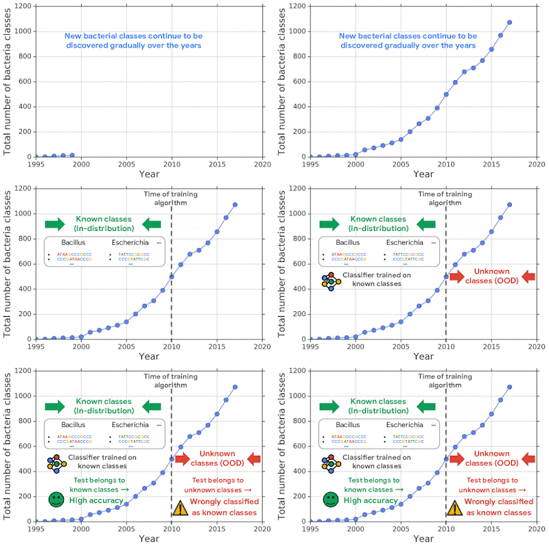
New bacterial classes are gradually discovered over the years. A classifier trained on known classes achieves high accuracy for test inputs belonging to known classes, but can wrongly classify inputs from unknown classes (i.e., out-of-distribution) into known classes with high confidence.

In “Likelihood Ratios for Out-of-Distribution Detection”, presented at NeurIPS 2019, we proposed and released a realistic benchmark dataset of genomic sequences for OOD detection that is inspired by the real-world challenges described above. We tested existing methods for OOD detection using generative models on genomic sequences and found that the likelihood values — i.e., the model’s probability that an input comes from the distribution as estimated using in-distribution data — was often in error. This phenomenon has also been observed in recent work on deep generative models of images. We explain this phenomenon through the effect of background statistics and propose a likelihood-ratio based solution that significantly improves the accuracy of OOD detection.

Why Do Density Models Fail At OOD Detection?
To mimic the real problem and systematically evaluate different methods, we built a new bacterial dataset using data sourced from the publicly available NCBI catalog of prokaryotic genome sequences. To mimic sequencing data, we fragmented genomes into short sequences of 250 base pairs, a length commonly generated by current sequencing technology. We then separated in- and out-of-distribution data by the date of discovery, such that bacterial classes discovered before a cutoff time were defined as in-distribution, and those discovered afterward as OOD.

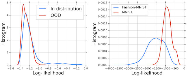
We then trained a deep generative model on in-distribution genomic sequences and examined how well the model discriminated between in- and out-of-distribution inputs by plotting their likelihood values. The histogram of the likelihood for OOD sequences largely overlaps with that of in-distribution sequences, indicating that the generative model was unable to distinguish between the two populations for OOD detection. Similar results were shown in earlier work for deep generative models of images — for instance, a PixelCNN++ model trained on images from Fashion-MNIST dataset (which consists of images of clothing and footwear) assigns higher likelihood to OOD images from the MNIST dataset (which consists of images of digits 0-9).

Left: Histogram of likelihood values for in- and out-of-distribution (OOD) genomic sequences. The likelihood fails to separate in-distribution and OOD genomic sequences. Right: A similar plot for a model trained on Fashion-MNIST and evaluated on MNIST. The model assigns higher likelihood values for OOD (MNIST) than in-distribution images.

When investigating this failure mode, we observed that the likelihood can be confounded by background statistics. To understand the phenomenon more intuitively, assume that an input is composed of two components, (1) a background component characterized by background statistics, and (2) a semantic component characterized by patterns specific to the in-distribution data. For example, an MNIST image can be modeled as background plus semantics. When humans interpret the image, we can easily ignore the background and focus primarily on the semantic information, e.g., the “/” mark in the image below. But the likelihood is calculated for all pixels in an image, including both semantic and background pixels. Though we want to use just the semantic likelihood for decision making, the raw likelihood can be dominated by background.

Left top: Sample images from Fashion-MNIST. Left bottom: Sample images from MNIST. Right: Background and semantic components in an MNIST image.

Likelihood Ratios For OOD Detection
We propose a likelihood ratio method that removes the effect of background and focuses on semantics. First, we train a background model on perturbed inputs. The method for perturbing the input is inspired by genetic mutations, and proceeds by randomly selecting positions in the input and substituting the value with another that has equal probability. For imaging, the values are randomly chosen from the 256 possible pixel values, and for the DNA sequences, the value is selected from the four possible nucleotides (A, T, C, or G). The right amount of perturbation can corrupt the semantic structure in the data, and captures only the background. Then we compute the likelihood ratio between the full model and the background model, and the background component is cancelled out, so that only the likelihood for semantics remains. Likelihood ratio is a background contrastive score, i.e., it captures the significance of the semantics compared to the background.

To qualitatively evaluate the difference between the likelihood and likelihood ratio, we plotted their values for each pixel in the Fashion-MNIST and MNIST datasets, creating heatmaps that have the same size as the images. This allows us to visualize which pixels contribute the most to the two terms, respectively. From the log-likelihood heatmaps, we see that the background pixels contribute much more to the likelihood than the semantic pixels. In hindsight, this is not surprising, since background pixels consist mostly of a string of zeros, a pattern very easily learned by the model. A comparison between the MNIST and Fashion-MNIST heatmaps demonstrates why MNIST returns higher likelihood values — it simply has a lot more background pixels! The likelihood ratio instead focuses more on the semantic pixels.

Left: Log-likelihood heatmaps for Fashion-MNIST and MNIST datasets. Right: The same examples showing heatmaps of the likelihood-ratio. Pixels with higher values are of lighter shades. The likelihood is dominated by the “background” pixels, whereas the likelihood ratio focuses on the “semantic” pixels and is thus better for OOD detection.

Our likelihood ratio method corrects the background effect and significantly improves the OOD detection of MNIST images from an AUROC score of 0.089 to 0.994, based on a PixelCNN++ model trained for Fashion-MNIST. When applied to the genomic benchmark dataset, this method achieves state-of-the-art performance on this challenging problem, when compared to 12 other baseline methods.

For more details, please check out our recent paper at NeurIPS 2019. While our likelihood ratio method reaches state-of-the-art performance on the genomic dataset, it does not yet have high enough accuracy to reach the standards for deployment of the model to real applications. We encourage researchers to contribute their solutions to this important problem and improve the current state-of-the-art. The dataset is available on our GitHub repository.

Acknowledgments
The work described here was authored by Jie Ren, Peter J. Liu, Emily Fertig, Jasper Snoek, Ryan Poplin, Mark A. DePristo, Joshua V. Dillon, Balaji Lakshminarayanan, through a collaboration spanning several teams across Google AI and DeepMind. We are grateful for all the discussions and feedback on this work that we received from the reviewers at NeurIPS 2019, and our colleagues at Google and DeepMind: Alexander A. Alemi, Andreea Gane, Brian Lee, D. Sculley, Eric Jang, Jacob Burnim, Katherine Lee, Matthew D. Hoffman, Noah Fiedel, Rif A. Saurous, Suman Ravuri, Thomas Colthurst, Yaniv Ovadia, along with the Google Brain and TensorFlow teams.

Running distributed TensorFlow training with Amazon SageMaker

TensorFlow is an open-source machine learning (ML) library widely used to develop heavy-weight deep neural networks (DNNs) that require distributed training using multiple GPUs across multiple hosts. Amazon SageMaker is a managed service that simplifies the ML workflow, starting with labeling data using active learning, hyperparameter tuning, distributed training of models, monitoring of training progression, deploying trained models as automatically scalable RESTful services, and centralized management of concurrent ML experiments.

This post focuses on distributed TensorFlow training using Amazon SageMaker.

Overview of concepts

While many of the distributed training concepts in this post are generally applicable across many types of TensorFlow models, this post focuses on distributed TensorFlow training for the Mask R-CNN model on the Common Object in Context (COCO) 2017 dataset.

Model

The Mask R-CNN model is used for object instance segmentation, whereby the model generates pixel-level masks (Sigmoid binary classification) and bounding boxes (Smooth L1 regression) annotated with an object-category (SoftMax classification) to delineate each object instance in an image. Some common use cases for Mask R-CNN include perception in autonomous vehicles, surface defect detection, and analysis of geospatial imagery.

There are three key reasons for selecting the Mask R-CNN model for this post:

  1. Distributed data parallel training of Mask R-CNN on large datasets increases the throughput of images through the training pipeline and reduces training time.
  2. There are many open-source TensorFlow implementations available for the Mask R-CNN model. This post uses Tensorpack Mask/Faster-RCNN implementation as its primary example, but a highly optimized AWS Samples Mask-RCNN is recommended, as well.
  3. The Mask R-CNN model is submitted as part of MLPerf results as a heavy-weight object detection model.

The following graphic is a schematic outline of the Mask R-CNN deep neural network architecture.

Synchronized allreduce of gradients in distributed training

The central challenge in distributed DNN training is that the gradients computed during back propagation across multiple GPUs need to be allreduced (averaged) in a synchronized step before applying the gradients to update the model weights at multiple GPUs across multiple nodes.

The synchronized allreduce algorithm needs to be highly efficient; otherwise, you would lose any training speedup gained from distributed data-parallel training to the inefficiency of a synchronized allreduce step.

There are three key challenges to making a synchronized allreduce algorithm highly efficient:

  • The algorithm needs to scale with the increasing number of nodes and GPUs in the distributed training cluster.
  • The algorithm needs to exploit the topology of high-speed GPU-to-GPU interconnects within a single node.
  • The algorithm needs to efficiently interleave computations on a GPU with communications with other GPUs by efficiently batching the communications with other GPUs.

Uber’s open-source library Horovod addresses these three key challenges as follows:

  • Horovod offers a choice of highly efficient synchronized allreduce algorithms that scale with an increasing number of GPUs and nodes.
  • The Horovod library uses Nvidia Collective Communications Library (NCCL) communication primitives that exploit awareness of Nvidia GPU topology.
  • Horovod includes Tensor Fusion, which efficiently interleaves communication with computation by batching data communication for allreduce.

Horovod is supported with many ML frameworks, including TensorFlow. TensorFlow distribution strategies also use NCCL and provide an alternative to using Horovod to do distributed TensorFlow training. This post uses Horovod.

Training heavy-weight DNNs such as Mask R-CNN require high per GPU memory so you can pump one or more high-resolution images through the training pipeline. They also require high-speed GPU-to-GPU interconnect and high-speed networking interconnecting machines so synchronized allreduce of gradients can be done efficiently. Amazon SageMaker ml.p3.16xlarge and ml.p3dn.24xlarge instance types meet all these requirements. For more information, see Amazon SageMaker ML Instance Types. With eight Nvidia Tesla V100 GPUs, 128–256 GB GPU memory, 25–100 Gbps networking interconnect, and high-speed Nvidia NVLink GPU-to-GPU interconnect, they are ideally suited for distributed TensorFlow training on Amazon SageMaker.

Message Passing Interface

The next challenge in distributed TensorFlow training is the appropriate placement of training algorithm processes across multiple nodes, and associating each algorithm process with a unique global rank. Message Passing Interface (MPI) is a widely used collective communication protocol for parallel computing and is useful in managing a group of training algorithm worker processes across multiple nodes.

MPI is used to distribute training algorithm processes across multiple nodes and associate each algorithm process with a unique global and local rank. Horovod is used to logically pin an algorithm process on a given node to a specific GPU. The logical pinning of each algorithm process to a specific GPU is required for synchronized allreduce of gradients.

The key MPI concept to understand for this post is that MPI uses the mpirun command on a master node to launch concurrent processes across multiple nodes. Using MPI, the master host manages the lifecycle of distributed training processes running across multiple nodes centrally. To use MPI to do distributed training using Amazon SageMaker, you must integrate MPI with the native distributed training capabilities of Amazon SageMaker.

Integrating MPI with Amazon SageMaker distributed training

To understand how to integrate MPI with Amazon SageMaker distributed training, you need an understanding of the following concepts:

  • Amazon SageMaker requires the training algorithm and frameworks packaged in a Docker image.
  • The Docker image must be enabled for Amazon SageMaker training. This enablement is simplified through the use of Amazon SageMaker containers, which is a library that helps create Amazon SageMaker-enabled Docker images.
  • You need to provide an entry point script (typically a Python script) in the Amazon SageMaker training image to act as an intermediary between Amazon SageMaker and your algorithm code.
  • To start training on a given host, Amazon SageMaker runs a Docker container from the training image and invokes the entry point script with entry point environment variables that provide information such as hyperparameters and the location of input data.
  • The entry point script uses the information passed to it in the entry point environment variables to start your algorithm program with the correct args and polls the running algorithm process.
  • When the algorithm process exits, the entry point script exits with the exit code of the algorithm process. Amazon SageMaker uses this exit code to determine the success or failure of the training job.
  • The entry point script redirects the output of the algorithm process’ stdout and stderr to its own stdout. In turn, Amazon SageMaker captures the stdout from the entry point script and sends it to Amazon CloudWatch Logs. Amazon SageMaker parses the stdout output for algorithm metrics defined in the training job and sends the metrics to Amazon CloudWatch metrics.
  • When Amazon SageMaker starts a training job that requests multiple training instances, it creates a set of hosts and logically names each host as algo-k, where k is the global rank of the host. For example, if a training job requests four training instances, Amazon SageMaker names the hosts as algo-1, algo-2, algo-3, and algo-4. The hosts can connect on the network using these hostnames.

In the case of distributed training using MPI, you need a single mpirun command running on the master node (host) that controls the lifecycle of all algorithm processes distributed across multiple nodes, algo-1 through algo-n, where n is the number of training instances requested in your Amazon SageMaker training job. However, Amazon SageMaker is unaware of MPI or any other parallel processing framework you may use to distribute your algorithm processes across multiple nodes. Amazon SageMaker is going to invoke the entry point script on the Docker container running on each node. This means the entry point script needs to be aware of the global rank of its node and execute different logic depending on whether it is invoked on the master node or one of the non-master nodes.

Specifically, for the case of MPI, the entry point script invoked on the master node needs to run the mpirun command to start algorithm processes across all the nodes in the current Amazon SageMaker training job’s host set. The same entry point script when invoked by Amazon SageMaker on any of the non-master nodes periodically checks if the algorithm processes on the non-master node, which the mpirun command manages remotely from the master node, are still running, and exit when they are no longer running.

A master node in MPI is a logical concept, so it is up to the entry point script to designate a host from among all the hosts in the current training job host set as a master node. This designation has to be done in a decentralized manner. A simple approach is to designate algo-1 as the master node and all other hosts as non-master nodes. Because Amazon SageMaker provides each node its logical hostname in the entry point environment variables, it is straightforward for a node to decide if it is the master node or a non-master node.

The train.py included in the accompanying GitHub repo and packaged in the Tensorpack Mask/Faster-RCNN algorithm Docker image follows the logic outlined in this section.

With the background of this conceptual understanding, you’re ready to proceed to the step-by-step tutorial on how to run distributed TensorFlow training for Mask R-CNN using Amazon SageMaker.

Solution overview

This tutorial has the following key steps:

  1. Use an AWS CloudFormation automation script to create a private Amazon VPC and create an Amazon SageMaker notebook instance network attached to this private VPC.
  2. From the Amazon SageMaker notebook instance, launch distributed training jobs in an Amazon SageMaker-managed Amazon VPC network attached to your private VPC. You can use Amazon S3, Amazon EFS, and Amazon FSx as data sources for the training data pipeline.

Prerequisites

The following prerequisites are required:

  1. Create and activate an AWS Account or use an existing AWS account.
  2. Manage your Amazon SageMaker instance limits. You need a minimum of two ml.p3dn.24xlarge or two ml.p3.16xlarge instances; a service limit of four of each is recommended. Keep in mind that the service limit is specific to each AWS Region. This post uses us-west-2.
  3. Clone this post’s GitHub repo and complete the steps in this post. All paths in this post are relative to the GitHub repo root.
  4. Use any AWS Region that supports Amazon SageMaker, EFS, and Amazon FSx. This post uses us-west-2.
  5. Create a new S3 bucket or choose an existing bucket.

Creating an Amazon SageMaker notebook instance attached to a VPC

The first step is to run an AWS CloudFormation automation script to create an Amazon SageMaker notebook instance attached to a private VPC. To run this script, you need IAM user permissions consistent with the Network Administrator function. If you do not have such access, you may need to seek help from your network administrator to run the AWS CloudFormation automation script included in this tutorial. For more information, see AWS Managed Policies for Job Functions.

Use the AWS CloudFormation template cfn-sm.yaml to create an AWS CloudFormation stack that creates a notebook instance attached to a private VPC. You can either create the AWS CloudFormation stack using cfn-sm.yaml in AWS CloudFormation service console, or you can customize variables in stack-sm.sh script and run the script anywhere you have AWS CLI installed.

To use the AWS CLI approach, complete the following steps:

  1. Install AWS CLI and configure it.
  2. In stack-sm.sh, set AWS_REGION to your AWS Region and S3_BUCKET to your S3 bucket. These two variables are required.
  3. Optionally, set the EFS_ID variable if you want to use an existing EFS file system. If you leave EFS_ID blank, a new EFS file system is created. If you chose to use an existing EFS file system, make sure the existing file system does not have any existing mount targets. For more information, see Managing Amazon EFS File Systems.
  4. Optionally, specify GIT_URL to add a GitHub repo to the Amazon SageMaker notebook instance. If the GitHub repo is private, you can specify GIT_USER and GIT_TOKEN variables.
  5. Run the customized stack-sm.sh script to create an AWS CloudFormation stack using AWS CLI.

Save the summary output of the AWS CloudFormation script to use later. You can also view the output under the AWS CloudFormation Stack Outputs tab on the AWS Management Console.

Launching Amazon SageMaker training jobs

In the Amazon SageMaker console, open the notebook instance you created. In this notebook instance, there are three Jupyter notebooks available for training Mask R-CNN:

The training time performance for all three data source options is similar (though not identical) for this post’s choice of Mask R-CNN model and COCO 2017 dataset. The cost profile for each of the data sources is different. The following are differences in terms of the time it takes to set up the training data pipeline:

  • For the S3 data source, each time the training job launches, it takes approximately 20 minutes to replicate the COCO 2017 dataset from your S3 bucket to the storage volumes attached to each training instance.
  • For the EFS data source, it takes approximately 46 minutes to copy the COCO 2017 dataset from your S3 bucket to your EFS file system. You only need to copy this data one time. During training, data is input from the shared EFS file system mounted on all the training instances through a network interface.
  • For Amazon FSx, it takes approximately 10 minutes to create a new Amazon FSx Lustre file system and import the COCO 2017 dataset from your S3 bucket to the new Amazon FSx Lustre file system. You only need to do this one time. During training, data is input from the shared Amazon FSx Lustre file system mounted on all the training instances through a network interface.

If you are not sure which data source option is best for you, start with S3, and explore EFS or Amazon FSx if the training data download time at the start of each training job is not acceptable. Do not assume anything about training time performance for any of the data sources. Training time performance depends on many factors; it is best to experiment and measure it.

In all three cases, the logs and model checkpoints output during training are written to a storage volume attached to each training instance, and upload to your S3 bucket when training is complete. The logs are also fed into Amazon CloudWatch as training progresses that you can review during training. System and algorithm training metrics are fed into Amazon CloudWatch metrics during training, which you can visualize in the Amazon SageMaker service console.

Training results

The following graphs are example results for the two algorithms, after training for 24 epochs on the COCO 2017 dataset.

Below you can see the example results for TensorPack Mask/Faster-RCNN algorithm. The graphs below can be split into three buckets:

  1. Mean average precision (mAP) graphs for bounding box (bbox) prediction for various values of Intersection over Union (IoU), and small, medium, and large object sizes
  2. Mean average precision (mAP) graphs for object instance segmentation (segm) prediction for various values of Intersection over Union (IoU), and  small, medium, and large object sizes
  3. Other metrics related to training loss, or label accuracy

Below you can see the example results for the optimized AWS Samples Mask R-CNN algorithm. The converged mAP metrics shown in the graphs below are almost identical  to the previous algorithm, although the convergence progression is different.

Conclusion

Amazon SageMaker provides a Docker-based, simplified distributed TensorFlow training platform that allows you to focus on your ML algorithm and not be distracted by ancillary concerns such as the mechanics of infrastructure availability and scalability, and concurrent experiment management. When your model is trained, you can use the integrated model deployment capability of Amazon SageMaker to create an automatically scalable RESTful service endpoint for your model and start testing it. For more information, see Deploy a Model on Amazon SageMaker Hosting Services. When your model is ready, you can seamlessly deploy the model RESTful service into production.


About the Author

Ajay Vohra is a Principal Solutions Architect specializing in perception machine learning for autonomous vehicle development. Prior to Amazon, Ajay worked in the area of massively parallel grid-computing for financial risk modeling, and automation of application platform engineering in on-premise data centers.


Improvements to Portrait Mode on the Google Pixel 4 and Pixel 4 XL

Portrait Mode on Pixel phones is a camera feature that allows anyone to take professional-looking shallow depth of field images. Launched on the Pixel 2 and then improved on the Pixel 3 by using machine learning to estimate depth from the camera’s dual-pixel auto-focus system, Portrait Mode draws the viewer’s attention to the subject by blurring out the background. A critical component of this process is knowing how far objects are from the camera, i.e., the depth, so that we know what to keep sharp and what to blur.

With the Pixel 4, we have made two more big improvements to this feature, leveraging both the Pixel 4’s dual cameras and dual-pixel auto-focus system to improve depth estimation, allowing users to take great-looking Portrait Mode shots at near and far distances. We have also improved our bokeh, making it more closely match that of a professional SLR camera.

Pixel 4’s Portrait Mode allows for Portrait Shots at both near and far distances and has SLR-like background blur. (Photos Credit: Alain Saal-Dalma and Mike Milne)

A Short Recap
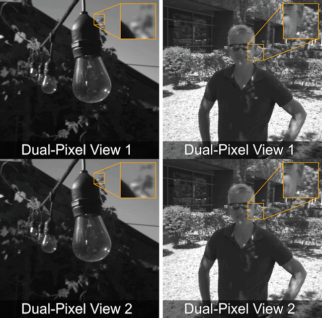
The Pixel 2 and 3 used the camera’s dual-pixel auto-focus system to estimate depth. Dual-pixels work by splitting every pixel in half, such that each half pixel sees a different half of the main lens’ aperture. By reading out each of these half-pixel images separately, you get two slightly different views of the scene. While these views come from a single camera with one lens, it is as if they originate from a virtual pair of cameras placed on either side of the main lens’ aperture. Alternating between these views, the subject stays in the same place while the background appears to move vertically.

The dual-pixel views of the bulb have much more parallax than the views of the man because the bulb is much closer to the camera.

This motion is called parallax and its magnitude depends on depth. One can estimate parallax and thus depth by finding corresponding pixels between the views. Because parallax decreases with object distance, it is easier to estimate depth for near objects like the bulb. Parallax also depends on the length of the stereo baseline, that is the distance between the cameras (or the virtual cameras in the case of dual-pixels). The dual-pixels’ viewpoints have a baseline of less than 1mm, because they are contained inside a single camera’s lens, which is why it’s hard to estimate the depth of far scenes with them and why the two views of the man look almost identical.

Dual Cameras are Complementary to Dual-Pixels
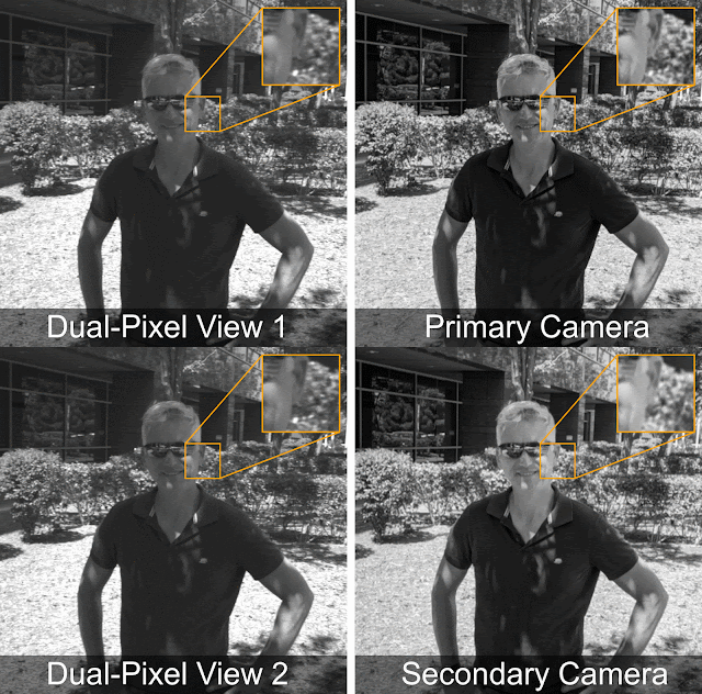
The Pixel 4’s wide and telephoto cameras are 13 mm apart, much greater than the dual-pixel baseline, and so the larger parallax makes it easier to estimate the depth of far objects. In the images below, the parallax between the dual-pixel views is barely visible, while it is obvious between the dual-camera views.

Left: Dual-pixel views. Right: Dual-camera views. The dual-pixel views have only a subtle vertical parallax in the background, while the dual-camera views have much greater horizontal parallax. While this makes it easier to estimate depth in the background, some pixels to the man’s right are visible in only the primary camera’s view making it difficult to estimate depth there.

Even with dual cameras, information gathered by the dual pixels is still useful. The larger the baseline, the more pixels that are visible in one view without a corresponding pixel in the other. For example, the background pixels immediately to the man’s right in the primary camera’s image have no corresponding pixel in the secondary camera’s image. Thus, it is not possible to measure the parallax to estimate the depth for these pixels when using only dual cameras. However, these pixels can still be seen by the dual pixel views, enabling a better estimate of depth in these regions.

Another reason to use both inputs is the aperture problem, described in our previous blog post, which makes it hard to estimate the depth of vertical lines when the stereo baseline is also vertical (or when both are horizontal). On the Pixel 4, the dual-pixel and dual-camera baselines are perpendicular, allowing us to estimate depth for lines of any orientation.

Having this complementary information allows us to estimate the depth of far objects and reduce depth errors for all scenes.

Depth from Dual Cameras and Dual-Pixels
We showed last year how machine learning can be used to estimate depth from dual-pixels. With Portrait Mode on the Pixel 4, we extended this approach to estimate depth from both dual-pixels and dual cameras, using Tensorflow to train a convolutional neural network. The network first separately processes the dual-pixel and dual-camera inputs using two different encoders, a type of neural network that encodes the input into an intermediate representation. Then, a single decoder uses both intermediate representations to compute depth.

Our network to predict depth from dual-pixels and dual-cameras. The network uses two encoders, one for each input and a shared decoder with skip connections and residual blocks.

To force the model to use both inputs, we applied a drop-out technique, where one input is randomly set to zero during training. This teaches the model to work well if one input is unavailable, which could happen if, for example, the subject is too close for the secondary telephoto camera to focus on.

Depth maps from our network where either only one input is provided or both are provided. Top: The two inputs provide depth information for lines in different directions. Bottom: Dual-pixels provide better depth in the regions visible in only one camera, emphasized in the insets. Dual-cameras provide better depth in the background and ground. (Photo Credit: Mike Milne)

The lantern image above shows how having both signals solves the aperture problem. Having one input only allows us to predict depth accurately for lines in one direction (horizontal for dual-pixels and vertical for dual-cameras). With both signals, we can recover the depth on lines in all directions.

With the image of the person, dual-pixels provide better depth information in the occluded regions between the arm and torso, while the large baseline dual cameras provide better depth information in the background and on the ground. This is most noticeable in the upper-left and lower-right corner of depth from dual-pixels. You can find more examples here.

SLR-Like Bokeh
Photographers obsess over the look of the blurred background or bokeh of shallow depth of field images. One of the most noticeable things about high-quality SLR bokeh is that small background highlights turn into bright disks when defocused. Defocusing spreads the light from these highlights into a disk. However, the original highlight is so bright that even when its light is spread into a disk, the disk remains at the bright end of the SLR’s tonal range.

Left: SLRs produce high contrast bokeh disks. Middle: It is hard to make out the disks in our old background blur. Right: Our new bokeh is closer to that of an SLR.

To reproduce this bokeh effect, we replaced each pixel in the original image with a translucent disk whose size is based on depth. In the past, this blurring process was performed after tone mapping, the process by which raw sensor data is converted to an image viewable on a phone screen. Tone mapping compresses the dynamic range of the data, making shadows brighter relative to highlights. Unfortunately, this also results in a loss of information about how bright objects actually were in the scene, making it difficult to produce nice high-contrast bokeh disks. Instead, the bokeh blends in with the background, and does not appear as natural as that from an SLR.

The solution to this problem is to blur the merged raw image produced by HDR+ and then apply tone mapping. In addition to the brighter and more obvious bokeh disks, the background is saturated in the same way as the foreground. Here’s an album showcasing the better blur, which is available on the Pixel 4 and the rear camera of the Pixel 3 and 3a (assuming you have upgraded to version 7.2 of the Google Camera app).

Blurring before tone mapping improves the look of the backgrounds by making it more saturated and by making disks higher contrast.

Try it Yourself
We have made Portrait Mode on the Pixel 4 better by improving depth quality, resulting in fewer errors in the final image and by improving the look of the blurred background. Depth from dual-cameras and dual-pixels only kicks in when the camera is at least 20 cm from the subject, i.e. the minimum focus distance of the secondary telephoto camera. So consider keeping your phone at least that far from the subject to get better quality portrait shots.

Acknowledgments
This work wouldn’t have been possible without Rahul Garg, Sergio Orts Escolano, Sean Fanello, Christian Haene, Shahram Izadi, David Jacobs, Alexander Schiffhauer, Yael Pritch Knaan and Marc Levoy. We would also like to thank the Google Camera team for helping to integrate these algorithms into the Pixel 4. Special thanks to our photographers Mike Milne, Andy Radin, Alain Saal-Dalma, and Alvin Li who took numerous test photographs for us.

Auto-segmenting objects when performing semantic segmentation labeling with Amazon SageMaker Ground Truth

Amazon SageMaker Ground Truth helps you build highly accurate training datasets for machine learning (ML) quickly. Ground Truth offers easy access to third-party and your own human labelers and provides them with built-in workflows and interfaces for common labeling tasks. Additionally, Ground Truth can lower your labeling costs by up to 70% using automatic labeling, which works by training Ground Truth from data humans have labeled so that the service learns to label data independently.

Semantic segmentation is a computer vision ML technique that involves assigning class labels to individual pixels in an image. For example, in video frames captured by a moving vehicle, class labels can include vehicles, pedestrians, roads, traffic signals, buildings, or backgrounds. It provides a high-precision understanding of the locations of different objects in the image and is often used to build perception systems for autonomous vehicles or robotics. To build an ML model for semantic segmentation, it is first necessary to label a large volume of data at the pixel level. This labeling process is complex. It requires skilled labelers and significant time—some images can take up to two hours to label accurately.

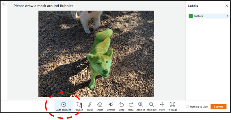
To increase labeling throughput, improve accuracy, and mitigate labeler fatigue, Ground Truth added the auto-segment feature to the semantic segmentation labeling user interface. The auto-segment tool simplifies your task by automatically labeling areas of interest in an image with only minimal input. You can accept, undo, or correct the resulting output from auto-segment. The following screenshot highlights the auto-segmenting feature in your toolbar, and shows that it captured the dog in the image as an object. The label assigned to the dog is Bubbles.

With this new feature, you can work up to ten times faster on semantic segmentation tasks. Instead of drawing a tightly fitting polygon or using the brush tool to capture an object in an image, you draw four points: one at the top-most, bottom-most, left-most, and right-most points of the object. Ground Truth takes these four points as input and uses the Deep Extreme Cut (DEXTR) algorithm to produce a tightly fitting mask around the object. The following demo shows how this tool speeds up the throughput for more complex labeling tasks (video plays at 5x real-time speed).

Conclusion

This post demonstrated the purpose and complexity of the computer vision ML technique called semantic segmentation. The auto-segment feature automates the segmentation of areas of interest in an image with minimal input from the labeler, and speeds up semantic segmentation labeling tasks.

As always, AWS welcomes feedback. Please submit any thoughts or questions in the comments.


About the authors

Krzysztof Chalupka is an applied scientist in the Amazon ML Solutions Lab. He has a PhD in causal inference and computer vision from Caltech. At Amazon, he figures out ways in which computer vision and deep learning can augment human intelligence. His free time is filled with family. He also loves forests, woodworking, and books (trees in all forms).


Vikram Madan is the Product Manager for Amazon SageMaker Ground Truth. He focusing on delivering products that make it easier to build machine learning solutions. In his spare time, he enjoys running long distances and watching documentaries.


AI Calling: How to Kickoff a Career in Data Science

Paul Mahler remembers the day in May 2013 he decided to make the switch.

The former economist was waiting at a bus stop in Washington, D.C., reading the New York Times on his smartphone. He was struck by the story of a statistics professor who wrote an app that let computers review screenplays. It launched the academic into a lucrative new career in Hollywood.

“That seemed like a monumental breakthrough. I decided I wanted to get into data science, too,” said Mahler. Today, he’s a senior data scientist in Silicon Valley, helping NVIDIA’s customers use AI to make their own advances.

Like Mahler, Eyal Toledano made a big left turn a decade into his career. He describes “an existential crisis … I thought if I have any talent, I should try to do something I’m really proud of that’s bigger than myself and even if I fail, I will love every minute,” he said.

Then “an old friend from my undergrad days told me about his diving accident in a remote area and how no one could read his X-rays. He said we should build a database of images [using AI] to facilitate diagnoses in situations where people need this help — it was the first time I devoted myself to a seed of an idea that came from someone else,” Toledano recalled.

The two friends co-founded Zebra Medical Vision in 2014 to apply AI to medical imaging. For Toledano, there was only one way into the emerging field of deep learning.

“Roll up your sleeves, shovel some dirt and join the effort, that’s what helped me — in data science, you really need to get dirty,” he said.

Plenty of Room in the Sandbox

The field is still wide open. Data scientist tops the list of best jobs in America, according to a 2019 ranking from Glassdoor, a service that connects 67 million monthly visitors with 12 million job postings. It pegged median base salary for an entry-level data scientist at $108,000, job satisfaction at 4.3 out of 5 and said there are 6,510 job openings.

The job of data engineer was not far behind at $100,000, 4.2 out of 5 and 4,524 openings.

A 2018 study by recruiters at Burtch Works adds detail to the picture. It estimated starting salaries range from $95,000 to $168,000, depending on skill level. Data scientists come to the job with a wide range of academic backgrounds including math/statistics (25%), computer science and physical science (20% each), engineering (18%) and general business (8%). Nearly half had Ph.D.s and 40 percent held master’s degrees.

“Now that data is the new oil, data science is one of the most important jobs,” said Alen Capalik, co-founder and chief executive of startup FASTDATA.io, a developer of GPU software backed in part by NVIDIA. “Demand is incredible, so the unemployment in data science is zero.”

Like Mahler and Toledano, Capalik jumped in head first. “I just read a lot to understand data, the data pipeline and how customers use their data — different verticals use data differently,” he said.

The Nuts and Bolts

Data scientists are hybrid creatures. Some are statisticians who learned to code. Some are Python wizards learning the nuances of data analytics and machine learning. Others are domain experts who wanted to be part of the next big thing in computing.

All face a common flow of tasks. They must:

  • Identify business problems suited for big data
  • Set up and maintain tool chains
  • Gather large, relevant datasets
  • Structure datasets to address business concerns
  • Select an appropriate AI model family
  • Optimize model hyperparameters
  • Postprocess machine learning models
  • Critically analyze the results

“The unicorn data scientists do it all, from setting up a server to presenting to the board,” said Mahler.

But the reality is the field is quickly segmenting into subtasks. Data engineers work on the frontend of the process, massaging datasets through the so-called extract, transform and load process.

Big operations may employ data librarians, privacy experts and AI pipeline engineers who ensure systems deliver time-sensitive recommendations fast.

“The proliferation of titles is another sign the field is maturing,” said Mahler.

Play a Game, Learn the Job

One of the fastest, most popular ways into the field is to have some fun with AI by entering Kaggle contests, said Mahler. The online matches provide forums with real-world problems and code examples to get started. “People on our NVIDIA RAPIDS product team are continually on Kaggle contests,” he said.

Wins can lead to jobs, too. Owkin, an NVIDIA partner that designs AI software for healthcare, declares on its website, “Our data scientists are among the best in the world, with several Kaggle Masters.”

These days, at least some formal study is recommended. Online courses from fast.ai aim to give experienced programmers a jumpstart into deep learning. Co-founder Rachel Thomas maintains a list of her talks encouraging everyone, especially women, to get into data science.

We compiled our own list of online courses in data science given by the likes of MIT, Google and NVIDIA’s Deep Learning Institute. Here are some other great resources:

“Having a strong grasp of linear algebra, probability and statistical modeling is important for creating and interpreting AI models,” said Mahler. “A lot of employers require a degree in data or computer science and a strong understanding of Python,” he added.

“I was never one to look for degrees,” countered Capalik of FASTDATA.io. “Having real-world experience is better because the first day on a job you will find out things people never showed you in school,” he said.

Both agreed the best data scientists have a strong creative streak. And employers covet data scientists who are imaginative problem solvers.

Getting Picked for a Job

One startup gives job candidates a test of technical skills, but the test is just part of the screening process, said Capalik.

“I like to just look someone in the eye and ask a few questions,” he said. “You want to know if they are a problem solver and can work with a team because data science is a team effort — even Michael Jordan needed a team to win,” he said.

To pass the test and get an interview with Capalik, “you need to know what the data pipeline looks like, how data is collected, where it’s stored and how to work around the nuances and inefficiencies to solve problems with algorithms,” he said.

Toledano of Zebra is suspicious of candidates with pat answers.

“This is an experimental science,” he said. “The results are asymptotic to your ability to run many experiments, so you need to come up with different pieces and ideas quickly and test them in training experiments over and over again,” he said.

“People who want to solve a problem once might be very intelligent, but they will probably miss things. Don’t build a bow and arrow, build a catapult to throw a gazillion arrows — each one a potential solution you can evaluate quickly,” he added

Chris Rowen, a veteran entrepreneur and chief executive of AI startup BabbleLabs, is impressed by candidates who can explain their work. “Understand the theory about why models work on which problems and why,” he advised.

The Developer’s Path

Unlike the pure digital world of IT where answers are right or wrong, data science challenges often have no definitive answer, so they invite the curious who like to explore options and tradeoffs.

Indeed, IT and data science are radically different worlds.

IT departments use carefully structured processes to check code in and out and verify compliance. They write apps once that may be used for years. Data science teams, on the other hand, conduct experiments continuously with models based on probability curves and frequently massage models and datasets.

“Software engineering is more of a straight line while data science is a loop,” said James Kobielus, a veteran market watcher and lead AI analyst at Wikibon.

That said, it’s also true that “data science is the core of the next-generation developer, really,” Kobielus said. Although many subject matter experts jump into data science and learn how to code, “even more people are coming in from general app development,” he said, in part because that’s where the money is these days.

Clouds, Robots and Soft Skills

Whatever path you take, data scientists need to be familiar with the cloud. Many AI projects are born on remote servers using containers and modern orchestration techniques.

And you should understand the latest mobile and edge hardware and its constraints.

“There’s a lot of work going on in robotics using trial-and-error algorithms for reinforcement learning. This is beyond traditional data science, so personnel shortages are more acute there — and computer vision in cameras could not be hotter,” Kobielus said.

A diplomat’s skills for negotiation comes in handy, too. Data scientists are often agents of change, disrupting jobs and processes, so it’s important to make allies.

A Philosophical Shift

It sounds like a lot of work, but don’t be intimidated.

“I don’t know that I’ve made such a huge shift,” said Rowen of BabbleLabs, his first startup to leverage data science.

“The nomenclature has changed. The idea that the problem’s specs are buried in the data is a philosophical shift, but at the root of it, I’m doing something analogous to what I’ve done in much of my career,” he said

In the past Rowen explored the “computational profile of a problem and found the processor to make it work. Now, we turn that upside down. We look at what’s at the heart of a computation and what data we need to do it — that insight carried me into deep learning,” he said.

In a May 2018 talk, fast.ai co-founder Thomas was equally encouraging. Using transfer learning, you can do excellent AI work by training just the last few layers of a neural network, she said. And you don’t always need big data. For example, one system was trained to recognize images of baseball vs. cricket using just 30 pictures.

“The world needs more people in AI, and the barriers are lower than you thought,” she added.

The post AI Calling: How to Kickoff a Career in Data Science appeared first on The Official NVIDIA Blog.
Fairness Indicators: Scalable Infrastructure for Fair ML Systems

While industry and academia continue to explore the benefits of using machine learning (ML) to make better products and tackle important problems, algorithms and the datasets on which they are trained also have the ability to reflect or reinforce unfair biases. For example, consistently flagging non-toxic text comments from certain groups as “spam” or “high toxicity” in a moderation system leads to exclusion of those groups from conversation.

In 2018, we shared how Google uses AI to make products more useful, highlighting AI principles that will guide our work moving forward. The second principle, “Avoid creating or reinforcing unfair bias,” outlines our commitment to reduce unjust biases and minimize their impacts on people.

As part of this commitment, at TensorFlow World, we recently released a beta version of Fairness Indicators, a suite of tools that enable regular computation and visualization of fairness metrics for binary and multi-class classification, helping teams take a first step towards identifying unjust impacts. Fairness Indicators can be used to generate metrics for transparency reporting, such as those used for model cards, to help developers make better decisions about how to deploy models responsibly. Because fairness concerns and evaluations differ case by case, we also include in this release an interactive case study with Jigsaw’s Unintended Bias in Toxicity dataset to illustrate how Fairness Indicators can be used to detect and remediate bias in a production machine learning (ML) model, depending on the context in which it is deployed. Fairness Indicators is now available in beta for you to try for your own use cases.

What is ML Fairness?
Bias can manifest in any part of a typical machine learning pipeline, from an unrepresentative dataset, to learned model representations, to the way in which the results are presented to the user. Errors that result from this bias can disproportionately impact some users more than others.

To detect this unequal impact, evaluation over individual slices, or groups of users, is crucial as overall metrics can obscure poor performance for certain groups. These groups may include, but are not limited to, those defined by sensitive characteristics such as race, ethnicity, gender, nationality, income, sexual orientation, ability, and religious belief. However, it is also important to keep in mind that fairness cannot be achieved solely through metrics and measurement; high performance, even across slices, does not necessarily prove that a system is fair. Rather, evaluation should be viewed as one of the first ways, especially for classification models, to identify gaps in performance.

The Fairness Indicators Suite of Tools
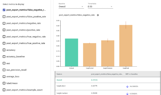
The Fairness Indicators tool suite enables computation and visualization of commonly-identified fairness metrics for classification models, such as false positive rate and false negative rate, making it easy to compare performance across slices or to a baseline slice. The tool computes confidence intervals, which can surface statistically significant disparities, and performs evaluation over multiple thresholds. In the UI, it is possible to toggle the baseline slice and investigate the performance of various other metrics. The user can also add their own metrics for visualization, specific to their use case.

Furthermore, Fairness Indicators is integrated with the What-If Tool (WIT) — clicking on a bar in the Fairness Indicators graph will load those specific data points into the the WIT widget for further inspection, comparison, and counterfactual analysis. This is particularly useful for large datasets, where Fairness Indicators can be used to identify problematic slices before the WIT is used for a deeper analysis.

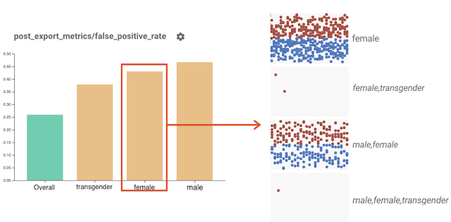
Using Fairness Indicators to visualize metrics for fairness evaluation.
Clicking on a slice in Fairness Indicators will load all the data points in that slice inside the What-If Tool widget. In this case, all data points with the “female” label are shown.

The Fairness Indicators beta launch includes the following:

How To Use Fairness Indicators in Models Today
Fairness Indicators is built on top of TensorFlow Model Analysis, a component of TensorFlow Extended (TFX) that can be used to investigate and visualize model performance. Based on the specific ML workflow, Fairness Indicators can be incorporated into a system in one of the following ways:
If using TensorFlow models and tools, such as TFX:

  • Access Fairness Indicators as part of the Evaluator component in TFX
  • Access Fairness Indicators in TensorBoard when evaluating other real-time metrics

If not using existing TensorFlow tools:

  • Download the Fairness Indicators pip package, and use Tensorflow Model Analysis as a standalone tool

For non-TensorFlow models:

Fairness Indicators Case Study
We created a case study and introductory video that illustrates how Fairness Indicators can be used with a combination of tools to detect and mitigate bias in a model trained on Jigsaw’s Unintended Bias in Toxicity dataset. The dataset was developed by Conversation AI, a team within Jigsaw that works to train ML models to protect voices in conversation. Models are trained to predict whether text comments are likely to be abusive along a variety of dimensions including toxicity, insult, and sexual explicitness.

The primary use case for models such as these is content moderation. If a model penalizes certain types of messages in a systematic way (e.g., often marks comments as toxic when they are not, leading to a high false positive rate), those voices will be silenced. In the case study, we investigated false positive rate on subgroups sliced by gender identity keywords that are present in the dataset, using a combination of tools (Fairness Indicators, TFDV, and WIT) to detect, diagnose, and take steps toward remediating the underlying problem.

What’s next?
Fairness Indicators is only the first step. We plan to expand vertically by enabling more supported metrics, such as metrics that enable you to evaluate classifiers without thresholds, and horizontally by creating remediation libraries that utilize methods, such as active learning and min-diff. Because we believe it is important to learn through real examples, we hope to ground our work in more case studies to be released over the next few months, as more features become available.

To get started, see the Fairness Indicators GitHub repo. For more information on how to think about fairness evaluation in the context of your use case, see this link.

We would love to partner with you to understand where Fairness Indicators is most useful, and where added functionality would be valuable. Please reach out at tfx@tensorflow.org to provide any feedback on your experience!

Acknowledgements
The core team behind this work includes Christina Greer, Manasi Joshi, Huanming Fang, Shivam Jindal, Karan Shukla, Osman Aka, Sanders Kleinfeld, Alicia Chang, Alex Hanna, and Dan Nanas. We would also like to thank James Wexler, Mahima Pushkarna, Meg Mitchell and Ben Hutchinson for their contributions to the project.

Amazon Polly Neural Text-to-Speech voices now available in Sydney Region

Amazon Polly turns text into lifelike speech for voice-enabled applications. AWS is excited to announce the general availability of all Neural Text-to-Speech (NTTS) voices in the Asia Pacific (Sydney) Region. These voices deliver groundbreaking improvements in speech quality through a new machine learning approach. If you are in the Sydney Region, you can now synthesize 13 NTTS voices (eight US English, three UK English, one US Spanish, and one Brazilian Portuguese) available in the Amazon Polly portfolio.

In addition, Amazon Polly’s two speaking style voices are available in US English (Matthew and Joanna). Newscaster simulates the tone of a news anchor, and Conversational simulates the tone of a friendly conversation. Both are built using the same NTTS technology.

Listen to samples of both speaking styles:

Newscaster

Listen now

Voiced by Amazon Polly

Conversational

Listen now

Voiced by Amazon Polly

The entire Amazon Polly portfolio of 60+ voices (Neural and Standard) across 29 languages is now available in the Asia Pacific (Sydney) region. Visit the Amazon Polly documentation for the full list of text-to-speech voices, and log in to the Amazon Polly console to try them out! Simply set the ‘engine‘ parameter to ‘neural‘, and select one of the 4 AWS regions that support NTTS voices.


About the Author

Ankit Dhawan is a Senior Product Manager for Amazon Polly, a technology enthusiast, and a huge Liverpool FC fan. When not working on delighting our customers, you will find him exploring the Pacific Northwest with his wife and dog. He is an eternal optimist, loves reading biographies, and playing poker. You can indulge him in a conversation on technology, entrepreneurship, or soccer anytime of the day.