In this blog post, we explore a functional paradigm for implementing
reinforcement learning
(RL) algorithms. The paradigm will be that developers write the numerics of
their algorithm as independent, pure functions, and then use a library to
compile them into policies that can be trained at scale. We share how these
ideas were implemented in RLlib’s policy builder
API,
eliminating thousands of lines of “glue” code and bringing support for
Keras
and TensorFlow
2.0.

<!–

–>

Why Functional Programming?

One of the key ideas behind functional programming is that programs can be
composed largely of pure functions, i.e., functions whose outputs are entirely
determined by their inputs. Here less is more: by imposing restrictions on what
functions can do, we gain the ability to more easily reason about and
manipulate their execution.

<!–

–>

In TensorFlow, such functions of tensors can be executed either
symbolically with placeholder inputs or eagerly with real tensor
values. Since such functions have no side-effects, they have the same effect on
inputs whether they are called once symbolically or many times eagerly.

Functional Reinforcement Learning

Consider the following loss function over agent rollout data, with current
state $s$, actions $a$, returns $r$, and policy $pi$:

L(s, a, r) = -[log pi(s, a)] cdot r

If you’re not familiar with RL, all this function is saying is that we should
try to improve the probability of good actions (i.e., actions that increase
the future returns). Such a loss is at the core of policy
gradient
algorithms. As we will see, defining the loss is almost all you need to start
training a RL policy in RLlib.

<!–

–>


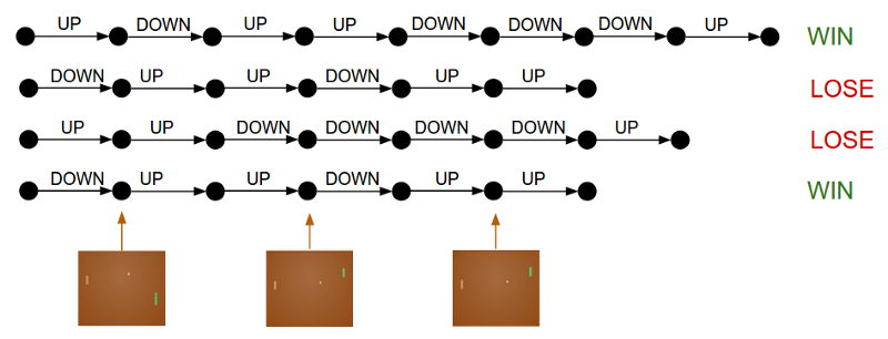
Given a set of rollouts, the policy gradient
loss seeks to improve the probability of good actions (i.e., those that lead to
a win in this Pong example above).

A straightforward translation into Python is as follows. Here, the loss
function takes $(pi, s, a, r)$, computes $pi(s, a)$ as a discrete action
distribution, and returns the log probability of the actions multiplied by the
returns:

def loss(model, s: Tensor, a:  Tensor, r: Tensor) -> Tensor:
    logits = model.forward(s)
    action_dist = Categorical(logits)
    return -tf.reduce_mean(action_dist.logp(a) * r)

There are multiple benefits to this functional definition. First, notice that
loss reads quite naturally — there are no placeholders, control loops, access
of external variables, or class members as commonly seen in RL
implementations. Second, since it doesn’t mutate external state, it is
compatible with both TF graph and eager mode execution.

<!–

–>


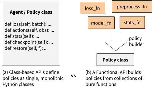
In contrast to a class-based API, in which class methods can access arbitrary
parts of the class state, a functional API builds policies from loosely coupled
pure functions.

In this blog we explore defining RL algorithms as collections of such pure
functions. The paradigm will be that developers write the numerics of their
algorithm as independent, pure functions, and then use a RLlib helper function
to compile them into policies that can be trained at scale. This proposal is
implemented concretely in the RLlib library.

Functional RL with RLlib

RLlib is an open-source
library for reinforcement learning that offers both high scalability and a
unified API for a variety of applications. It offers a wide range of scalable
RL algorithms.

<!–

–>


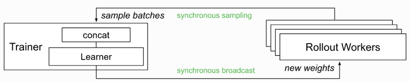
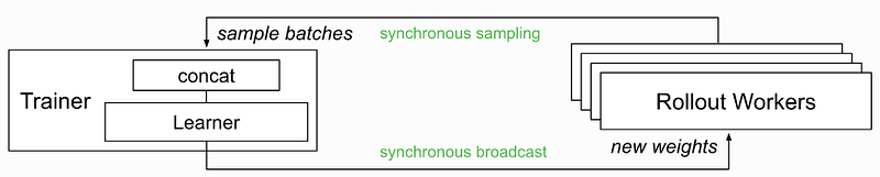
Example of how RLlib scales algorithms, in this case with distributed
synchronous sampling.

Given the increasing popularity of PyTorch (i.e., imperative execution) and the
imminent release of TensorFlow 2.0, we saw the opportunity to improve RLlib’s
developer experience with a functional rewrite of RLlib’s algorithms. The major
goals were to:

Improve the RL debugging experience

• Allow eager execution to be used for any algorithm with just an — eager
  flag, enabling easy print() debugging.

Simplify new algorithm development

• Make algorithms easier to customize and understand by replacing monolithic
  “Agent” classes with policies built from collections of pure functions
  (e.g., primitives provided by TRFL).
• Remove the need to manually declare tensor placeholders for TF.
• Unify the way TF and PyTorch policies are defined.

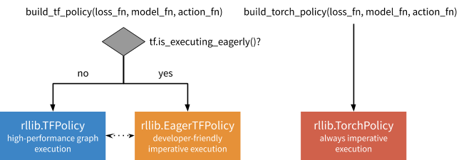
Policy Builder API

The RLlib policy builder API for functional RL (stable in RLlib 0.7.4) involves
just two key functions:

• build_tf_policy()
• build_torch_policy()

At a high level, these builders take a number of function objects as input,
including a loss_fn similar to what you saw earlier, a model_fn to return a
neural network model given the algorithm config, and an action_fn to generate
action samples given model outputs. The actual API takes quite a few more
arguments, but these are the main ones. The builder compiles these functions
into a
policy
that can be queried for actions and improved over time given experiences:

<!–

–>

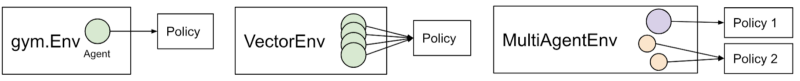
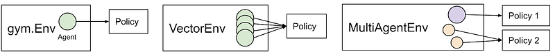
These policies can be leveraged for single-agent, vector, and multi-agent
training in RLlib, which calls on them to determine how to interact with
environments:

<!–

–>

We’ve found the policy builder pattern general enough to port almost all of RLlib’s reference algorithms, including A2C, APPO, DDPG, DQN, PG, PPO, SAC, and IMPALA in TensorFlow, and PG / A2C in PyTorch. While code readability is somewhat subjective, users have reported that the builder pattern makes it much easier to customize algorithms, especially in environments such as Jupyter notebooks. In addition, these refactorings have reduced the size of the algorithms by up to hundreds of lines of code each.

Vanilla Policy Gradients Example

<!–

–>


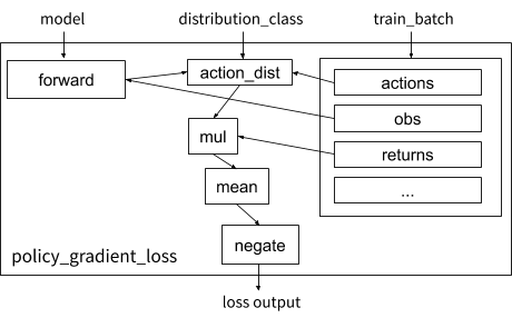
Visualization of the vanilla policy gradient loss function in RLlib.

Let’s take a look at how the earlier loss example can be implemented concretely
using the builder pattern. We define policy_gradient_loss, which requires a
couple of tweaks for generality: (1) RLlib supplies the proper
distribution_class so the algorithm can work with any type of action space
(e.g., continuous or categorical), and (2) the experience data is held in a
train_batch dict that contains state, action, etc. tensors:

def policy_gradient_loss(
        policy, model, distribution_cls, train_batch):
    logits, _ = model.from_batch(train_batch)
    action_dist = distribution_cls(logits, model)
    return -tf.reduce_mean(
        action_dist.logp(train_batch[“actions”]) *
        train_batch[“returns”])

To add the “returns” array to the batch, we need to define a postprocessing
function that calculates it as the temporally discounted
reward
over the trajectory:

R(tau) = sum_{t=0}^{infty}{gamma^tr_t}

We set $gamma = 0.99$ when computing $R(T)$ below in code:

from ray.rllib.evaluation.postprocessing import discount

# Run for each trajectory collected from the environment
def calculate_returns(policy,
                      batch,
                      other_agent_batches=None,
                      episode=None):
   batch[“returns”] = discount(batch[“rewards”], 0.99)
   return batch

Given these functions, we can then build the RLlib policy and
trainer
(which coordinates the overall training workflow). The model and action
distribution are automatically supplied by RLlib if not specified:

MyTFPolicy = build_tf_policy(
   name="MyTFPolicy",
   loss_fn=policy_gradient_loss,
   postprocess_fn=calculate_returns)

MyTrainer = build_trainer(
   name="MyCustomTrainer", default_policy=MyTFPolicy)

Now we can run this at the desired scale using
Tune, in this example showing
a configuration using 128 CPUs and 1 GPU in a cluster:

tune.run(MyTrainer,
    config={“env”: “CartPole-v0”,
            “num_workers”: 128,
            “num_gpus”: 1})

While this example (runnable
code)
is only a basic algorithm, it demonstrates how a functional API can be concise,
readable, and highly scalable. When compared against the previous way to define
policies in RLlib using TF placeholders, the functional API uses ~3x
fewer lines of code (23 vs 81 lines), and also works in eager:

<!–

–>


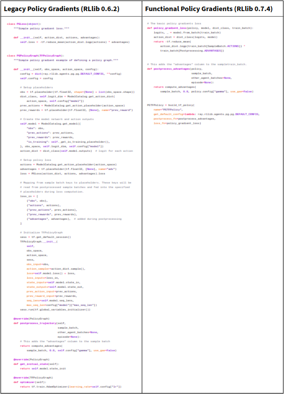
Comparing the legacy class-based API
with the new functional policy builder API
Both policies implement the same behaviour, but the functional definition is
much shorter.

How the Policy Builder works

Under the hood, build_tf_policy takes the supplied building blocks
(model_fn, action_fn, loss_fn, etc.) and compiles them into either a
DynamicTFPolicy
or
EagerTFPolicy,
depending on if TF eager execution is enabled. The former implements graph-mode
execution (auto-defining placeholders dynamically), the latter eager execution.

The main difference between DynamicTFPolicy and EagerTFPolicy is how many
times they call the functions passed in. In either case, a model_fn is
invoked once to create a Model class. However, functions that involve tensor
operations are either called once in graph mode to build a symbolic computation
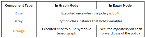
graph, or multiple times in eager mode on actual tensors. In the following
figures we show how these operations work together in blue and orange:

<!–

–>

<!–

–>


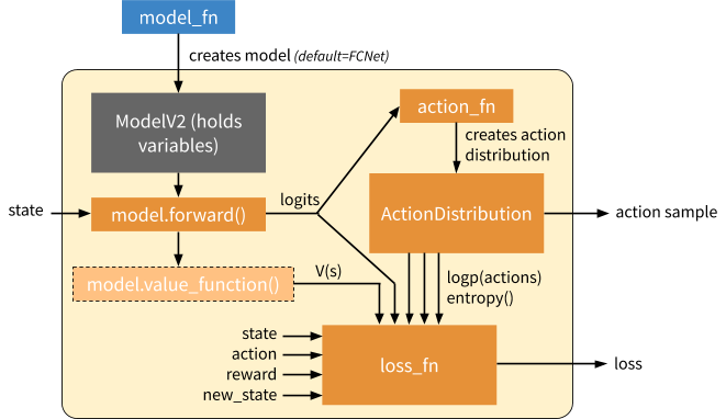
Overview of a generated EagerTFPolicy. The policy passes the environment state
through model.forward(), which emits output logits. The model output
parameterizes a probability distribution over actions (“ActionDistribution”),
which can be used when sampling actions or training. The loss function operates
over batches of experiences. The model can provide additional methods such as a
value function (light orange) or other methods for computing Q values, etc.
(not shown) as needed by the loss function.

This policy object is all RLlib needs to launch and scale RL training.
Intuitively, this is because it encapsulates how to compute actions and improve
the policy. External state such as that of the environment and RNN hidden state
is managed externally by RLlib, and does not need to be part of the policy
definition. The policy object is used in one of two ways depending on whether
we are computing rollouts or trying to improve the policy given a batch of
rollout data:

<!–

–>


Inference: Forward pass to compute a single action. This only involves
querying the model, generating an action distribution, and sampling an action
from that distribution. In eager mode, this involves calling action_fn

DQN example of an action sampler,
which creates an action distribution / action sampler as relevant that is then
sampled from.

<!–

–>


Training: Forward and backward pass to learn on a batch of experiences.
In this mode, we call the loss function to generate a scalar output which can
be used to optimize the model variables via SGD. In eager mode, both action_fn
and loss_fn are called to generate the action distribution and policy loss
respectively. Note that here we don’t show differentiation through action_fn,
but this does happen in algorithms such as DQN.

Loose Ends: State Management

RL training inherently involves a lot of state. If algorithms are defined using
pure functions, where is the state held? In most cases it can be managed
automatically by the framework. There are three types of state that need to be
managed in RLlib:

1. Environment state: this includes the current state of the environment
   and any recurrent state passed between policy steps. RLlib manages this
   internally in its rollout
   worker
   implementation.
2. Model state: these are the policy parameters we are trying to learn via
   an RL loss. These variables must be accessible and optimized in the same way
   for both graph and eager mode. Fortunately,
   Keras models can be used in either
   mode. RLlib provides a customizable model class
   (TFModelV2)
   based on the object-oriented Keras style to hold policy parameters.
3. Training workflow state: state for managing training, e.g., the
   annealing schedule for various hyperparameters, steps since last update, and so
   on. RLlib lets algorithm authors add mixin
   classes
   to policies that can hold any such extra variables.

Loose ends: Eager Overhead

Next we investigate RLlib’s eager mode performance with eager
tracing on or
off. As shown in the below figure, tracing greatly improves performance.
However, the tradeoff is that Python operations such as print may not be called
each time. For this reason, tracing is off by default in RLlib, but can be
enabled with “eager_tracing”: True. In addition, you can also set
“no_eager_on_workers” to enable eager only for learning but disable it for
inference:

<!–

–>

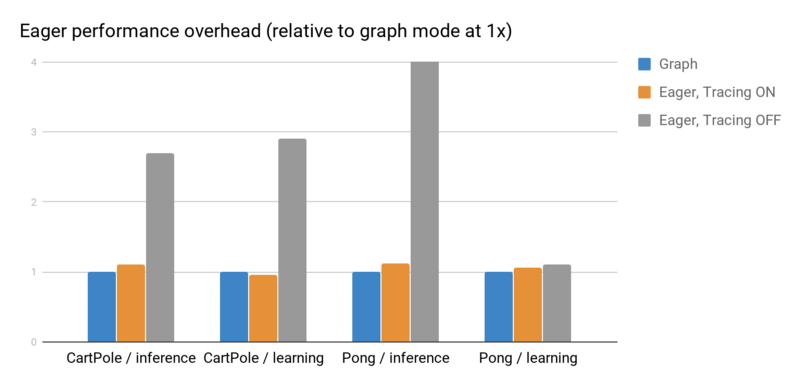
Eager inference and gradient overheads measured using rllib train --run=PG
--env=<env> [ --eager [ --trace]] on a laptop processor. With tracing off, eager
imposes a significant overhead for small batch operations. However it is often
as fast or faster than graph mode when tracing is enabled.

Conclusion

To recap, in this blog post we propose using ideas from functional programming
to simplify the development of RL algorithms. We implement and validate these
ideas in RLlib. Beyond making it easy to support new features such as eager
execution, we also find the functional paradigm leads to substantially more
concise and understandable code. Try it out yourself with pip install
ray[rllib] or by checking out the
docs and source
code.

If you’re interested in helping improve RLlib, we’re also hiring.