Kinect Energy uses Amazon SageMaker to Forecast energy prices with Machine Learning
The Amazon ML Solutions Lab worked with Kinect Energy recently to build a pipeline to predict future energy prices based on machine learning (ML). We created an automated data ingestion and inference pipeline using Amazon SageMaker and AWS Step Functions to automate and schedule energy price prediction.
The process makes special use of the Amazon SageMaker DeepAR forecasting algorithm. By using a deep learning forecasting model to replace the current manual process, we saved Kinect Energy time and put a consistent, data-driven methodology into place.
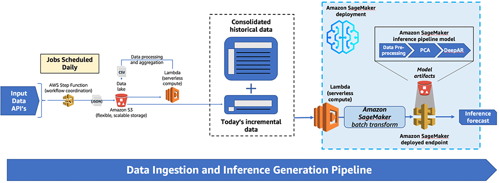
The following diagram shows the end-to-end solution.

The data ingestion is orchestrated using a step function which loads and processes data daily and deposits it is into a data lake in Amazon S3. The data is then passed to Amazon SageMaker which handles inference generation via a batch transform call that triggers an inference pipeline model.
Project motivation
The natural power market depends on a range of sources for production—wind, hydro-reservoir generation, nuclear, coal, and oil & gas—to meet consumer demand. The actual mix of power sources used to satisfy that demand depends on the price of each energy component on a given day. That price depends on that day’s power demand. Investors then trade the price of electricity in an open market.
Kinect Energy buys and sells energy to clients, and an important piece of their business model involves trading financial contracts derived from energy prices. This requires an accurate forecast of the energy price.
Kinect Energy wanted to improve and automate the process of forecasting—historically done manually—by using ML. The spot price is the current commodity price, as opposed to the future or forward price—the price at which a commodity can be bought or sold for future delivery. Comparing predicted spot prices and forward prices provides opportunities for the Kinect Energy team to hedge against future price movements based on current predictions.
Data requirements
In this solution, we wanted to predict spot prices for a four-week outlook on an hourly interval. One of the major challenges for the project involved creating a system to gather and process the required data automatically. The pipeline required two main components of the data:
- Historic spot prices
- Energy production and consumption rates and other external factors that influence the spot price
(We denote the production and consumption rates as external data.)
To build a robust forecasting model, we had to gather enough historical data to train the model, preferably spanning multiple years. We also had to update the data daily as the market generates new information. The model also needed access to a forecast of the external data components for the entire period over which the model forecasts.
Vendors update hourly spot prices to an external data feed daily. Various other entities provide data components on production and consumption rates, publishing their data on different schedules.
The analysts of the Kinect Energy team require the spot price forecast at a specific time of the day to shape their trading strategy. So, we had to build a robust data pipeline that periodically calls multiple API actions. Those actions collect data, perform the necessary preprocessing, and then store it in an Amazon S3 data lake where the forecasting model accesses it.
The data ingestion and inference generation pipeline
The pipeline consists of three main steps orchestrated by an AWS Step Function state machine: data ingestion, data storage, and inference generation. An Amazon CloudWatch event triggers the state machine to run on a daily schedule to prepare the consumable data.

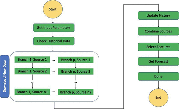
The flowchart above details the individual steps that consist of the entire step function. The step function coordinates downloading of new data, updating of the historical data, and generating new inferences so that the whole process can be carried out in a single continuous workflow.
Although we built the state machine around a daily schedule, it employs two modes of data retrieval. By default, the state machine downloads data daily. A user can manually trigger the process to download the full historical data on demand as well for setup or recovery. The step function calls multiple API actions to gather the data, each with different latencies. The data gathering processes run in parallel. This step also performs all the required preprocessing, and stores the data in S3 organized by time-stamped prefixes.
The next step updates the historical data for each component by appending the respective daily elements. Additional processing prepares it in the format that DeepAR requires and sends the data to another designated folder.
The model then triggers an Amazon SageMaker batch transform job that pulls the data from that location, generates the forecast, and finally stores the result in another time-stamped folder. An Amazon QuickSight dashboard picks up the forecast and displays it to the analysts.
Packaging required dependencies into AWS Lambda functions
We set up Python pandas and the scikit-learn (sklearn) library to handle most of the data preprocessing. These libraries aren’t available by default for import into a Lambda function that Step Function calls. To adapt, we packaged the Lambda function Python script and its necessary imports into a .zip file.
This additional code uploads the .zip file to the target Lambda function:
Exception handling
One of the common challenges of writing robust production code is anticipating possible failure mechanisms and mitigating them. Without instructions to handle unusual events, the pipeline can fall apart.
Our pipeline presents two major potentials for failure. First, our data ingestion relies on external API data feeds, which could experience downtime, leading our queries to fail. In this case, we set a fixed number of retry attempts before the process marks the data feed temporarily unavailable. Second, feeds may not provide updated data and instead return old information. In this case, the API actions do not return errors, so our process needs the ability to decide for itself if the information is new.
Step Functions provide a retry option to automate the process. Depending on the nature of the exception, we can set the interval between two successive attempts (IntervalSeconds) and the maximum number of times to try the action (MaxAttempts). The parameter BackoffRate=1 arranges the attempts at a regular interval, whereas BackoffRate=2 means every interval is twice the length of the previous one.
Flexibility in data retrieval modes
We built the Step Function state machine to provide functionality for two distinct data retrieval modes:
- A historical data pull to grab the entire existing history of the data
- A refreshed data pull to grab the incremental daily data
The Step Function normally only has to extract the historical data one time in the beginning and store it in the S3 data lake. The stored data grows as the state machine appends new daily data. The option to refresh the historical data exists by setting the parameter full_history_download to True in the Lambda function that the CheckHistoricalData step calls. Doing so refreshes the entire dataset.
Building the forecasting model
We built the ML model in Amazon SageMaker. After putting together a collection of historical data on S3, we cleaned and prepared it using popular Python libraries such as pandas and sklearn.
A separate Amazon SageMaker ML algorithm called principal component analysis (PCA) was used to perform the feature engineering. To reduce the scope of our feature space while preserving information and creating desirable features, we applied PCA to our dataset before training our forecasting model.
We used a separate Amazon SageMaker ML algorithm called DeepAR as the forecasting model. DeepAR is a custom forecasting algorithm that specializes in processing time-series data. Amazon originally used the algorithm for product demand forecasting. Its ability to predict consumer demand based on temporal data and various external factors made the algorithm a strong choice to predict the fluctuations in energy price based on usage.
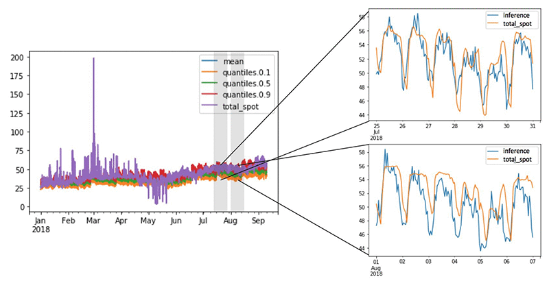
The following figure demonstrates some modelling results. We tested the model on available 2018 data after training it on historical data. A benefit of using the DeepAR model is that it returns a confidence interval from 10%-90%, providing a forecasted range. Zooming in to different time periods of the forecast, we can see that DeepAR excels at reproducing past periodic temporal patterns compared to the actual price records.

Above shows a comparison between values predicted by the DeepAR model versus the actual values over the test set of January to September 2018.
Amazon SageMaker also provides a straightforward way to perform hyperparameter optimization (HPO). After model training, we tuned the hyperparameters of the model to extract incrementally better model performance. Amazon SageMaker HPO uses Bayesian optimization to search the hyperparameter space and identify the ideal parameters for different models.
The Amazon SageMaker HPO API makes it simple to specify resource constraints such as the number of training jobs and computing power allocated to the process. We chose to test ranges for common parameters important to the DeepAR structure, such as the dropout rate, embedding dimension, and the number of layers in the neural network.
Packaging modeling steps into an Amazon SageMaker inference pipeline with sklearn containers
To implement and deploy an ML model effectively, we had to ensure that the data input format and processing from the inference matched up with the format and processing used for model training.
Our model pipeline uses sklearn functions for data processing and transformations, as well as a PCA feature engineering step before training using DeepAR. To preserve this process in an automated pipeline, we used prebuilt sklearn containers within Amazon SageMaker and the Amazon SageMaker inference pipelines model.
Within the Amazon SageMaker SDK, a set of sklearn classes handles end-to-end training and deployment of custom sklearn code. For example, the following code shows a sklearn Estimator executing an sklearn script in a managed environment. The managed sklearn environment is an Amazon Docker container that executes functions defined in the entry_point Python script. We supplied the preprocessing script as a .py file path. After fitting the Amazon SageMaker sklearn model on the training data, we can ensure that the same pre-fit model processes the data at inference time.
After this, we strung together the modeling sequence using Amazon SageMaker inference pipelines. The PipelineModel class within the Amazon SageMaker SDK creates an Amazon SageMaker model with a linear sequence of two to five containers to process requests for data inferences. With this, we can define and deploy any combination of trained Amazon SageMaker algorithms or custom algorithms packaged in Docker containers.
Like other Amazon SageMaker model endpoints, the process handles pipeline model invocations as a sequence of HTTP requests. The first container in the pipeline handles the initial request, and then the second container handles the intermediate response, and so on. The last container in the pipeline eventually returns the final response to the client.
A crucial consideration when constructing a PipelineModel is to note the data formatting for both the input and output for each container. For example, the DeepAR model requires a specific data structure for input data during training and a JSON Lines data format for inference. This format is different from supervised ML models because a forecasting model requires additional metadata, such as the starting date and the time interval of the time-series data.
After creation, using a pipeline model provided the benefit of a single endpoint that could handle inference generation. Besides ensuring that preprocessing on training data matched that at inference time, we can deploy a single endpoint that runs the entire workflow from data input to inference generation.
Model deployment using batch transform
We used Amazon SageMaker batch transform to handle inference generation. You can deploy a model in Amazon SageMaker in one of two ways:
- Create a persistent HTTPS endpoint where the model provides real-time inference.
- Run an Amazon SageMaker batch transform job that starts an endpoint, generates inferences on the stored dataset, outputs the inference predictions, and then shuts down the endpoint.
Due to the specifications of this energy forecasting project, the batch transform technique proved the better choice. Instead of real-time predictions, Kinect Energy wanted to schedule daily data collection and forecasting, and use this output for their trading analysis. With this solution, Amazon SageMaker takes care of starting up, managing, and shutting down the required resources.
DeepAR best practices suggest that the entire historical time-series for the target and dynamic features should be provided to the model at both training and inference. This is because the model uses data points further back to generate lagged features and input datasets can grow very large.
To avoid the usual 5-MB request body limit, we created a batch transform using the inference pipeline model and set the limit for input data size using the max_payload argument. Then, we generated input data using the same function we used on the training data and added it to an S3 folder. We could then point the batch transform job to this location and generate an inference on that input data.
Automating inference generation
Finally, we created a Lambda function that generates daily forecasts. To do this, we converted the code to the Boto3 API so Lambda can use it.
The Amazon SageMaker SDK library lets us access and invoke the trained ML models, but is far larger than the 50-MB limit for including in a Lambda function. Instead, we used the natively-available Boto3 library.
Conclusion
Along with the Kinect Energy team, we were able to create an automated data ingestion and inference generation pipeline. We used AWS Lambda and AWS Step Functions to automate and schedule the entire process.
In the Amazon SageMaker platform, we built, trained, and tested a DeepAR forecasting model to predict electricity spot prices. Amazon SageMaker inference pipelines combined preprocessing, feature engineering, and model output steps. A single Amazon SageMaker batch transform job could put the model into production and generate an inference. These inferences now help Kinect Energy make more accurate predictions of spot prices and improve their electricity price trading capabilities.
The Amazon ML Solutions Lab engagement model provided the opportunity to deliver a production-ready ML model. It also gave us the chance to train the Kinect Energy team on data science practices so that they can maintain, iterate, and improve upon their ML efforts. With the resources provided, they can expand to other possible future use cases.
Get started today! You can learn more about Amazon SageMaker and kickoff your own Machine Learning solution by visiting the Amazon SageMaker console.
About the Authors
 Han Man is a Data Scientist with AWS Professional Services. He has a PhD in engineering from Northwestern University and has several years of experience as a management consultant advising clients across many industries. Today he is passionately working with customers to develop and implement machine learning, deep learning, & AI solutions on AWS. He enjoys playing basketball in his spare time and taking his bulldog, Truffle, to the beach.
 Arkajyoti Misra is a Data Scientist working in AWS Professional Services. He loves to dig into Machine Learning algorithms and enjoys reading about new frontiers in Deep Learning.
 Matt McKenna is a Data Scientist focused on machine learning in Amazon Alexa, and is passionate about applying statistics and machine learning methods to solve real world problems. In his spare time, Matt enjoys playing guitar, running, craft beer, and rooting for Boston sports teams.
Many thanks to Kinect Energy team who worked on the project. Special thanks to following leaders from Kinect Energy who encouraged and reviewed the blog post.
- Tulasi Beesabathuni: Tulasi is the squad lead for both Artificial Intelligence / Machine Learning and Box / OCR (content management) at World Fuel Services. Tulasi oversaw the initiation, development and deployment of the Power Prediction Model and employed his technical and leadership skillsets to complete the team’s first use case using new technology.
- Andrew Stypa: Andrew is the lead business analyst for the Artificial Intelligence / Machine learning squad at World Fuel Services. Andrew used his prior experiences in the business to initiate the use case and ensure that the trading team’s specifications were met by the development team.