Interpretation for Text Classification

Last week, I gave a talk on “Hands-on Feature Engineering for NLP” at QCon New York. As a very small part of the presentation, I gave a brief demo on how LIME & SHAP work in terms of text classification explainability.

I decided to write a blog post about them because they are fun, easy to use and visually compelling.

All machine learning models that operate in higher dimensions than what can be directly visualized by the human mind can be referred as black box models which come down to the interpretability of the models. In particular in the field of NLP, it’s always the case that the dimension of the features are very huge, explaining feature importance is getting much more complicated.

LIME & SHAP help us provide an explanation not only to end users but also ourselves about how a NLP model works.

Using the Stack Overflow questions tags classification data set, we are going to build a multi-class text classification model, then applying LIME & SHAP separately to explain the model. Because we have done text classification many times before, we will quickly build the NLP models and focus on the models interpretability.

Data Pre-processing, Feature Engineering and Logistic Regression

Our objective here is not to produce the highest results. I wanted to dive into LIME & SHAP as soon as possible and that’s what happened next.

Interpreting text predictions with LIME

From now on, it’s the fun part. The following code snippets were largely borrowed from LIME tutorial.

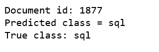
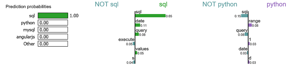
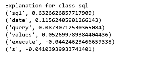
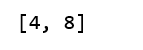
We randomly select a document in test set, it happens to be a document that labeled as sql, and our model predicts it as sql as well. Using this document, we generate explanations for label 4 which is sql and label 8 which is python.

print ('Explanation for class %s' % class_names[4])
print ('n'.join(map(str, exp.as_list(label=4))))

print ('Explanation for class %s' % class_names[8])
print ('n'.join(map(str, exp.as_list(label=8))))

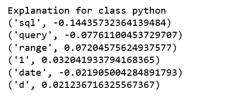
It is obvious that this document has the highest explanation for label sql. We also notice that the positive and negative signs are with respect to a particular label, such as word “sql” is positive towards class sql while negative towards class python, and vice versa.

We are going to generate labels for the top 2 classes for this document.

exp = explainer.explain_instance(X_test[idx], c.predict_proba, num_features=6, top_labels=2)
print(exp.available_labels())

It gives us sql and python.

exp.show_in_notebook(text=False)

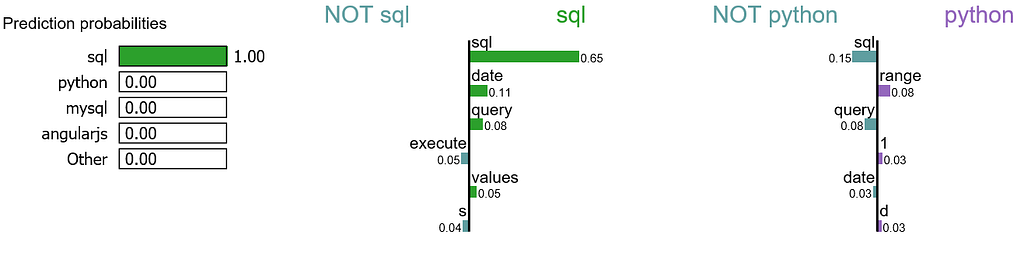
Let me try to explain this visualization:

• For this document, word “sql” has the highest positive score for class sql.
• Our model predicts this document should be labeled as sql with the probability of 100%.
• If we remove word “sql” from the document, we would expect the model to predict label sql with the probability at 100% — 65% = 35%.
• On the other hand, word “sql” is negative for class python, and our model has learned that word “range” has a small positive score for class python.

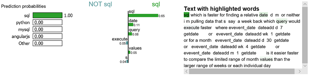
We may want to zoom in and study the explanations for class sql, as well as the document itself.

exp.show_in_notebook(text=y_test[idx], labels=(4,))

Interpreting text predictions with SHAP

The following process were learned from this tutorial.

• After model is trained, we use the first 200 training documents as our background data set to integrate over, and to create a SHAP explainer object.
• We get the attribution values for individual predictions on a subset of the test set.
• Transform the index to words.
• Use SHAP’s summary_plot method to show the top features impacting model predictions.

attrib_data = X_train[:200]
explainer = shap.DeepExplainer(model, attrib_data)
num_explanations = 20
shap_vals = explainer.shap_values(X_test[:num_explanations])

words = processor._tokenizer.word_index
word_lookup = list()
for i in words.keys():
  word_lookup.append(i)

word_lookup = [''] + word_lookup
shap.summary_plot(shap_vals, feature_names=word_lookup, class_names=tag_encoder.classes_)

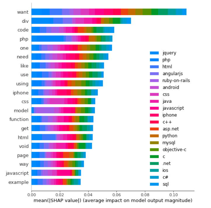
• Word “want” is the biggest signal word used by our model, contribute most to class jquery predictions.
• Word “php” is the 4th biggest signal word used by our model, contributing most to class php of course.
• On the other hand, word “php” is likely to have a negative signal to the other class because it is unlikely to see word “php” to appear in a python document.

There are a lot to learn in terms of machine learning interpretability with LIME & SHAP. I have only covered a tiny piece for NLP. Jupyter notebook can be found on Github. Enjoy the fun!

Explain NLP models with LIME & SHAP was originally published in Towards Data Science on Medium, where people are continuing the conversation by highlighting and responding to this story.