Blog

Learn About Our Meetup

5000+ Members

MEETUPS

LEARN, CONNECT, SHARE

Join our meetup, learn, connect, share, and get to know your Toronto AI community. 

JOB POSTINGS

INDEED POSTINGS

Browse through the latest deep learning, ai, machine learning postings from Indeed for the GTA.

CONTACT

CONNECT WITH US

Are you looking to sponsor space, be a speaker, or volunteer, feel free to give us a shout.

Author: torontoai

Top Shot on Pixel 3

Life is full of meaningful moments — from a child’s first step to an impromptu jump for joy — that one wishes could be preserved with a picture. However, because these moments are often unpredictable, missing that perfect shot is a frustrating problem that smartphone camera users face daily. Using our experience from developing Google Clips, we wondered if we could develop new techniques for the Pixel 3 camera that would allow everyone to capture the perfect shot every time.

Top Shot is a new feature recently launched with Pixel 3 that helps you to capture precious moments precisely and automatically at the press of the shutter button. Top Shot saves and analyzes the image frames before and after the shutter press on the device in real-time using computer vision techniques, and recommends several alternative high-quality HDR+ photos.

Examples of Top Shot on Pixel 3. On the left, a better smiling shot is recommended. On the right, a better jump shot is recommended. The recommended images are high-quality HDR+ shots.

Capturing Multiple Moments
When a user opens the Pixel 3 Camera app, Top Shot is enabled by default, helping to capture the perfect moment by analyzing images taken both before and after the shutter press. Each image is analyzed for some qualitative features (e.g., whether the subject is smiling or not) in real-time and entirely on-device to preserve privacy and minimize latency. Each image is also associated with additional signals, such as optical flow of the image, exposure time, and gyro sensor data to form the input features used to score the frame quality.

When you press the shutter button, Top Shot captures up to 90 images from 1.5 seconds before and after the shutter press, selecting up to two alternative shots to save in high resolution — the original shutter frame and high-res alternatives for you to review (other lower-res frames can also be reviewed as desired). The shutter frame is processed and saved first. The best alternative shots are saved afterwards. Google’s Visual Core on Pixel 3 is used to process these top alternative shots as HDR+ images with a very small amount of extra latency, and are embedded into the file of the Motion Photo.

Top-level diagram of Top Shot capture.

Given Top Shot runs in the camera as a background process, it must have very low power consumption. As such, Top Shot uses a hardware-accelerated MobileNet-based single shot detector (SSD). The execution of such optimized models is also throttled by power and thermal limits.

Recognizing Top Moments
When we set out to understand how to enable people to capture the best moments with their camera, we focused on three key attributes: 1) functional qualities like lighting, 2) objective attributes (are the subject’s eyes open? Are they smiling?), and 3) subjective qualities like emotional expressions. We designed a computer vision model to recognize these attributes while operating in a low-latency, on-device mode.

During our development process, we started with a vanilla MobileNet model and set out to optimize for Top Shot, arriving at a customized architecture that operated within our accuracy, latency and power tradeoff constraints. Our neural network design detects low-level visual attributes in early layers, like whether the subject is blurry, and then dedicates additional compute and parameters toward more complex objective attributes like whether the subject’s eyes are open, and subjective attributes like whether there is an emotional expression of amusement or surprise. We trained our model using knowledge distillation over a large number of diverse face images using quantization during both training and inference.

We then adopted a layered Generalized Additive Model (GAM) to provide quality scores for faces and combine them into a weighted-average “frame faces” score. This model made it easy for us to interpret and identify the exact causes of success or failure, enabling rapid iteration to improve the quality and performance of our attributes model. The number of free parameters was on the order of dozens, so we could optimize these using Google’s black box optimizer, Vizier, in tandem with any other parameters that affected selection quality.

Frame Scoring Model
While Top Shot prioritizes for face analysis, there are good moments in which faces are not the primary subject. To handle those use cases, we include the following additional scores in the overall frame quality score:

  • Subject motion saliency score — the low-resolution optical flow between the current frame and the previous frame is estimated in ISP to determine if there is salient object motion in the scene.
  • Global motion blur score — estimated from the camera motion and the exposure time. The camera motion is calculated from sensor data from the gyroscope and OIS (optical image stabilization).
  • “3A” scores — the status of auto exposure, auto focus, and auto white balance, are also considered.

All the individual scores are used to train a model predicting an overall quality score, which matches the frame preference of human raters, to maximize end-to-end product quality.

End-to-End Quality and Fairness
Most of the above components are each evaluated for accuracy independently However, Top Shot presents requirements that are uniquely challenging since it’s running real-time in the Pixel Camera. Additionally, we needed to ensure that all these signals are combined in a system with favorable results. That means we need to gauge our predictions against what our users perceive as the “top shot.”

To test this, we collected data from hundreds of volunteers, along with their opinions of which frames (out of up to 90!) looked best. This donated dataset covers many typical use cases, e.g. portraits, selfies, actions, landscapes, etc.

Many of the 3-second clips provided by Top Shot had more than one good shot, so it was important for us to engineer our quality metrics to handle this. We used some modified versions of traditional Precision and Recall, some classic ranking metrics (such as Mean Reciprocal Rank), and a few others that were designed specifically for the Top Shot task as our objective. In addition to these metrics, we additionally investigated causes of image quality issues we saw during development, leading to improvements in avoiding blur, handling multiple faces better, and more. In doing so, we were able to steer the model towards a set of selections people were likely to rate highly.

Importantly, we tested the Top Shot system for fairness to make sure that our product can offer a consistent experience to a very wide range of users. We evaluated the accuracy of each signal used in Top Shot on several different subgroups of people (based on gender, age, ethnicity, etc), testing for accuracy of each signal across those subgroups.

Conclusion
Top Shot is just one example of how Google leverages optimized hardware and cutting-edge machine learning to provide useful tools and services. We hope you’ll find this feature useful, and we’re committed to further improving the capabilities of mobile phone photography!

Acknowledgements
This post reflects the work of a large group of Google engineers, research scientists, and others including: Ari Gilder, Aseem Agarwala, Brendan Jou, Chris Breithaupt, David Karam, Eric Penner, Farooq Ahmad, Henri Astre, Hillary Strickland, John Zhang, Marius Renn, Matt Bridges, Maxwell Collins, Navid Shiee, Ryan Gordon, Sarah Clinckemaillie, Shu Zhang, Vivek Kesarwani, Xuhui Jia, Yukun Zhu and Yuzo Watanabe.

Amazon SageMaker adds Scikit-Learn support

Amazon SageMaker now comes pre-configured with the Scikit-Learn machine learning library in a Docker container. Scikit-Learn is popular choice for data scientists and developers because it provides efficient tools for data analysis and high quality implementations of popular machine learning algorithms through a consistent Python interface and well documented APIs. Scikit-Learn executes quickly and can scale to most data sets and problems, making it an ideal choice when you need to iterate quickly on your machine learning problems. Unlike Deep Learning frameworks such as TensorFlow or MxNet, Scikit-Learn is used for machine learning and data analysis. You can select from a range of supervised and unsupervised learning algorithms for clustering, regression, classification, dimensionality reduction, feature preprocessing, and model selection.

The newly added Scikit-Learn library is available in the Amazon SageMaker Python SDK. You can write your Scikit-Learn script and use the Amazon SageMaker training capabilities, including automatic model tuning. Once your model is trained, you can deploy your Scikit-Learn models to highly available endpoints that auto-scale to make real-time predictions with low latency. You can also use the same models in large-scale batch transform jobs.

In this blog post, I show you how to use the pre-built Scikit-Learn library in Amazon SageMaker to build, train, and deploy a multi-class classification model.

Training and deploying a Scikit-Learn model

In this example, we’re going to train a decision tree classifier on the IRIS dataset. This example is based on the Scikit-Learn Decision Tree Classification example. The full Amazon SageMaker notebook is available to try out. We’ll highlight the most important pieces here. This dataset has 50 samples from three different species of Iris flower, and is commonly used to demonstrate machine learning techniques. The goal is to predict which of the three species a flower belongs to, based on a number of different properties (petal length, petal width, and so on). While we’re using decision trees to solve this problem, Scikit-Learn offers a number of other algorithms that you can use.

Entry point script

The first step is to write the Scikit-Learn script. Starting with the main guard, we use a parser to read the hyperparameters that we pass to our Amazon SageMaker Estimator when creating the training job. These hyperparameters are made available as arguments to our input script in the training container. In this example, we look for the maximum number of leaf nodes. We also parse a number of Amazon SageMaker-specific environment variables to get information about the training environment, such as the location of input data and location where we want to save the model.

if __name__ == '__main__':
    parser = argparse.ArgumentParser()

    # Hyperparameters are described here. In this simple example we are just including one hyperparameter.
    parser.add_argument('--max_leaf_nodes', type=int, default=-1)

    # SageMaker specific arguments. Defaults are set in the environment variables.
    parser.add_argument('--output-data-dir', type=str, default=os.environ['SM_OUTPUT_DATA_DIR'])
    parser.add_argument('--model-dir', type=str, default=os.environ['SM_MODEL_DIR'])
    parser.add_argument('--train', type=str, default=os.environ['SM_CHANNEL_TRAIN'])

    args = parser.parse_args()

After we’ve defined our hyperparameters, we then load the dataset. For this example, we load all of the CSV files using the Pandas library.

    # Take the set of files and read them all into a single pandas dataframe
    input_files = [ os.path.join(args.train, file) for file in os.listdir(args.train) ]
    if len(input_files) == 0:
        raise ValueError(('There are no files in {}.n' +
                          'This usually indicates that the channel ({}) was incorrectly specified,n' +
                          'the data specification in S3 was incorrectly specified or the role specifiedn' +
                          'does not have permission to access the data.').format(args.train, "train"))
    raw_data = [ pd.read_csv(file, header=None, engine="python") for file in input_files ]
    train_data = pd.concat(raw_data)

In this example, we assume that the label (which species the flower belongs to) is stored in the first column. We separate our features and the label into two separate data frames.

    # labels are in the first column
    train_y = train_data.ix[:,0]
    train_X = train_data.ix[:,1:]

Now we’re ready to train our model. This is as simple as creating the right classifier and calling fit. A key benefit of Scikit-Learn is the simplicity and consistency of the interface that each algorithm exposes. If your model needs pre-processing of features or calculation of validation scoresc, you can also do those things in this step.

    # We determine the number of leaf nodes using the hyper-parameter above.
    max_leaf_nodes = args.max_leaf_nodes

    # Now use scikit-learn's decision tree classifier to train the model.
    clf = tree.DecisionTreeClassifier(max_leaf_nodes=max_leaf_nodes)
    clf = clf.fit(train_X, train_y)

Finally, we save our model.

    # Save the decision tree model.
    joblib.dump(clf, os.path.join(args.model_dir, "model.joblib"))

Amazon SageMaker notebook – Setup

Now that we’ve written our Scikit-Learn script we can run it on Amazon SageMaker using the Amazon SageMaker pre-built Scikit-Learn container. We’re going to use a hosted Jupyter notebook to orchestrate the training process. Feel free to follow along interactively by running the notebook.

First, we set up the Amazon S3 bucket for storing the data and the model, as well as the AWS Identity and Access Management (IAM) role for the data and Amazon SageMaker permissions.

import sagemaker

# S3 prefix
prefix = 'scikit-iris'

# Get a SageMaker-compatible role used by this Notebook Instance.
role = sagemaker.get_execution_role()

Now we’ll import the Python libraries we’ll need and create an Amazon SageMaker session.

from sagemaker.sklearn.estimator import SKLearn

sagemaker_session = sagemaker.Session()

Next, we’ll download our dataset and upload it to Amazon S3. In this example, we use Scikit-Learn locally in our notebook since it provides convenience functions to download the IRIS dataset.

import numpy as np
import os
from sklearn import datasets

# Load Iris dataset, then join labels and features together
iris = datasets.load_iris()
joined_iris = np.insert(iris.data, 0, iris.target, axis=1)


# Create a temporary directory and write the dataset as CSV
os.makedirs('./data', exist_ok=True)
np.savetxt('./data/iris.csv', joined_iris, delimiter=',', fmt='%1.1f, %1.3f, %1.3f, %1.3f, %1.3f')

# Upload the dataset to S3.
train_input = sagemaker_session.upload_data('data', key_prefix="{}/{}".format(prefix, 'data'))

Amazon SageMaker notebook – Training

Now that we’ve prepared the training data and our Scikit-Learn script (which we’ll name scikit_learn_iris.py), the SKLearn class in the SageMaker Python SDK allows us to run that script as a training job on the Amazon SageMaker managed training infrastructure. We’ll also pass the estimator our IAM role, the type of instance we want to use, and a dictionary of the hyperparameters that we want to pass to our script. Since Scikit-Learn runs on a single CPU-only machine, the Estimator only supports an instance count for training of 1 and GPU instances are not supported.

sklearn = SKLearn(
    entry_point='scikit_learn_iris.py',
    train_instance_type="ml.c4.xlarge",
    role=role,
    sagemaker_session=sagemaker_session,
    hyperparameters={'max_leaf_nodes': 30})

After we’ve constructed our SKLearn estimator, we can fit it by passing in the data we uploaded to Amazon S3. Amazon SageMaker makes sure our data is available in the local filesystem of the training cluster, so our Scikit-Learn script can simply read the data from disk.

sklearn.fit({'train': train_input})

Amazon SageMaker Notebook – Deployment

After training, we can use the SKLearn estimator to create an Amazon SageMaker endpoint – a hosted and managed prediction service that we can use to perform inference.

To do this our scikit_learn_iris.py script needs a model_fn() function that loads our saved model to make predictions.

def model_fn(model_dir):
    clf = joblib.load(os.path.join(model_dir, "model.joblib"))
    return clf

You can also optionally specify other functions to customize the behavior of deserialization of the input request (input_fn()), serialization of the predictions (output_fn()), and how predictions are made (predict_fn()). The defaults work for our current use-case so we don’t need to define them.

For more details on the default implementations to customize the behavior, see the SageMaker Scikit-Learn Container GitHub Repository.

Now we can use our SKLearn estimator in the notebook to deploy the model. The deploy() function allows us to set the number and type of instances that will be used for the prediction endpoint. These do not need to be the same values we used for the training job. Here we will deploy the model to a single ml.m4.xlarge instance but you can also deploy the model to more than one instance and set up Auto Scaling for the endpoint.

predictor = sklearn.deploy(initial_instance_count=1, instance_type="ml.m4.xlarge")

Amazon SageMaker notebook – Prediction and evaluation

Now we can use this predictor to classify flowers from the IRIS dataset. Ideally, the evaluation dataset should be different from the training dataset but for this example, we’ll just reuse some of the training dataset to invoke the endpoint. .

First, we create a test dataset.

import itertools
import pandas as pd

shape = pd.read_csv("data/iris.csv", header=None)

a = [50*i for i in range(3)]
b = [40+i for i in range(10)]
indices = [i+j for i,j in itertools.product(a,b)]

test_data = shape.iloc[indices[:-1]]
test_X = test_data.iloc[:,1:]
test_y = test_data.iloc[:,0]

Now we can use the endpoint to make predictions by calling the predict function with our features.

predictor.predict(test_X.values)

Amazon SageMaker notebook – Cleanup

After you have finished with this example, remember to delete the prediction endpoint to release the instances associated with it.

sklearn.delete_endpoint()

Amazon SageMaker notebook – Batch Transform

Amazon SageMaker also provides Batch Transform, a managed service for doing large-scale that can be used to perform inference against your trained model on a large dataset. It’s ideal for scenarios where you’re dealing with large batches of data, you don’t need sub-second latency, or you need to preprocess and transform the training data.

First, we create a transformer and specify the number and type of instances we want to use for the job. In this case we specify 2 instances but you can scale this with the size of your dataset to reduce the amount of time it takes.

# Define a SKLearn Transformer from the trained SKLearn Estimator
transformer = sklearn.transformer(instance_count=2, instance_type='ml.m4.xlarge')

Now we start the transform job by providing it the location of our data on Amazon S3. The notebook example includes the steps followed to upload the dataset.

# Start a transform job and wait for it to finish
transformer.transform(batch_input_s3, content_type='text/csv')
print('Waiting for transform job: ' + transformer.latest_transform_job.job_name)
transformer.wait()

After the transform job has completed, we can download the output data from Amazon S3. For every input file we had, we will have a corresponding output file.

# Download the output data from S3 to local filesystem
batch_output = transformer.output_path
!mkdir -p batch_output
!aws s3 cp --recursive $batch_output/ batch_data/

Conclusion

In this blog post we show you how to use the Amazon SageMaker built-in Scikit-Learn container to train a model on the IRIS dataset. However, that’s just the beginning. Scikit-Learn has a large selection of algorithms and transformers that you can use for your machine learning use-cases. Amazon SageMaker enables you to use Scikit-Learn scripts and works seamlessly with SageMaker training, automatic model tuning, and deployment capabilities.

Citations

Dua, D. and Karra Taniskidou, E. (2017). UCI Machine Learning Repository

[http://archive.ics.uci.edu/ml]. Irvine, CA: University of California, School of Information and Computer Science.


About the Author

 Laurence Rouesnel is the Algorithms & Platforms Group Manager in Amazon AI Labs. He leads a team of engineers and scientists working on deep learning and machine learning research and products. In his spare time he is an avid traveler, and loves the outdoors whether it’s hiking, skiing, or windsurfing.


Eric Kim is an engineer in the Algorithms & Platforms Group of Amazon AI Labs. He helps support the AWS service SageMaker, and has experience in machine learning research, development, and application. Outside of work, he is an avid music lover and a fan of all dogs.


Power your website with on-demand translated reviews using Amazon Translate

The success of an ecommerce platform heavily relies on the reputation that has been established through thousands of user reviews and social shares by customers. By reviewing and sharing information existing customers establish a trust relationship with something they can’t physically touch. For this content to be accessible to a global audience it’s critical to translate it into the local language to help customers make their buying decisions.

Imagine that a company that sells older cars, boats, and motorcycles has the following problem: they are expanding their ecommerce business to several countries and they want to allow their customers to effortlessly read all reviews of their offerings written by other shoppers.

To solve this problem, we’ll show you how the company can leverage Amazon Translate to get on-demand translated reviews in real time. We’ll also show you how easily they ca integrate the service in a modern ecommerce architecture.

Amazon Translate is a high-quality neural machine translation service that uses advanced deep learning techniques to provide fast language translation of content from a source language to a target language, chosen among the supported pairs. It enables developers to easily invoke an API providing the text to be translated and obtain its translated version in real-time, hiding the complexity of building a neural machine translation model.

The ecommerce architecture

Our example website is a JavaScript single-page application that is hosted in a public Amazon S3 bucket where static website hosting has been enabled.

The example company wants to extend their global presence, so they have decided to use Amazon CloudFront to speed-up the distribution of their static web content worldwide. With CloudFront, files are delivered to end  users using a global network of edge locations that reduce latency and increase data transfer rates.

The website integrates with Login with Amazon and Amazon Cognito User Pools for user authentication and authorization, and makes REST API calls to an API deployed through Amazon API Gateway.

When API resources are requested, API Gateway invokes AWS Lambda functions that implement business logic operations like listing products, getting product details, adding user reviews, and translating user reviews.

More specifically ,the Lambda function code interacts with:

  • Amazon Translate, to get translated reviews
  • Amazon DynamoDB, to cache translated reviews in a fast and flexible NoSQL database and avoid invoking the Translate API for reviews that had already been translated
  • Amazon Comprehend, to analyse the sentiment of the reviews
  • Amazon Kinesis Data Firehose, to capture translation and sentiment analysis data into Amazon S3 for further analysis
  • Amazon RDS for Aurora, to store product and review data

Translating reviews and detecting language and sentiment

Wherever a user wants to translate a review, the website will make an API call to Amazon API Gateway that will execute a Lambda function that makes an API call to Amazon Translate. As you can see from the following code snippet you can see how easily you can make this call in Python by using the AWS SDK.

try:
       # Translate text
       result = translate_client.translate_text(Text=review, SourceLanguageCode=source_language, TargetLanguageCode=target_language)
       logger.info("Translation result: " +str(result))
except Exception as e:
       logger.error(str(e))
       raise e

The API call translate_text() needs only three parameters: text (in this case the review), source language (original language of the review), and target_language (the language into which you want to translate the review).

Obviously when a user writes a review we do not know which language the review is written in. The API call to post a new review will call the Lambda function PostReview. PostReview understands which language the review was written in by using Amazon Comprehendbefore saving it Amazon RDS for Aurora. Amazon Comprehend is a natural language processing (NLP) service that uses machine learning to understand the language. Amazon Comprehend is also very simple to invoke. Here the snippet of the code:

try:
       # Amazon Comprehend
       language = comprehend.detect_dominant_language(Text = review)
       logger.info("Language return: " + str(language))
except Exception as e:
       logger.error(str(e))
       raise e

When a review is posted, the Lambda function will also detect the sentiment that translate in an emoticon in the example website. To understand the sentiment of the review is also a single line of code:

try:
             # Amazon Comprehend
             sentiment = comprehend.detect_sentiment(Text=review, LanguageCode=language)
             logger.info("Sentiment ->: " + str(sentiment))
except Exception as e:
             logger.error(str(e))
             raise e

As you can see, both Amazon Comprehend detect_dominant_language() and detect_sentiment() API calls will just need the text as parameter.

Summary

Now that you’ve seen an example of how you can use Amazon Translate and Amazon Comprehend to empower your website, we hope you are inspired to create your own solutions.

Amazon Translate can get translations of a full sentence within a few milliseconds, enabling usage in both synchronous on-demand translations and in asynchronous tasks for executing a large number of translations with the aim of storing first and then delivering them.

Amazon Translate, Amazon Comprehend, Amazon Kinesis Data Firehose, Amazon S3, Amazon RDS, Amazon DynamoDB, Amazon Route 53, Amazon S3, Amazon CloudFront, Amazon API Gateway, Amazon Cognito are powerful services that allow you to implement fully-managed and serverless solutions for your business needs: the possible use cases are only limited by your imagination.


About the Authors

Giuseppe Angelo Porcelli is a Sr. Solutions Architect for Amazon Web Services in Italy. With several years engineering background, he helps enterprise customers designing flexible and resilient architectures using AWS services. His field of expertise covers Artificial Intelligence and Machine Learning. In free time, Giuseppe enjoys playing football.


Diego Natali is a solutions architect for Amazon Web Services in Italy. With several years engineering background, he helps ISV and Start up customers designing flexible and resilient architectures using AWS services. In his spare time he enjoys watching movies and riding his dirt bike.


Easily train models using datasets labeled by Amazon SageMaker Ground Truth

Data scientists and developers can now easily train machine learning models on datasets labeled by Amazon SageMaker Ground Truth. Amazon SageMaker Training now accepts the labeled datasets produced in augmented manifest format as input through both AWS Management Console and Amazon SageMaker Python SDK APIs.

Last month during AWS re:Invent, we launched Amazon SageMaker Ground Truth to build highly accurate training datasets with up to 70 percent savings in labeling costs by using machine learning to aid public as well as private workforces of human labelers. The labeled datasets are produced in augmented manifest file format that augments each input dataset object with additional metadata – such as labels – inline in the file. Earlier you could use only the low-level AWS SDK APIs to train models on augmented datasets. Starting today, you can now quickly and easily perform such training with few quick clicks in the Amazon SageMaker console or one-line API calls using the high-level Amazon SageMaker Python SDK.

Furthermore, the model will be trained using the Amazon SageMaker Pipe Mode, which significantly accelerates the speeds at which data is streamed from Amazon Simple Storage Service (S3) into Amazon SageMaker so that your training job starts sooner, finishes quicker, and needs less disk space, thus reducing your overall cost to train machine learning models on Amazon SageMaker.

Now let’s dive into an example. Our example uses the CBCL StreetScenes dataset consisting of 3548 street images. In an earlier blog post we had shown you an example of how you can use Amazon SageMaker Ground Truth to manage a workforce for drawing bounding boxes around all the cars in the images, thus creating a labeled dataset for training an Amazon SageMaker Object Detection model. Now we’ll show you how to train such a model on Amazon SageMaker.

Step 1: Explore the labeled dataset

The labeled dataset is produced in an augmented manifest file format. An augmented manifest file is a file in JSON Lines format. This means that each line in the file is a complete JSON object followed by a newline separator. Each JSON object contains the Amazon S3 URI of an image file along with its labels. The labels are the coordinates of the bounding boxes around each of the cars in the image. Here is a sample JSON object from the augmented manifest file for an image that was labeled with 4 cars.


SSDB00004.JPG

Here is the JSON object in the augmented manifest file. We have formatted the display for ease of visualization. In the augmented manifest file, this will appear as a JSON object in a single line.

{
 "source-ref":"s3://sthakur/demo/images/SSDB00004.JPG",
 "sthakur-groundtruth-demo":{
   "annotations":[
     {"class_id":0,"width":162,"top":458,"height":89,"left":378},
     {"class_id":0,"width":201,"top":434,"height":96,"left":602},
     {"class_id":0,"width":61,"top":434,"height":39,"left":343},
     {"class_id":0,"width":66,"top":426,"height":47,"left":240}
   ],
   "image_size":[{"width":1280,"depth":3,"height":960}]
 },
 "sthakur-groundtruth-demo-metadata":{
   "job-name":"labeling-job/sthakur-groundtruth-demo",
   "class-map":{"0":"car"},
   "human-annotated":"yes",
   "objects":[
     {"confidence":0.09},
     {"confidence":0.09},
     {"confidence":0.09},
     {"confidence":0.09}
   ],
   "creation-date":"2018-12-13T21:24:33.546706",
   "type":"groundtruth/object-detection"
 }
}

Here source-ref is the Amazon S3 URI of the image file. Note that sthakur-groundtruth-demo (named after the Amazon SageMaker Ground Truth labeling job that produced the manifest file in the first place) is the list of labels. The labels consist of the coordinates of the four cars labeled by human labeler.

Step 2: Create the Amazon SageMaker training job

We’ll now train an Amazon SageMaker Object Detection Model which takes the augmented manifest file from Step 1 as an input.

Using the Amazon SageMaker console

Choose Training jobs from the left navigation pane on the Amazon SageMaker console and then choose Create training job. After choosing the model training configurations, such as the learning algorithm, training cluster specs, and hyperparameters, scroll down to the section where you enter the input data channel for sourcing the training dataset.

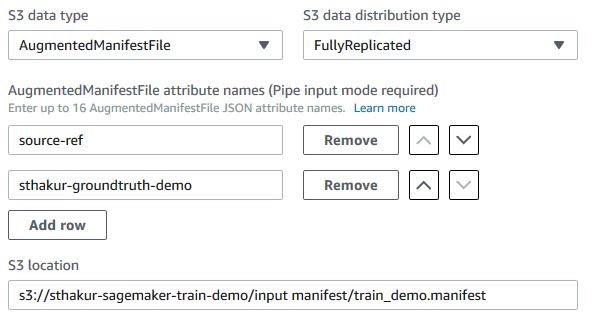
Choose the S3 data type as AugmentedManifestFile. Provide the Amazon S3 location of the manifest file from Step 1. Also provide the names of the JSON attributes that you want the Object Detection Algorithm to use from the augmented manifest file. Here we need only two attributes for training the model: source-ref and sthakur-groundtruth-demo as described in Step 1.

Since the JSON objects from the augmented manifest file are streamed in an ordered fashion using Amazon SageMaker Pipe mode, you need to carefully choose the sequence of attribute names that the algorithm should expect to find in the input data stream. Use the up and down arrow buttons next to each attribute name for choosing the sequence.

While we are showing here how to create an input data channel for sourcing training dataset, the Object Detection algorithm also requires an input data channel for validation dataset. One way to prepare the validation dataset would be to hold out a subset of your labeled images, and create another augmented manifest file for the validation set. You can then use the Amazon S3 URI of the new augmented manifest file as an input to your validation channel, and define the channel in exactly the same manner as described in this step.

Using the Amazon SageMaker Python SDK

We’ll use Amazon SageMaker Estimator to train the Object Detection Model.

od_model = sagemaker.estimator.Estimator(training_image,
                                         role, 
                                         train_instance_count=1, 
                                         train_instance_type='ml.p3.2xlarge',
                                         train_volume_size = 50,
                                         train_max_run = 360000,
                                         input_mode = 'Pipe',
                                         output_path=s3_output_location,
                                         sagemaker_session=sess)
…………………………..

train_data = sagemaker.session.s3_input(s3_train_data, distribution='FullyReplicated', content_type='image/jpeg', s3_data_type='AugmentedManifestFile', attribute_names=['source-ref', 'sthakur-groundtruth-demo'])

validation_data = sagemaker.session.s3_input(s3_validation_data, distribution='FullyReplicated', content_type='image/jpeg', s3_data_type='AugmentedManifestFile', attribute_names=['source-ref', 'sthakur-groundtruth-demo'])


…………………………………………..

data_channels = {'train': train_data, 'validation': validation_data}
od_model.fit(inputs=data_channels, logs=True)

Note that we’ve chosen the input_mode as Pipe, s3_data_type as AugmentedManifestFile, and specified the attribute_names sequence before training the model using SageMaker estimator’s fit routine.

Additional benefits of using augmented manifest format

Amazon SageMaker has always supported traditional manifest files for training models on datasets stored in Amazon S3. A manifest file simply provides a list of Amazon S3 key name prefixes for the data objects that need to be downloaded to Amazon SageMaker for training the model.

For example, this is a manifest file:

[
    {"prefix":"s3://foo/"},
  "relative/path/to/data-1",
  "relative/path/to/data-2",
  ...
]

Will match the following Amazon S3 URIs:

s3://foo/relative/path/to/data-1
s3://foo/relative/path/to/data-2

Using this traditional approach for specifying the input data channel for learning algorithms, such as visual recognition algorithms, requires you to specify two input data channels in Amazon SageMaker – one for the input data (images), and other for its labels. Using an augmented manifest, you can now put the data and its labels in one manifest file, thus reducing the need for two channels. It also eliminates any unnecessary complexity in algorithm code for matching data objects with labels across multiple channels.

For example, this manifest file can be easily expressed as an augmented manifest by restructuring the S3 URIs to JSON Lines format, and adding labels inline.

{"source-ref":"s3://foo/relative/path/to/data-1","label":"0"}
{"source-ref":"s3://foo/relative/path/to/data-2","label":"1"}
……….

Set attribute_names=['source-ref','label'] while training the model.

In addition, the augmented manifest file uses Amazon SageMaker Pipe mode, which means that your learning algorithm can benefit from the high throughput data streaming from Amazon S3 to your training instances in Amazon SageMaker. Here is a blog post that describes changes you can make to your learning algorithm to start consuming data using Pipe mode.

Get started with more examples and developer support

We’ve shown you examples of how to train models on Amazon SageMaker using labeled datasets in augmented manifest file format. You can also try out our sample notebook that provides the step-by-step AWS SDK experience. You can also see additional examples in our developer guide or post your questions on our developer forum.


About the Author

Sumit Thakur is a Senior Product Manager for AWS Machine Learning Platforms where he loves working on products that make it easy for customers to get started with machine learning on cloud. He is product manager for Amazon SageMaker and AWS Deep Learning AMI. In his spare time, he likes connecting with nature and watching sci-fi TV series.


Analyzing contact center calls—Part 1: Use Amazon Transcribe and Amazon Comprehend to analyze customer sentiment

Contact centers aiming to improve overall operational efficiency have an imperative to understand caller-agent dynamics. In part one of this two-part blog post series we’ll show you how you can use Amazon Transcribe and Amazon Comprehend to transform call recordings from audio to text and then run sentiment analysis on the transcripts. We will demonstrate how to use Amazon Transcribe to create text transcripts from an audio file. Afterwards, we’ll use Amazon Comprehend to analyze the call transcript, producing insights on keywords, topics, entities, and sentiment.

AWS services leveraged

Amazon Transcribe is an automatic speech recognition (ASR) service that makes it easy for developers to add speech-to-text capability to their applications. Using the Amazon Transcribe API, you can transcribe audio files stored in Amazon S3 into text transcripts.

Amazon Comprehend analyzes text and tells you what it finds, starting with the language, from Afrikaans to Yoruba, with 98 more in between. It can identify different types of entities (people, places, brands, products, and so forth), key phrases, sentiment (positive, negative, mixed, or neutral), and extract key phrases, all from text in English or Spanish. Finally, the Amazon Comprehend topic modeling service extracts topics from large sets of documents for analysis or topic-based grouping.

AWS Lambda lets you run code without provisioning or managing servers. You pay only for the compute time you consume – there is no charge when your code is not running.

AWS Step Functions makes it easy to coordinate the components of distributed applications and microservices using visual workflows.

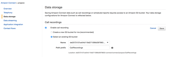
Amazon Connect is a self-service, cloud-based contact center service that makes it easy for any business to deliver better customer service at lower cost. Amazon connect produces Call Recordings between caller and Agent interactions.

Solution overview

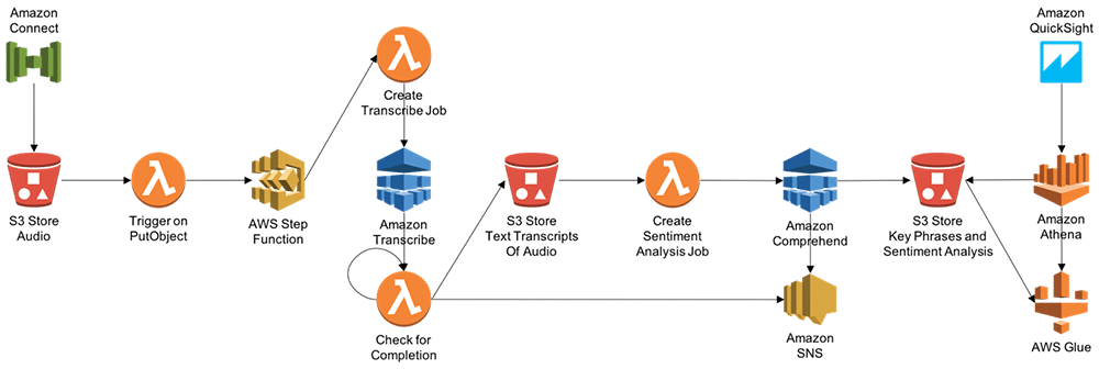
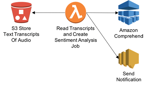
The architecture is broadly divided into these components, as the following diagram illustrates:

  1. Audio Transcript Storage → Amazon S3 bucket
  2. Orchestration component and business logic component → AWS Step Functions and AWS Lambda
  3. Transcribing component → Amazon Transcribe
  4. Sentiment analysis component → Amazon Comprehend
  5. Notification component → SNS Topic
  6. Amazon Comprehend → Entity, sentiment, key phrases, and language output into an Amazon S3 bucket
  7. AWS Glue maintains the database catalogue and database table structure. Amazon Athena queries data in Amazon S3 using the AWS Glue database catalogue.
  8. Amazon QuickSight analyzes call recording and performs sentiment, and performs a key phrases analysis of caller-agent interactions.

Transcribe call center audio, run sentiment analysis, and visualize analytics

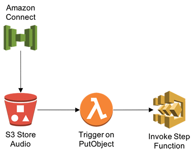
After uploading audio files to an Amazon S3 bucket, we’ll trigger a Lambda function to invoke Step Functions that will point the Amazon Transcribe service to the bucket destination to create transcription jobs. Accepted audio/visual formats include: WAV, FLAC, MP3, and MP4.

Step 1: Create the Lambda function and IAM policy

  1. Open the AWS Management Console and navigate to the Lambda console. Then choose Create a Lambda function.
  2. Choose Skip to skip the blueprint selection.
  3. For Runtime, choose Node JS 8.10.
  4. For Name, enter a function name.
  5. Enter a description that notes the source bucket and destination bucket used.
  6. For Code entry type, choose Edit code inline.
  7. Create environment variable – STEP_FUNCTIONS_ARN
  8. Paste the following into the code editor:
    'use strict';
    
    const aws = require('aws-sdk');
    
    var stepfunctions = new aws.StepFunctions();
    const s3 = new aws.S3({apiVersion: '2006-03-01'});
    
    exports.handler = (event, context, callback) => {
        const bucket = event.Records[0].s3.bucket.name;
        const key = decodeURIComponent(event.Records[0].s3.object.key.replace(/+/g, ' '));
        const params = {Bucket: bucket,Key: key};
    
        s3.getObject(params, (err, data) => {
            if (err) {
                console.log(err);
                const message = `Error getting object ${key} from bucket ${bucket}. Make sure they exist and your bucket is in the same region as this function.`;
                console.log(message);
                callback(message);
            } else {
                var job_name = key.replace("/", "-");
                var stepparams = {
                  "stateMachineArn": process.env.STEP_FUNCTIONS_ARN,
                   "input": "{"s3URL": "https://s3.amazonaws.com/" + bucket + "/" + key + "","JOB_NAME": ""+ job_name + ""}"
                };
                stepfunctions.startExecution(stepparams, function(err, data) {
                  if (err) console.log(err, err.stack); // an error occurred
                  else     console.log(data);           // successful response
                });
                callback(null, data.ContentType);
            }
        });
    };
    

Step 2: Create source Amazon S3 bucket

  1. Navigate to the Amazon S3 console and edit the source bucket configuration.
  2. Expand the Events section and provide a name for the new event.
  3. For Events, choose ObjectCreated (ALL).
  4. For Send to, choose Lambda Functions.
  5. For Lambda Function, select the Lambda function name you chose in Step 1.
  6. Choose Save

Step 3: Create Transcribe and Comprehend APIs using a Lambda function

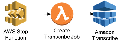
Trigger Transcribe job based on the input S3 audio transcript received. Two parameters are received – s3URL and JOB name.

  1. Navigate to the Lambda console, and then choose Create a Lambda function.
  2. Choose Skip to skip the blueprint selection.
  3. For Runtime, choose Node JS 8.10.
  4. For Name, enter a function name.
  5. Enter a description that notes Create Transcribe JOB based on the input received.
  6. For Code entry type, choose Edit code inline.
  7. Paste the following into the code editor:
    var AWS = require('aws-sdk');
    var transcribeservice = new AWS.TranscribeService();
    exports.handler = (event, context, callback) => {
        var params = {
          LanguageCode: 'en-US',
          Media: { /* required */
            MediaFileUri: event.s3URL + ""
          },
          MediaFormat: 'mp3',
          TranscriptionJobName: event.JOB_NAME
    
        };
        transcribeservice.startTranscriptionJob(params, function(err, data) {
          if (err) console.log(err, err.stack); // an error occurred
          else     {
          console.log(data);           // successful response
          event.wait_time = 60;
          event.JOB_NAME = data.TranscriptionJob.TranscriptionJobName;
          callback(null, event);
          }
        });
    
    };

Step 4: Get Transcribe Job Status

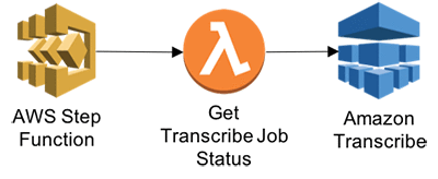
Get transcribe JOB status. This function will enable Step functions to wait for transcribe job to complete.

  1. In the Lambda console, choose Create a Lambda function.
  2. Choose Skip to skip the blueprint selection.
  3. For Runtime, choose Node JS 8.10.
  4. For Name, enter a function name.
  5. Enter a description that notes Transcribe JOB details.
  6. For Code entry type, choose Edit code inline.
  7. Paste the following into the code editor:
    var AWS = require('aws-sdk');
    var transcribeservice = new AWS.TranscribeService();
    
    exports.handler = (event, context, callback) => {
        var params = {
          TranscriptionJobName: event.JOB_NAME /* required */
        };
        transcribeservice.getTranscriptionJob(params, function(err, data) {
          if (err) console.log(err, err.stack); // an error occurred
          else     console.log(data);           // successful response
          event.STATUS = data.TranscriptionJob.TranscriptionJobStatus;
          event.Transcript =data.TranscriptionJob.Transcript;
          callback(null,event);
        });
    };

Step 5: Get transcribe job details

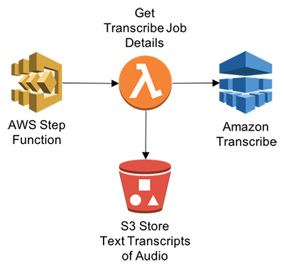
This function will enable Step Functions to get transcribe JOB details once completed.

  1. In the Lambda console, choose Create a Lambda function.
  2. Choose Skip to skip the blueprint selection.
  3. For Runtime, choose Node JS 8.10.
  4. For Name, enter a function name.
  5. Enter a description that notes get information about the transcribe job.
  6. For Code entry type, choose Edit code inline.
  7. Paste the following into the code editor:
    var AWS = require('aws-sdk');
    var transcribeservice = new AWS.TranscribeService();
    
    exports.handler = (event, context, callback) => {
    
        var params = {
          TranscriptionJobName: event.JOB_NAME /* required */
        };
        transcribeservice.getTranscriptionJob(params, function(err, data) {
          if (err) console.log(err, err.stack); // an error occurred
          else     console.log(data);           // successful response
          event.STATUS = data.TranscriptionJob.TranscriptionJobStatus;
          event.TranscriptFileUri =data.TranscriptionJob.Transcript.TranscriptFileUri;
          callback(null,event);
        });
    };

Step 6: Call Amazon Comprehend to analyze transcription text

In this step, you’ll get transcribed audio text and perform contextual analysis. This function will enable Step Functions to call Amazon Comprehend to perform sentiment analysis.

  1. In the Lambda console, choose Create a Lambda function.
  2. Choose Skip to skip the blueprint selection.
  3. For Runtime, choose Node JS 8.10.
  4. For Name, enter a function name.
  5. Enter a description that notes get information about the transcribe job.
  6. For Code entry type, choose Edit code inline.
  7. Paste the following into the code editor:
    var https = require('https');
    let AWS = require('aws-sdk');
    var comprehend = new AWS.Comprehend({apiVersion: '2017-11-27'});
    exports.handler = function(event, context, callback) {
        var request_url = event.request_url;
        https.get(request_url, (res) => {
          var chunks = [];
    	  res.on("data", function (chunk) {
            chunks.push(chunk);
          });
          res.on("end", function () {
            var body = Buffer.concat(chunks);
            var results = JSON.parse(body);
            console.log( body.toString());
            var transcript = results.results.transcripts[0].transcript;
            console.log(transcript)
            var params = {
              LanguageCode: "en",
              Text: transcript + ""
            };
            comprehend.detectSentiment(params, function(err, data) {
              if (err) console.log(err, err.stack); // an error occurred
              else     console.log(data);           // successful response
              callback(null, data);
            });
            callback(null, transcript);      });
    
    	}).on('error', (e) => {
    	  console.error(e);
    	});
    };

Step 7: Invoke Step Functions

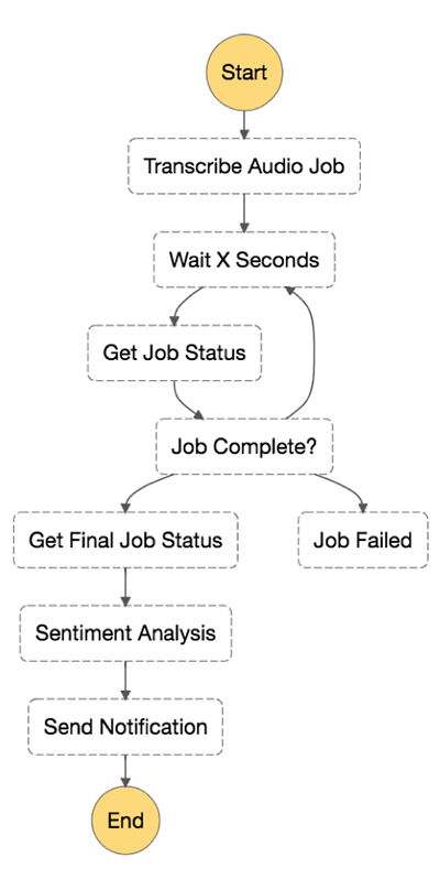
In this step you will leverage AWS Steps Functions orchestrate the Lambda functions created earlier and notify the end customer about the contextual analysis.

  1. In the Step Functions console, choose Create a state machine.
  2. Choose Author from scratch
  3. For Name,  Enter your State Machine Name For example : TranscribeJob.
  4. Paste the following code in State machine definition
  5. Update the ARN values of lambda functions created in earlier steps in the State machine definition code
  6. Click Next
  7. Choose existing role which has permissions to invoke lambda functions, send SNS (Create the custom role if the role doesn’t exists)
  8. Click Create state machine


{
	"Comment": "A state machine that submits a Job to AWS Batch and monitors the Job until it completes.",
	"StartAt": "Transcribe Audio Job",
	"States": {
		"Transcribe Audio Job": {
			"Type": "Task",
			"Resource": "<<Start Transcribe job for Audio to Text ARN>>",
			"ResultPath": "$",
			"Next": "Wait X Seconds",
			"Retry": [{
				"ErrorEquals": ["States.ALL"],
				"IntervalSeconds": 1,
				"MaxAttempts": 3,
				"BackoffRate": 2
			}]
		},
		"Wait X Seconds": {
			"Type": "Wait",
			"SecondsPath": "$.wait_time",
			"Next": "Get Job Status"
		},
		"Get Job Status": {
			"Type": "Task",
			"Resource": "<<Get Transcribe job status ARN>>",
			"Next": "Job Complete?",
			"InputPath": "$",
			"ResultPath": "$",
			"Retry": [{
				"ErrorEquals": ["States.ALL"],
				"IntervalSeconds": 1,
				"MaxAttempts": 3,
				"BackoffRate": 2
			}]
		},
		"Job Complete?": {
			"Type": "Choice",
			"Choices": [{
				"Variable": "$.STATUS",
				"StringEquals": "IN_PROGRESS",
				"Next": "Wait X Seconds"
			}, {
				"Variable": "$.STATUS",
				"StringEquals": "COMPLETED",
				"Next": "Get Final Job Status"
			}, {
				"Variable": "$.STATUS",
				"StringEquals": "FAILED",
				"Next": "Job Failed"
			}],
			"Default": "Wait X Seconds"
		},
		"Job Failed": {
			"Type": "Fail",
			"Cause": "AWS Batch Job Failed",
			"Error": "DescribeJob returned FAILED"
		},
		"Get Final Job Status": {
			"Type": "Task",
			"Resource": "<<Get Transcribe job details ARN>>",
			"InputPath": "$",
			"Next": "Send contextual analysis"
			"Retry": [{
				"ErrorEquals": ["States.ALL"],
				"IntervalSeconds": 1,
				"MaxAttempts": 3,
				"BackoffRate": 2
			}]
		},
		
		"Send contextual analysis": {
			"Type": "Task",
			"Resource": "<<Send Contextual Analysis ARN>>",
			"InputPath": "$",
			"End": true,
			"Retry": [{
				"ErrorEquals": ["States.ALL"],
				"IntervalSeconds": 1,
				"MaxAttempts": 3,
				"BackoffRate": 2
			}]
		}
	}
}

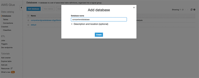
Step 8: Create an AWS Glue database for visualization

Navigate to the AWS Glue console and create a database to store sentiment analysis entities.

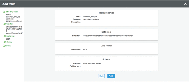
Add the AWS Glue table to the database you just created.


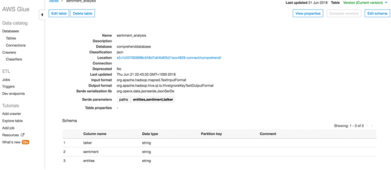
A created table in database looks like this:

Step 9: Visualization using Amazon QuickSight

To visualize Amazon Comprehend output using Amazon QuickSight, do the following:

  1. Connect Amazon QuickSight to Amazon Athena.
    1. https://docs.aws.amazon.com/quicksight/latest/user/create-a-data-set-athena.html
    2. https://docs.aws.amazon.com/quicksight/latest/user/managing-permissions.html
    3. https://aws.amazon.com/blogs/big-data/derive-insights-from-iot-in-minutes-using-aws-iot-amazon-kinesis-firehose-amazon-athena-and-amazon-quicksight/
  2. Grant Amazon QuickSight access to Athena and the associated S3 buckets in the account. For information on how to do this, see Managing Amazon QuickSight Permissions to AWS Resources in the Amazon QuickSight User Guide.
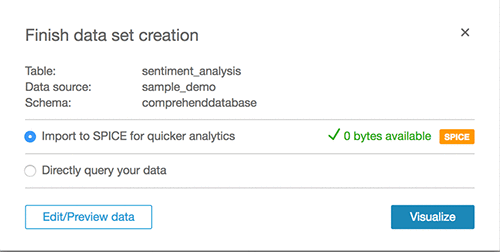
  3. Create a new data set for visualising sentiment analysis in Amazon QuickSight based on the Athena table that was created during deployment.

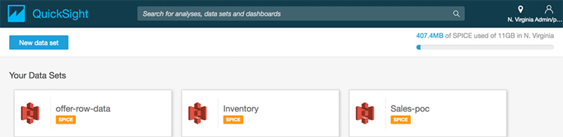
After setting up permissions, create a new analysis in Amazon QuickSight by choosing New analysis.

Add a new data set.

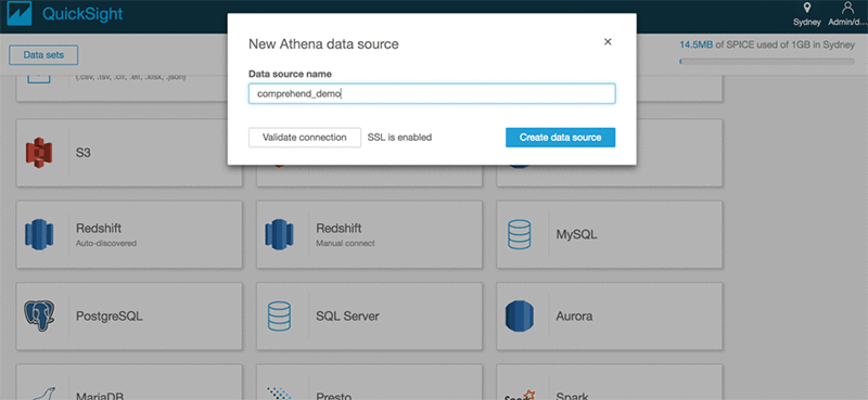
Choose Athena as the source and give the data source a name, such as comprehend_demo.

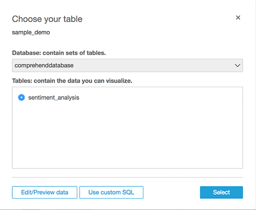
Click Select to choose the database and table.

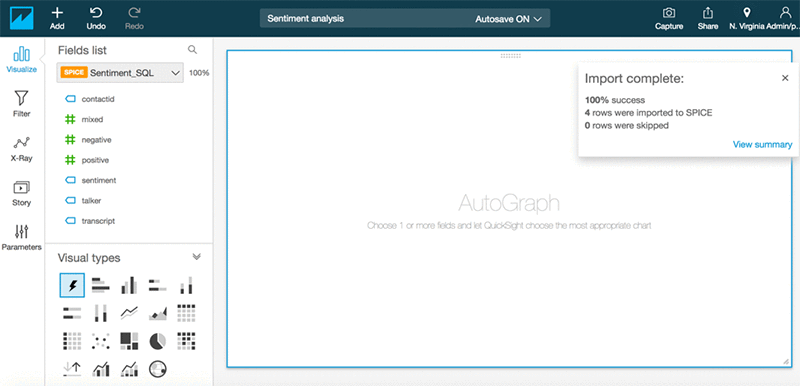
Click Visualize.

Create custom visualizations.

Conclusion

Enterprises can reap significant benefits by realizing the hidden value in the massive amounts of caller-agent audio recordings from their contact centers. By deriving meaningful insights, enterprises can enhance both efficiency and performance of call centers and improve their overall service quality to end customers. So far, we’ve used Amazon Transcribe to transform audio data into text transcripts and then used Amazon Comprehend to run text analysis. Along the way, we’ve also used AWS Lambda and AWS Step Functions to string together the solution. And finally, AWS Glue, Amazon Athena, and AWS QuickSight to visualize the analysis. The AWS CloudFormation templates used to build and deploy this process are available on part 2 of the next post.

In Part 2 of this blog post series we’ll show you how to automate, deploy, and visualize analytics using Amazon Transcribe, Amazon Comprehend, AWS CloudFormation, and Amazon QuickSight.

About the Authors

Deenadayaalan Thirugnanasambandam is a Senior Cloud Architect in the Professional Services team in Australia.


Piyush Patel is a big data consultant with AWS.


Paul Zhao is a Sr. Product Manager at AWS Machine Learning. He manages the Amazon Transcribe service. Outside of work, Paul is a motorcycle enthusiast and avid woodworker.


Revanth Anireddy is a professional services consultant with AWS.


Loc Trinh is a Solutions Architect for AWS Database and Analytics services. In his spare time, he captures data from his eating and fitness habits and uses analytical modeling to determine why he is still out of shape.


Scalable multi-node training with TensorFlow

We’ve heard from customers that scaling TensorFlow training jobs to multiple nodes and GPUs successfully is hard. TensorFlow has distributed training built-in, but it can be difficult to use. Recently, we made optimizations to TensorFlow and Horovod to help AWS customers scale TensorFlow training jobs to multiple nodes and GPUs. With these improvements, any AWS customer can use an AWS Deep Learning AMI to train ResNet-50 on ImageNet in just under 15 minutes.

To achieve this, 32 Amazon EC2 instances, each with 8 GPUs, a total 256 GPUs, were harnessed with TensorFlow. All of the required software and tools for this solution ship with the latest Deep Learning AMIs (DLAMIs), so you can try it out yourself. You can train faster, implement your models faster, and get results faster than ever before. This blog post describes our results and shows you how to try out this easier and faster way to run distributed training with TensorFlow.

Figure A. ResNet-50 ImageNet model training with the latest optimized TensorFlow with Horovod on a Deep Learning AMI takes 15 minutes on 256 GPUs.

Training a large model takes time, and the larger and more complex the model is, the longer the training is going to take. If your business requirement is to generate updated models on a regular basis, any training that takes too long means missed opportunities. A typical response is to throw more processing power at the problem, but for deep learning, the communications overhead during training has made this approach infeasible or profoundly expensive. This communications overhead results in a loss of efficiency, significantly reducing your throughput and increasing your time to train. It can also be complex to set up the required infrastructure and reach required levels of accuracy. TensorFlow supports distributed training natively, but in our experiments, we obtained better results (in both speed and accuracy) when we incorporated Horovod.

Horovod is a popular choice for distributed training. Take, for example, the recent use of Horovod with 27,000 GPUs to analyze climate change. Orchestrating this number of GPUs would be impossible without proper tooling. With Horovod, using software optimizations and Amazon EC2 p3 instances, we were able to limit the efficiency loss to 15 percent, resulting in a time-to-train under 15 minutes.
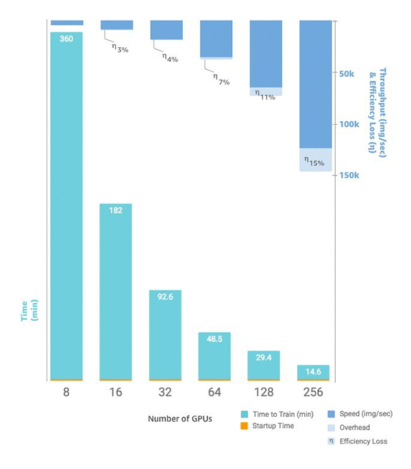
Figure B. Time to train vs number of GPUs vs images per second, communication overhead, and efficiency. Startup time is a consistent 1.5 minutes regardless of cluster size.

All of the tools you need to try this out are shipped on the latest DLAMI. This includes example scripts for training ResNet-50 with ImageNet. If you’re ready to roll up your sleeves now and try it out, continue reading. The rest of this blog post shows you how you can use EC2 p3 instances, TensorFlow, and Horovod to train ResNet-50 on ImageNet in under 15 minutes.

How to train ResNet/ImageNet in under 15 minutes with TensorFlow

I first tried out Horovod with TensorFlow on the Deep Learning AMI (DLAMI). I was asked to write a tutorial on using Horovod to train ImageNet on an eight-GPU EC2 instance. I wondered what on earth was Uber thinking when they named their distributed training framework “Horovod”, and I wondered how much time was this going to take? Training ImageNet takes forever, and Horovod sounds like some villain from the Harry Potter universe. It’s not. It was created by Alexander Sergeev at Uber. He named it after Russian & eastern European folk dance where a large group of dancers perform synchronized moves in a circle. It turned out to be a fun way to learn how to dance with Horovod using up to 8 GPUs in one DLAMI.

That was a couple of months ago, and now I’m going to show you what the the TensorFlow team here at Amazon AI has been up to. They’ve been fine-tuning Horovod with TensorFlow, and the implementation on the DLAMI is much faster. More importantly, you can run upwards of 256 GPUs in one training run to train ResNet-50 on ImageNet in under 15 minutes!

The first time I ran Horovod on a DLAMI was on a p3.16xlarge EC2 instance. This beast of an instance has eight Tesla V100 GPUs. Horovod uses all of the instance’s GPUs  to turn a training time that could take more than a day to a training time that could be finished in a few hours. I used the latest DLAMI so I wouldn’t have to install and configure CUDA, TensorFlow, or Horovod. I could activate the environment with one command, and then execute the training script with another one liner.

Setup was easy. Training was relatively fast – only slightly sub-linear scaling from one to eight GPUs. It finished in eight hours and the accuracy was acceptable: 75.4% for top-1 and 92.6% for top-5. Based on this result, I wrote the Tensorflow-Horovod tutorial for the DLAMI .

Next, I asked myself how fast I can train ResNet-50 on several p3 instances. I knew that scaling efficiency will never be 100% and that, in total, people will end up paying more. However, if your team was waiting for a model to train for a day, they would think training in 15 minutes was worth the savings on developers’ productivity. This is especially true because the efficiency loss of the faster training, as our experiments demonstrate, is minimal.

We recently benchmarked running 256 GPUs with great accuracy and an even faster completion time. Don’t you want to try that out yourself? Does your dance card even have 256 slots? Keep reading and I’ll walk you through how we can make this happen.

With the latest updates to the DLAMI and its TensorFlow-Horovod environment you could train ResNet-50 on all of ImageNet for about a 20% cost reduction compared to its release. In this blog post we’ll demonstrate how fast things can go and scale, and save your wallet for future dances with Horovod. Are you ready?

The original TensorFlow-Horovod tutorial shows you a single node implementation. You spin up one instance and use all of its GPUs. This time I’ll show you how you can spin up several nodes, link them up with a Horovod configuration, and then run the training. We’ll run some benchmarks, so you can estimate your time for completion and see what your efficiency loss is for each new node. With this info you can estimate your costs, and then apply this pattern to other models that you want to train.

Part 1: Spin up a bunch of DLAMIs

Now is a good time to plan out your moves with a quick questionnaire:

  1. Do you need to get a copy of ImageNet?
    1. If yes:
      1. Spin up one DLAMI for now. Downloading and prepping the dataset can take several hours, and you don’t want several instances sitting around, racking up your bill while you wait. You can add more DLAMIs later. If you want to be clever, you can run the download and prep steps faster with a big DLAMI CPU instance, then transfer it to your DLAMI GPU instances for training when it is ready. You could also divide up the dataset and prep the dataset across multiple machines.
    2. If no: go to 2.
  2. Do you have an ImageNet dataset already downloaded to your AWS environment – on Amazon S3, a shared volume, or on an instance?
    1. If yes:
      1. Later in this blog I’ll give you some bash functions that can help you distribute the dataset to each node.
    2. If no:
      1. Only spin up one instance for now. Get it ready there, then spin up the rest and distribute the dataset using one of the functions I just mentioned.
  3. Is your ImageNet dataset already preprocessed for training with TensorFlow?
    1. If yes:
      1. You’re going to be able to do everything in this blog post pretty quickly, even train ImageNet entirely in about an hour-and-a-half with just four instances.
    2. If no:
      1. Follow these detailed instructions in DLAMI’s docs on how to prepare the ImageNet dataset.

Now let’s spin up one or more DLAMIs. There are several ways you can do this, but I’m going to use the Amazon EC2 console. If you already know how to use AWS Cloud Formation templates or the AWS CLI, you can use those tools as well. The goal here is to launch some number of identical DLAMIs that each have more than one GPU. For this next step, I’m going to launch four p3.16xlarge DLAMIs all in the same Region and security zone (VPC). This step is important. You can’t just link up random instances you have that are launched in different Regions or security zones without impacting performance.

On the EC2 console you can search for an AMI by name. Search for “deep learning” and you will find Deep Learning AMI (Ubuntu). Choose the Select button.
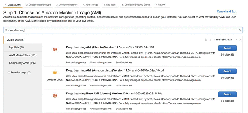
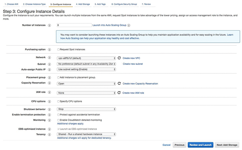
After you select the Deep Learning AMI (Ubuntu) you can choose the instance type. Since we want to use the faster instance to achieve the fastest training, choose the p3dn.24xl instance type. If this is not available yet in your Region, choose the p3.16xlarge instead. The more GPUs you have on the same system, the faster your training will be. Now choose Next: Configure Instance Details. You have the option of launching multiple identical instances. Choose up to 32 instances to achieve 256 GPU training. For the purposes of this example, however, I’ll use 4 instances, with a total of 32 GPUs.
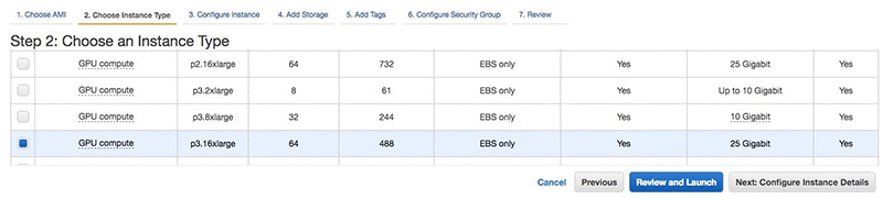
Next, choose your instance details.  You should choose an instance with at least 200 GB of fast storage. I’m choosing a Provisioned IOPS SSD with 10,000 IOPS to get the best performance.
You can just skip through the tags screen and continue to Configure Security Group.

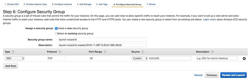
On the security group settings page, you can create a new group, or use an existing one. Next, review your choices, make corrections as needed, and then choose Review and Launch.
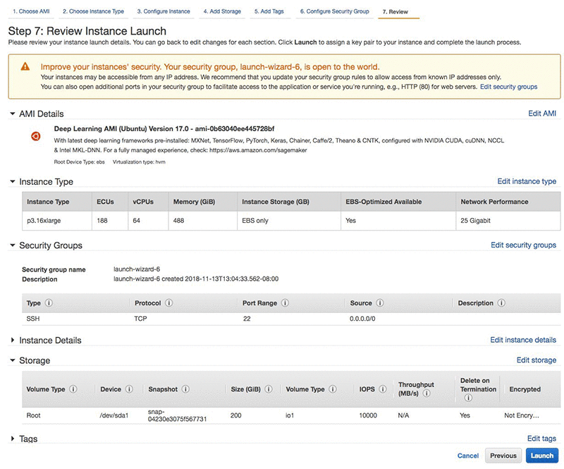
Your screen should look much like the following screenshot. Important things to note are in the storage section: size, volume type, and IOPS.  Choose Launch.
After choosing Launch, you’ll select a key pair. Use existing keys or create new ones. Make note of where you put your keys and what you named them because you will need this information later.

If you get a green box, choose View Instances to review the list of the freshly launch DLAMIs.

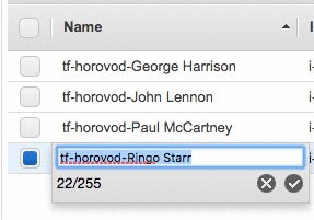
It takes a couple of minutes to launch the instances, so now is a good time to name them.

Select one of your DLAMIs. Rename it in the console so you don’t forget which one is which. If you have 8 nodes, you could call them Snow White and the Seven Dwarves (Doc, Dopey, Bashful, Grumpy, Sneezy, Sleepy, and Happy). I only launched four, so I called them John Lennon, Paul McCartney, George Harrison, and Ringo Starr. I chose John Lennon to be the leader. Some people like to call the leader the master, but I prefer “leader.” There’s a leader and members.
Part 2: Prep the dataset

Step 1. Download a copy of ImageNet to each new cluster of DLAMIs. 

For the fastest performance you will want each instance in your cluster to have a local copy of the dataset. The raw dataset needs to be preprocessed by a TensorFlow utility before you train with it. Otherwise, training will take longer, and you won’t see the accuracy levels that are reported in most benchmarks. If you don’t have ImageNet handy, you’ll need to download it. Even if you do have a copy, you will need this data to be inside your cluster’s Region and security zone, and it will need that previously mentioned preprocessing. So, if you have a preprocessed copy ready on Amazon S3 or elsewhere, great, copy it to your leader, then you can skip ahead to Part 3.

Download ImageNet to one of your instances now, or if you already have it somewhere, copy it to an instance now, and then read ahead. This way you’ll know what is coming, and in Part 3 you can try out distributed training with a synthetic dataset while you wait.

Step 2. Prep the ImageNet files for training.

You need to run a preparation step prior to training. This preprocesses all of the images, so that they’re consistent and optimized for training speed. Without running this step you can’t hope to achieve comparable speed or accuracy. Your costs will certainly be higher. Note that after you run this step once, you don’t have to do it again for subsequent training runs. You might want to keep this volume around and connect it to future DLAMIs and tests or benchmarking runs.

Follow these detailed instructions in DLAMI’s docs on how to prepare the ImageNet dataset.

I must admit that I already had my preprocessed copy of ImageNet sitting around, so that’s why I said the setup and training was so easy. Now that you’ve done the preprocessing, you’ll want to keep yours too. You can stop any one of your instances without terminating it, then bring the instance back along with the data sometime in the future! You could also save the preprocessed dataset to S3 to archive it for later use.

Part 3: training with synthetic data

While you wait for ImageNet to download, you can try the setup with synthetic data. This will assure that your members can talk to each other, TensorFlow with Horovod is working in this multi-node mode, and that eventually you can switch to training with the ImageNet dataset.

Before you move on to the next step, review the overall settings, making sure each node is running, is the same instance type and is in the same Availability Zone.

In the console, choose the leader, choose the Actions button, and then choose Connect. The next page provides instructions for connecting. If you created a new key, you will need to adjust its security settings with chmod 400 key.pem. These instructions are in the Connect prompt. However, one important variation in how you connect with ssh is that you want your leader to be able to access your members. You do this by adding your key and customizing your ssh login to be slightly different than what is suggested by the Connect prompt. Run the following commands from your local terminal and the directory where you downloaded your key. Be sure to swap out “key.pem” with the filename of the key and “PUBLIC_IP_ADDRESS_OF_THE_LEADER” before running it.

ssh-add -K key.pem
ssh -A ubuntu@PUBLIC_IP_ADDRESS_OF_THE_LEADER

Once connected, activate the tensorflow_p36 environment.
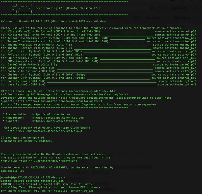
In this example, I’m launching John Lennon now. After I have logged in, I’ll start the TensorFlow environment. You will likely see TensorFlow being optimized for the instance type, so this first activation may take a moment.

source activate tensorflow_p36

After activating the environment we must let Horovod know about the rest of the band. This is achieved by adding each member’s info to a hosts file. Change directories to where the training scripts reside.

cd ~/examples/horovod/tensorflow

Use vim to edit a file in the leader’s home directory.

vim hosts

Select one of the members in the EC2 console, and the description page opens. Find the Private IPs field and copy the IP address and paste it in a text file. Copy each member’s private IP address on a new line. Then, next to each IP address add a space and then the text slots=8. This represents how many GPUs each instance has. The p3.16xlarge instances have 8 GPUs, so if you chose a different instance type, you would provide the actual number of GPUs for each instance. For the leader you can use localhost. It should look similar to the following:

172.100.1.200 slots=8
172.200.8.99 slots=8
172.48.3.124 slots=8
localhost slots=8

Save the file and exit back to the leader’s terminal.

Now your leader knows how to reach each member. This is all going to happen on the private network interfaces. Next, use a short bash function to help send commands to each member. Run this command in your leader’s terminal session:

function runclust(){ while read -u 10 host; do host=${host%% slots*}; ssh -o "StrictHostKeyChecking no" $host ""$2""; done 10<$1; };

First tell the other members to not do “StrickHostKeyChecking” as this may cause training to hang.

runclust hosts "echo "StrictHostKeyChecking no" >> ~/.ssh/config"

Now it is time to try out the training with synthetic data. The script deep-learning-models/models/resnet/tensorflow/dlami_scripts/train_synthetic.sh will default to 8 GPUs, but you can provide it the number of GPUs you want to run. Run the script, passing 4 as a parameter for the 4 GPUs we’re using for this run.

$ ./train_synthetic.sh 4

After some warning messages you will see the following output that verifies Horovod is using 4 GPUs.

PY3.6.5 |Anaconda custom (64-bit)| (default, Apr 29 2018, 16:14:56) 
[GCC 7.2.0]TF1.11.0
Horovod size: 4

Then after some other warnings you see the start of a table and some data points. You break out of the training if you don’t want to watch for 1,000 batches. Here I stop it at 400 since I can see that the training is averaging about 3,000 images per second.

   Step Epoch  Speed  Loss   FinLoss LR
     0   0.0   105.6  6.794  7.708 6.40000
     1   0.0   311.7  0.000  4.315 6.38721
   100   0.1  3010.2  0.000 34.446 5.18400
   200   0.2  3013.6  0.000 13.077 4.09600
   300   0.2  3012.8  0.000  6.196 3.13600
   400   0.3  3012.5  0.000  3.551 2.30401

Let’s try 8 GPUs.

./train_synthetic.sh 8

I stopped at 200 this time once I saw that the speed was a little less than double: 5,874 vs 3,012.

   Step Epoch  Speed  Loss   FinLoss LR
    0    0.0   200.5  6.804   7.718 6.40000
    1    0.0   564.2  0.000   6.878 6.38721
  100    0.2  5871.7  0.000  60.158 5.18400
  200    0.3  5874.3  0.000  22.838 4.09600

Now you’re ready to test multi-node training. Try out the full 32 GPUs.

./train_synthetic.sh 32

Your output will be similar. You will see the Horovod size at 32, and you will see roughly 4 times the speed. With this experimentation completed, you will have tested your leader and its ability to communicate with the members. If you run into any issues, check the troubleshooting section in the Horovod tutorials docs.

Part 4: Train ResNet-50 on ImageNet

After you’re satisfied watching the synthetic data training step and you’ve prepared the ImageNet dataset, you’re ready to copy the prepared dataset to all of the members.

If you still only have the dataset on your leader, use this copyclust function to copy data over to other members. Run this command in your leader’s terminal session:

function copyclust(){ while read -u 10 host; do host=${host%% slots*}; rsync -azv "$2" $host:"$3"; done 10<$1; };

Now you can use copyclust to copy the dataset folder. The first param is the hosts file, the second is the dataset folder on your leader, and the third is the target directory on each member:

copyclust hosts ~/imagenet_data ~/imagenet_data

Or, if you have the files sitting in an Amazon S3 bucket, use the runclust function to download the files to each member directly.

runclust hosts "tmux new-session -d "export AWS_ACCESS_KEY_ID=YOUR_ACCESS_KEY && export AWS_SECRET_ACCESS_KEY=YOUR_SECRET && aws s3 sync s3://your-imagenet-bucket ~/imagenet_data/ && aws s3 sync s3://your-imagenet-validation-bucket ~/imagenet_data/""

There’s something to be said here about using tmux or screen or some tools to let you disconnect and resume sessions. Using tools that let you manage multiple nodes at once is a great timesaver. But, I’m going to gloss over this part because it goes beyond the scope of this blog. You have many options: wait around for each step and manage each instance separately or use some power tools.

After the copying is completed, you’re ready to start training. Run the script, passing 32 as a parameter for the 32 GPUs we’re using for this run. Use tmux or a similar tool if you’re concerned about disconnecting and terminating your session, thereby aborting the training run.

./train.sh 32

The following output is what you see when running the training on ImageNet with 32 GPUs. 32 GPUs will take 90-110 minutes.

   Step Epoch  Speed  Loss   FinLoss LR
     0   0.0   440.6  6.935  7.850 0.00100
     1   0.0  2215.4  6.923  7.837 0.00305
    50   0.3 19347.5  6.515  7.425 0.10353
   100   0.6 18631.7  6.275  7.173 0.20606
   150   1.0 19742.0  6.043  6.922 0.30860
   200   1.3 19790.7  5.730  6.586 0.41113
   250   1.6 20309.4  5.631  6.458 0.51366
   300   1.9 19943.9  5.233  6.027 0.61619
   350   2.2 19329.8  5.101  5.864 0.71872
   400   2.6 19605.4  4.787  5.519 0.82126
   450   2.9 20025.5  5.020  5.725 0.92379
   500   3.2 19526.8  4.702  5.383 1.02632
   550   3.5 18102.1  4.632  5.294 1.12885
   600   3.8 19450.3  4.377  5.023 1.23138
   650   4.2 19845.1  3.738  4.372 1.33392
   700   4.5 18838.6  3.862  4.488 1.43645
   750   4.8 19572.7  3.435  4.059 1.53898
   800   5.1 20697.7  3.388  4.015 1.64151
   850   5.4 19651.1  3.141  3.774 1.74405
   900   5.8 20012.3  3.231  3.878 1.84658
   950   6.1 19261.0  3.039  3.699 1.94911
  1000   6.4 18248.2  2.969  3.645 2.05164
  1050   6.7 18730.4  2.731  3.429 2.15417
  ...
   13750  87.9 19398.8  0.676  1.082 0.00217
 13800  88.2 19827.5  0.662  1.067 0.00156
 13850  88.6 19986.7  0.591  0.997 0.00104
 13900  88.9 19595.1  0.598  1.003 0.00064
 13950  89.2 19721.8  0.633  1.039 0.00033
 14000  89.5 19567.8  0.567  0.973 0.00012
 14050  89.8 20902.4  0.803  1.209 0.00002
Finished in 6004.354426383972

This run completed! It follows up with an evaluation run. It will run on the leader as it will run quickly enough without having to distribute the job to the other members. The following is the output of the evaluation run.

Horovod size: 32
Evaluating
Validation dataset size: 50000
 step  epoch  top1    top5     loss   checkpoint_time(UTC)
14075   90.0  75.716   92.91    0.97  2018-11-14 08:38:28

If you’re curious what this output looks like with 256 GPUs, you can check it out in the following output block.

  Step Epoch  Speed    Loss   FinLoss LR
  1550  79.3 142660.9  1.002  1.470 0.04059
  1600  81.8 143302.2  0.981  1.439 0.02190
  1650  84.4 144808.2  0.740  1.192 0.00987
  1700  87.0 144790.6  0.909  1.359 0.00313
  1750  89.5 143499.8  0.844  1.293 0.00026
Finished in 860.5105031204224

Finished evaluation
1759   90.0  75.086   92.47    0.99  2018-11-20 07:18:18

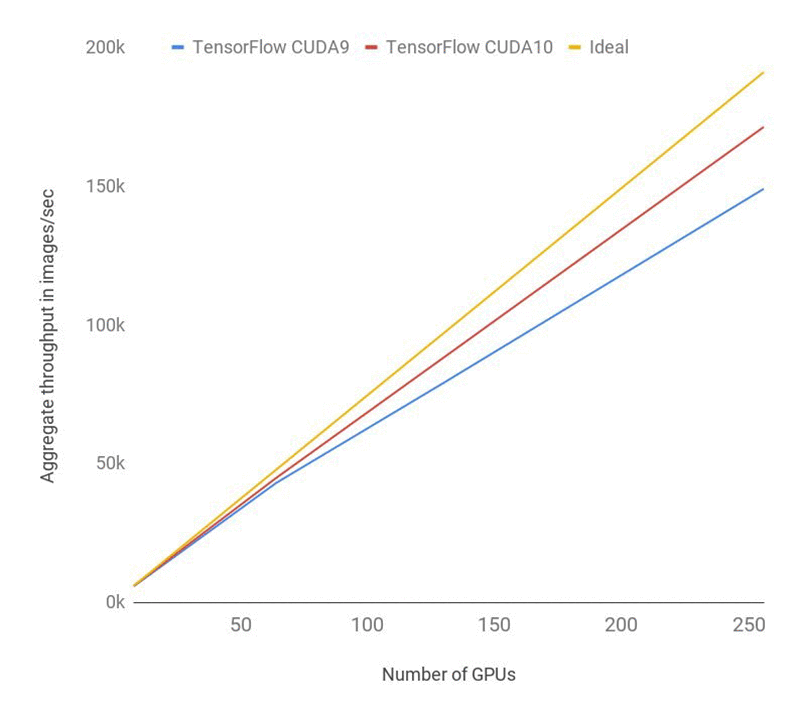
You can see that the speed in images/sec is over 140k. The following chart shows the latest benchmarks with CUDA10 using 256 GPUs which reaches speeds of 171k! This improves efficiency to 90%. Look for this to ship on the DLAMI after TensorFlow releases an official binary for CUDA 10.  The following chart shows the Performance of ResNet-50 training using CUDA 10. Overhead is reduced compared to CUDA 9.
Conclusion

Now that you’ve tried four nodes, do you want to try more? How about 16 or 32 nodes? Or how about 2? You can scale up or down and see how that impacts performance. Compare epoch training times and estimate your overall cost for completion.

Note: if you use the “more like this” feature in the Amazon EC2 console, be prepared to adjust all of the settings, most notably the storage. “More like this” doesn’t include storage, so make sure you update that to have at least 200 GB.

You might want to also try a different dataset and see how fast you can train it using the latest instance types and optimized TensorFlow environments on the DLAMI.

Stay tuned for our next blog where we apply the latest improvements in scalable training on a cluster of DLAMIs.


Appendix

Troubleshooting

The following command might help you get past errors that come up when you experiment with Horovod.

  • If the training crashes, mpirun may fail to clean up all the Python processes on each machine. In that case, before you start the next job kill the Python processes on all machines as follows:
    • runclust hosts “pkill -9 python”
  • If the process finishes abruptly without error, try deleting your log folder.
  • If other unexplained issues pop up, check your disk space. If you’re out of space, try removing the logs folder since that is full of checkpoints and data. You can also increase the size of the volumes for each member.
  • As a last resort you can also try rebooting.
# kill python
runclust hosts "pkill -9 python"
# delete log folder
runclust hosts "rm -rf ~/imagenet_resnet/"
# check disk space
runclust hosts "df /"
# reboot
runclust hosts "sudo reboot"

About the Author

Aaron Markham is a programmer writer for MXNet and AWS Deep Learning AMI. He has a degree in winemaking and a passion for new technology which he shares by writing and teaching. Aside from talking about deep learning tech, he teaches computer skills to the homeless in Santa Cruz and web programming to prisoners at San Quentin. When not working or teaching, you can find him on the slopes snowboarding or hiking.


Soft Actor Critic—Deep Reinforcement Learning with Real-World Robots

We are announcing the release of our state-of-the-art off-policy model-free
reinforcement learning algorithm, soft actor-critic (SAC). This algorithm has
been developed jointly at UC Berkeley and Google, and we have been using
it internally for our robotics experiment. Soft actor-critic is, to our
knowledge, one of the most efficient model-free algorithms available today,
making it especially well-suited for real-world robotic learning. In this post,
we will benchmark SAC against state-of-the-art model-free RL algorithms and
showcase a spectrum of real-world robot examples, ranging from manipulation to
locomotion. We also release our implementation of SAC, which is particularly
designed for real-world robotic systems.

Continue reading

Amazon SageMaker Automatic Model Tuning now supports early stopping of training jobs

In June 2018, we launched Amazon SageMaker Automatic Model Tuning, a feature that automatically finds well-performing hyperparameters to train a machine learning model with. Unlike model parameters learned during training, hyperparameters are set before the learning process begins. A typical example of the use of hyperparameters is the learning rate of stochastic gradient procedures. Using default hyperparameters doesn’t always yield the best model performance, and finding well-performing hyperparameters can be a non-trivial and time-consuming task. Using Automatic Model Tuning, Amazon SageMaker will automatically find well-performing hyperparameters and train your model to maximize your objective metric.

The number of possible hyperparameter configurations is exponential in the number of hyperparameters that are being explored. A naive exploration of this search space would require a large number of training jobs and would result in high cost. To overcome this, Amazon SageMaker uses Bayesian optimization, a strategy that efficiently models the performance of different hyperparameters based on a small number of training jobs. This algorithm will, however, at times explore hyperparameter configurations which, by the end of the training, turn out to be significantly worse than previous configurations.

Today, we are adding the early stopping feature to Automatic Model Tuning. By enabling early stopping when you launch a tuning job, Amazon SageMaker tracks objective metrics per training iteration (‘epoch’) for each candidate model. Amazon SageMaker then assesses how likely each candidate is to outperform the previous best model evaluated thus far in your tuning job. With early stopping those models that are unlikely to bring value are terminated before completing all iterations, saving time and reducing cost by up to 28% (depending on your algorithm and dataset). For example, in this blog post we show how to use early stopping with an image classification algorithm using Amazon SageMaker, reducing time and cost by 23%.

You can use early stopping with supported built-in Amazon SageMaker algorithms and with your own algorithms, provided that they emit objective metrics per epoch.

Tuning an image classification model that uses early stopping

To demonstrate how you can leverage early stopping, we’ll build an image classifier using the built-in image classification algorithm and tune the model against the Caltech-256 dataset. We will run two hyperparameter tuning jobs: one without automatic early stopping and one with early stopping enabled, while all the other configurations stay the same. We’ll then compare the results of the two hyperparameter tuning jobs toward the end. You can find the full sample notebook here.

Set up and launch the hyperparameter tuning job without early stopping

We’ll skip the steps for creating a notebook instance, preparing the dataset, and pushing it to Amazon S3. The sample notebook covers these processes, so we won’t go through them here. Instead we’ll start by launching a hyperparameter tuning job.

To create a tuning job, we first need to create a training estimator for the built-in image classification algorithm, and specify a value for every hyperparameter of this algorithm, except for those we plan to tune. To learn more about hyperparameters of the built-in image classification algorithm, you can explore our documentation.

s3_train_data = 's3://{}/{}/'.format(bucket, s3_train_key)
s3_validation_data = 's3://{}/{}/'.format(bucket, s3_validation_key)

s3_input_train = sagemaker.s3_input(s3_data=s3_train_data, content_type='application/x-recordio')
s3_input_validation = sagemaker.s3_input(s3_data=s3_validation_data, content_type='application/x-recordio')

s3_output_key = "image-classification-full-training/output"
s3_output = 's3://{}/{}/'.format(bucket, s3_output_key)

sess = sagemaker.Session()
imageclassification = sagemaker.estimator.Estimator(training_image, 
                                                    role, 
                                                    train_instance_count=1,
                                                    train_instance_type='ml.p3.2xlarge',
                                                    output_path=s3_output, 
                                                    sagemaker_session=sess)

imageclassification.set_hyperparameters(num_layers=18, 
                                        image_shape='3,224,224',
                                        num_classes=257, 
                                        epochs=10, 
                                        top_k='2',
                                        num_training_samples=15420,  
                                        precision_dtype='float32',
                                        augmentation_type='crop')

Now we can create a hyperparameter tuning job with the estimator. We’ll specify the search ranges for the hyperparameters that we want to tune and the number of total training jobs that we want to run.

We selected three hyperparameters that should have the greatest impact on model quality, and thus our objective metric, according to the image classification algorithm tuning guide. You can find the full list of hyperparameters in our documentation. These are the three hyperparameters:

  • learning_rate: Controls how fast the training algorithm will try to optimize your model.
  • mini_batch_size: Controls how many data points are used for one gradient update.
  • optimizer: A choice among ‘sgd’, ‘adam’, ‘rmsprop’ and ‘nag’.

In this case we don’t need to specify the regular expressions for the objective metric because we are using one of the Amazon SageMaker built-in algorithms.

We first launch a hyperparameter tuning job without early stopping, which is turned off by default.

from time import gmtime, strftime 
from sagemaker.tuner import IntegerParameter, CategoricalParameter, ContinuousParameter, HyperparameterTuner

tuning_job_name = "imageclassif-job-{}".format(strftime("%d-%H-%M-%S", gmtime()))

hyperparameter_ranges = {'learning_rate': ContinuousParameter(0.00001, 1.0),
                         'mini_batch_size': IntegerParameter(16, 64),
                         'optimizer': CategoricalParameter(['sgd', 'adam', 'rmsprop', 'nag'])}

objective_metric_name = 'validation:accuracy'

tuner = HyperparameterTuner(imageclassification, 
                            objective_metric_name, 
                            hyperparameter_ranges,
                            objective_type='Maximize', 
                            max_jobs=20, 
                            max_parallel_jobs=2)

tuner.fit({'train': s3_input_train, 'validation': s3_input_validation}, 
          job_name=tuning_job_name, include_cls_metadata=False)
tuner.wait()

After the tuning job is finished, we can bring in a table of metrics using HyperparameterTuningJobAnalytics from the Amazon SageMaker Python SDK.

tuner_metrics = sagemaker.HyperparameterTuningJobAnalytics(tuning_job_name)
tuner_metrics.dataframe().sort_values(['FinalObjectiveValue'], ascending=False).head(5)

The following table shows the top 5 performing training jobs that were run. You can look at all of the results by running the notebook. From this table, we can see that the best model from this hyperparameter tuning job has validation accuracy of 0.356. Unlike in the notebook, here we provide a screenshot from the Amazon SageMaker console to check the total training time and the job status. We will then compare them later to the tuning results when training job early stopping is enabled.

In the following screenshots from the Amazon SageMaker console, you can see that the total training duration is 2 hours and 48 minutes. Total training duration is defined as the aggregated duration of all training jobs and thus reflects the total cost of the hyperparameter tuning job. You may also notice that the hyperparameter tuning job takes 1 hour and 53 minutes to complete, thanks to parallelization of the training jobs. Also, all 20 training jobs are completed normally, as you can see in the Training job status counter.

Set up and launch the hyperparameter tuning job with early stopping

Next, we’ll launch another hyperparameter tuning job with the same configuration, but this time we’ll enable early stopping of training jobs. Specifically, in the tuning job configuration, we set one extra field ‘early_stopping_type’ to ‘Auto’. It’s worth noting that training job early stopping requires training jobs to emit epoch-wise objective metrics, preferably validation metrics. In this example, since the built-in image classification algorithm already emits the metric ‘validation:accuracy’ for each epoch, we can directly use ‘validation:accuracy’ as the objective metric without any change.

tuning_job_name_es = "imageclassif-job-{}-es".format(strftime("%d-%H-%M-%S", gmtime()))

tuner_es = HyperparameterTuner(imageclassification, 
                               objective_metric_name, 
                               hyperparameter_ranges,
                               objective_type='Maximize', 
                               max_jobs=20, 
                               max_parallel_jobs=2, 
                               early_stopping_type='Auto')

tuner_es.fit({'train': s3_input_train, 'validation': s3_input_validation}, 
             job_name=tuning_job_name_es, include_cls_metadata=False)
tuner_es.wait()

Alternatively, you can launch a tuning job with early stopping from the console by setting Training job early stopping type to Auto (default is Off).

After the hyperparameter tuning job is finished, we can again check the top 5 performing training jobs.

tuner_metrics_es = sagemaker.HyperparameterTuningJobAnalytics(tuning_job_name_es)
tuner_metrics_es.dataframe().sort_values(['FinalObjectiveValue'], ascending=False).head(5)

This time, because we have training job early stopping enabled, the best hyperparameter training job has a validation accuracy of 0.353, which is very close to the setting without early stopping. The total training time and training job status can be again checked from the console as shown in the next screenshot.


This time, with training job early stopping, the total training duration is 2 hours and 10 minutes, 38 minutes (23%) shorter than without early stopping and thus 23% cheaper as well. It takes 1 hour and 38 minutes to complete the hyperparameter tuning job, which is 15 minutes faster than the previous hyperparameter tuning job. Meanwhile, 6 training jobs are stopped by early stopping, as you can see in the following list.

df = tuner_metrics_es.dataframe
df[df.TrainingJobStatus == 'Stopped']

It is clear that all the stopped training jobs have very low validation accuracies and they run much shorter than normally completed jobs.

Conclusion

To recap, we demonstrated in this blog post how to use training job early stopping to speed up hyperparameter tuning jobs in Amazon SageMaker. Keep in mind that as the training time for each training job gets longer, the benefit of training job early stopping becomes more significant. However, smaller training jobs won’t benefit as much due to infrastructure overhead. For example, our experiments show that the effect of training job early stopping typically becomes noticeable when the training jobs last longer than 4 minutes.

Training job early stopping of Automatic Model Tuning is now available in all the AWS Regions where Amazon SageMaker is available today. For more information on Amazon SageMaker Automatic Model Tuning, see the Amazon SageMaker documentation.


About the Authors

Huibin Shen is an applied scientist in Amazon AI. He works in the part of the team that launched the Automatic Model Tuning feature in Amazon SageMaker.



Fan Li is a Product Manager of Amazon SageMaker. He used to be a big fan of ballroom dance but now loves whatever his 8-year-old son likes.


Miroslav Miladinovic is a Software Development Manager at Amazon SageMaker.


Scaling Multi-Agent Reinforcement Learning

An earlier version of this post is on the RISELab blog. It is posted here
with the permission of the authors.

We just rolled out general support for multi-agent reinforcement learning in
Ray RLlib 0.6.0. This blog post is a brief tutorial on multi-agent RL and
how we designed for it in RLlib.
Our goal is to enable multi-agent RL across a
range of use cases, from leveraging existing single-agent algorithms to training
with custom algorithms at large scale.

Continue reading