Blog

Learn About Our Meetup

5000+ Members

MEETUPS

LEARN, CONNECT, SHARE

Join our meetup, learn, connect, share, and get to know your Toronto AI community. 

JOB POSTINGS

INDEED POSTINGS

Browse through the latest deep learning, ai, machine learning postings from Indeed for the GTA.

CONTACT

CONNECT WITH US

Are you looking to sponsor space, be a speaker, or volunteer, feel free to give us a shout.

Author: torontoai

Build a serverless Twitter reader using AWS Fargate

In a previous post, Ben Snively and Viral Desai showed us how to build a social media dashboard using serverless technology. The social media dashboard reads tweets with the #AWS hashtag, uses machine learning based services to do translation, and natural language processing (NLP) to determine topics, entities, and sentiment analysis. Finally, it aggregates this information using Amazon Athena and builds dashboards to visualize the information captured from the tweets. In this architecture, the only server to manage is running the application that reads the Twitter feed. In this blog post we’ll walk you through the steps to move this application to a Docker container and execute it in Amazon ECS with AWS Fargate. This removes the need to manage any Amazon EC2 instances in the architecture.

AWS Fargate is a technology for Amazon Elastic Container Service (ECS) that allows you to run containers without having to manage servers or clusters. With AWS Fargate, you no longer have to provision, configure, and scale clusters of virtual machines to run containers. This removes the need to choose server types, decide when to scale your clusters, or optimize cluster packing. AWS Fargate removes the need for you to interact with or think about servers or clusters. Using AWS Fargate you can focus on designing and building your container applications, instead of managing the infrastructure that runs them.

AWS Fargate is a great approach if you want to eliminate operational responsibilities with Amazon EC2. AWS Fargate is fully integrated with the AWS Code services such as AWS CodeStar, AWS CodeBuild, AWS CodeDeploy, and AWS CodePipeline, making it very simple to configure an end-to-end continuous delivery pipeline to automate deployments to ECS.

Run tweet-reading app on Fargate

As you follow this blog post, you’ll set up an architecture that looks like this:
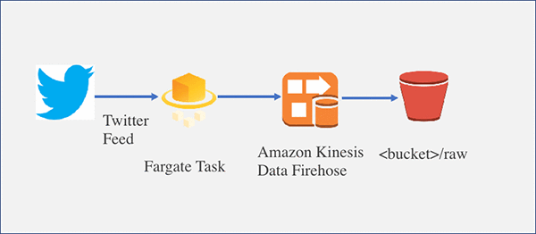
Our focus for this blog post is to move the Twitter stream producer app from running in an EC2 instance to running in containers managed by Fargate.

We’ll start by creating a Docker image that has our code for the Twitter feed reader application, plus all of its dependencies. After we have the Docker image, we’ll upload and register this image to ECR, which serves as a repository for Docker images. With the image registered in ECR, we are going to create a task definition, which describes the configuration we want to set for running our Docker container in the Fargate service. Finally, we are going to run the task and test our app.

Prerequisites

  1. Go to the previous blog post and follow the instructions found there. The high level steps are:
    1. Launching the AWS CloudFormation template. When you launch the template you need to provide the Twitter API configuration parameters.
    2. After the CloudFormation stack is created go to the AWS Management Console, search for the stack and choose the Resources Take note of the Physical ID of the IngestionFirehoseStream resource. It will be something like: SocialMediaAnalyticsBlogPo-IngestionFirehoseStream-<ID>
    3. Setting up S3 Notification – Call Amazon Translate/Comprehend from new Tweets.
    4. Start the Twitter stream producer. This is the application that is running in an EC2 instance.
    5. Create the Athena tables. This is done by running four different SQL statements.
    6. (optional – recommended) Building Amazon QuickSight dashboards.
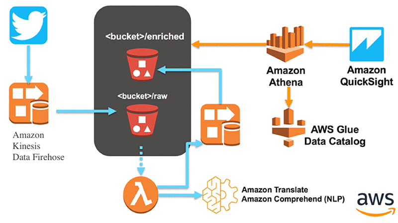
      After you complete all the steps you should have following architecture deployed on your environment:
  2. Configure an environment where you can run AWS CLI and Docker commands. You can launch an EC2 instance and install Docker or you can use AWS Cloud9, which comes with Docker. We used an EC2 instance and installed Docker in it. If you decide to go with the EC2 option, you’ll need to create an IAM role and attach it to the instance.
    {
        "Version": "2012-10-17",
        "Statement": [
            {
                "Sid": "VisualEditor0",
                "Effect": "Allow",
                "Action": [
                    "ssm:PutParameter",
                    "firehose:*",
                    "iam:CreateRole",
                    "ecr:*",
                    "iam:AttachRolePolicy",
                    "ssm:GetParameter"
                ],
                "Resource": "*"
            }
        ]
    }
    

    We are going to refer this environment as the “Dev Environment” in the following steps. We will use the Dev Environment to create our Docker image and register the image with the ECR service. This environment will need permission to use Amazon Kinesis Data Firehose, ECR, and IAM APIs.

    Note: You need to install the AWS CLI on the Docker environment. For AWS CLI installation, refer this page.

 Step 1: Create the Docker image

To create the Docker image, first we need to create a Dockerfile. A Dockerfile is a manifest that describes the base image to use for your Docker image and what you want installed and running on it. For more information about Dockerfiles, go to the Dockerfile Reference. In our case, we want to create a Docker image that we use to instantiate containers that run Node applications. In particular, we want to run our Twitter stream producer node app.

  1. Choose a directory in the Docker environment and perform the following steps in that directory. I used /home/ec2-user directory to perform the following steps.
  2. Download the application code to our Dev Environment. When you executed the instructions in the prerequisites section 1.a, a CloudFormation template was used to create a stack called SocialMediaAnalyticsBlogPost. This stack configures the EC2 instance with the Twitter stream producer app. If you open the CloudFormation file and go to the EC2 configuration section (line 229 in the template), you will find that the application code was copied from an Amazon S3 bucket to the EC2 instance. We want to copy the same code to our Dev Environment. Use the following command:
    mkdir SocialAnalyticsReader
    
    cd socialAnalyticsReader
    
    wget https://s3.amazonaws.com/serverless-analytics/SocialMediaAnalytics-blog/SocialAnalyticsReader.tar
    
    tar -xf SocialAnalyticsReader.tar

  3. Now we are going to do a small refactor on the SocialAnalyticsReader app. The Node application is currently designed to read the Twitter API credentials from a configuration file. We want to avoid this approach after the application runs on a container. A better way is to store the configuration settings on a service like AWS Systems Manager Parameter Store. Extracting the configuration settings increases the flexibility and reusability of our container image. For example, it allows us to change the configuration values for the application without the need of rebuilding the Docker image.Replace the contents of the following files:twitter_stream_producer_app.js
    'use strict';
    
    
    var AWS = require('aws-sdk');
    var config = require('./config');
    var producer = require('./twitter_stream_producer');
    
    // var kinesis = new AWS.Kinesis({region: config.kinesis.region});
    var kinesis_firehose = new AWS.Firehose({apiVersion: '2015-08-04', region: config.region});
    // console.log(kinesis_firehose.listDeliveryStreams());
    
    var params = {
      Name: '/twitter-reader/aws-config', /* required */
      WithDecryption: false
    };
    
    var config_from_parameter_store;
    var ssm = new AWS.SSM({region: config.region});
    var request = ssm.getParameter(params);
    var promise = request.promise();
    
    promise.then(
       function(data){
          console.log('promise then:',data.Parameter.Value);
         // global.twitter_config = data.Parameter.Value;
          producer(kinesis_firehose, data.Parameter.Value).run();
       },
       function(error){
            console.log(error);
       });
    

    twitter_stream_producer.js

    'use strict';
    
    var config = require('./config');
    //var twitter_config = require('./twitter_reader_config.js');
    var Twit = require('twit');
    var util = require('util');
    var logger = require('./util/logger');
    
    function twitterStreamProducer(firehose, twitter_config_str) {
      var twitter_config = JSON.parse(twitter_config_str);
      var log = logger().getLogger('producer');
      var waitBetweenPutRecordsCallsInMilliseconds = config.waitBetweenPutRecordsCallsInMilliseconds;
      var T = new Twit(twitter_config.twitter)
    
      function _sendToFirehose() {
    
        var stream = T.stream('statuses/filter', { track: twitter_config.topics , language: twitter_config.languages });
    
    
        var records = [];
        var record = {};
        var recordParams = {};
        stream.on('tweet', function (tweet) {
                    var tweetString = JSON.stringify(tweet)
                    recordParams = {
                      DeliveryStreamName: twitter_config.kinesis_delivery,
                      Record: {
                        Data: tweetString +'n'
                      }
                    };
                  firehose.putRecord(recordParams, function(err, data) {
                    if (err) {
                      console.log(err);
                    }
                  });
            }
        );
      }
    
    
      return {
        run: function() {
          log.info(util.format('Configured wait between consecutive PutRecords call in milliseconds: %d',
              waitBetweenPutRecordsCallsInMilliseconds));
            _sendToFirehose();
          }
      }
    }
    
    module.exports = twitterStreamProducer;
    

    If you compare the new files with the original version, you will notice that only a few lines of code were changed. In summary, our application will now use the AWS Node SDK to retrieve configuration settings from AWS Systems Manager Parameter store instead of retrieving them from a config file. For additional information on recommended approaches for handling configuration and secrets on containers, we recommend this blog post.

  4. Navigate back to /home/ec2-user directory and create a file called Dockerfile (case sensitive) with the following content:
    FROM amazonlinux:2017.09
    RUN curl -o- https://raw.githubusercontent.com/creationix/nvm/v0.32.0/install.sh | bash 
            && . ~/.nvm/nvm.sh 
            && nvm install 8.10.0
    ENV PATH /root/.nvm/versions/node/v8.10.0/bin:$PATH
    WORKDIR /home/ec2-user
    RUN mkdir twitterApp
    COPY ./SocialAnalyticsReader/ /home/ec2-user/twitterApp
    RUN chmod ugo+x /home/ec2-user/*
    USER root
    WORKDIR /home/ec2-user/twitterApp
    	 ENTRYPOINT ["node","twitter_stream_producer_app.js"]

  5. After completing these steps, your directory structure will look like this:

Step 2: Build the Docker image

Build the Docker image by running this command from the directory where you created the Dockerfile in the Docker environment in the previous step (I ran it from /home/ec2-user directory):

docker build –t tweetreader .

Output: It installs various packages and sets environment variables as part of building the image from the Dockerfile. The steps 5 to 10 from the Dockerfile should produce an output similar to the following:

Step 5/8 : COPY ./SocialAnalyticsReader/ /home/ec2-user/twitterApp/
 ---> Using cache
 ---> 04d0088db623
Step 6/8 : RUN chmod ugo+x /home/ec2-user/*
 ---> Running in 5e4d9cc10239
Removing intermediate container 5e4d9cc10239
 ---> 5d7d7328cb93
Step 7/8 : USER root
 ---> Running in 893f1653c200
Removing intermediate container 893f1653c200
 ---> dfc016c8e4a7
Step 8/8 : ENTRYPOINT ["node","twitterApp/twitter_stream_producer_app.js"]
 ---> Running in a839a2139689
Removing intermediate container a839a2139689
 ---> ba5ede432da0
Successfully built ba5ede432da0
Successfully tagged tweetreader:latest

Step 3: Push the Docker image to Amazon Elastic Container Registry (ECR)

Now we are going to upload the Docker image we just built to Amazon Elastic Container Registry (ECR), a fully-managed Docker container registry that makes it easy for developers to store, manage, and deploy Docker container images. Amazon ECR is integrated with Amazon Elastic Container Service (ECS), simplifying your development to production workflow.

Perform the following steps in the Dev Environment.

  1. Run the following aws configure command and set the default Region to be us-east-1.
    aws configure set default.region us-east-1

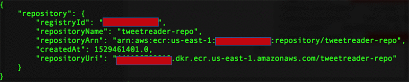
  2. Create an Amazon ECR repository using this command (note the repositoryUri in the output):
    aws ecr create-repository --repository-name tweetreader-repo

Output:

  1. Tag the tweetreader image with the repositoryUri value from the previous step using this command:
    docker tag tweetreader:latest aws_account_id.dkr.ecr.us-east-1.amazonaws.com/ tweetreader-repo

  2. Get the Docker login credentials using the following command:
    aws ecr get-login --no-include-email

  3. Run the Docker login command returned from the previous step. If the command is successful, you will get a message “Login Succeeded.”
  4. Push the Docker image to Amazon ECR with the repositoryUri from step 1 using this command:
    docker push aws_account_id.dkr.ecr.us-east-1.amazonaws.com/tweetreader-repo

Step 4: Store configuration information in AWS Systems Manager Parameter Store

Now we are going to store application configuration information in AWS Systems Manager Parameter Store, which provides hierarchical storage for configuration data management and secrets management. You can store data such as passwords, database strings, and license codes as parameter values. By storing our configuration parameters outside the container we improve the security posture by separating this data from the code and enabling us to control and audit access at granular levels. 

  1. Go to the AWS Management Console and navigate to the AWS Systems Manager console.
  2. In the navigation pane at the left, scroll to the bottom and choose Parameter Store and then choose create parameter at the top right.
    For name use : /twitter-reader/aws-configFor type: select StringFor Value:

    { "twitter": {
     "consumer_key": "VAL1", 
    "consumer_secret": "VAL2", 
    "access_token": "VAL3", 
    "access_token_secret": "VAL4" }, 
    "topics": ["AWS", "VPC", "EC2", "RDS", "S3", "ECSSSS"], 
    "languages": ["en", "es", "de", "fr", "ar", "pt"],
     "kinesis_delivery": "VAL5" }

    • Update the placeholders VAL1 through VAL4 with the values corresponding to your Twitter API credentials.
    • Update the placeholder VAL5 with the value captured in the Prerequisites section step b IngestionFirehoseStream physical ID.
    • The value will be something like SocialMediaAnalyticsBlogPo-IngestionFirehoseStream-<value>
    • Choose Create Parameter.

Step 5: Create Fargate task definition and cluster

Now we are going to configure a task for Amazon ECS using AWS Fargate as the launch type. The Fargate launch type allows you to run your containerized applications without the need to provision and manage the backend infrastructure. 

  1. Create a text file called trustpolicyforecs.json with the following content in the DevEnvironment:
    {
      "Version": "2012-10-17",
      "Statement": [
        {
          "Effect": "Allow",
          "Principal": {
            "Service": "ecs-tasks.amazonaws.com"
          },
          "Action": "sts:AssumeRole"
        }
      ]
    }

  2. Create a role called AccessRoleForTweetReaderfromFG using the following command in the DevEnvironment:
    aws iam create-role --role-name AccessRoleForTweetReaderfromFG --assume-role-policy-document file://trustpolicyforecs.json

  3. Attach Kinesis Data Firehose and Systems Manager IAM policies to the role created in step 2 using the following commands in the DockerEnvironment:
    aws iam attach-role-policy --policy-arn arn:aws:iam::aws:policy/AmazonKinesisFirehoseFullAccess --role-name AccessRoleForTweetReaderfromFG
    
    aws iam attach-role-policy --policy-arn arn:aws:iam::aws:policy/AmazonSSMReadOnlyAccess --role-name AccessRoleForTweetReaderfromFG

    AccessRoleForTweetReaderfromFG is the IAM role that will be assumed by the task running on ECS. Our task is running the Node application and only needs IAM policies to write records to Kinesis Data Firehose and read configuration information from AWS Systems Manager Parameter Store.

  4. In the Amazon ECS console, choose Repositories and select the tweetreader-repo repository that was created in the previous step. Copy the Repository URI.
  5. Choose Task Definitions and then choose Create New Task Definition.
  6. Select launch type compatibility as FARGATE and click Next Step.
  7. In the create task definition screen, do the following:
    • In Task Definition Name, type tweetreader-task
    • In Task Role, choose AccessRoleForTweetReaderfromFG
    • In Task Memory, choose 2GB
    • In Task CPU, choose 1 vCPU
    • Choose Add Container under Container Definitions. On the Add Container page, do the following:
      • Enter Container name as tweetreader-cont
      • Enter Image URL copied from step 1
      • Enter Memory Limits as 128 and choose Add.

    Note: Select TaskExecutionRole as “ecsTaskExecutionRole” if it already exists. If not, select Create new role and it will create “ecsTaskExecutionRole” for you.

  8. Choose the Create button on the task definition screen to create the task. It will successfully create the task, execution role and Amazon CloudWatch Logs groups.
  9. In the Amazon ECS console, choose Clusters and create cluster. Select template as “Networking only, Powered by AWS Fargate” and chooose the next step.
  10. Enter cluster name as tweetreader-cluster and choose Create.

Step 6: Start the Fargate task and verify the application       

  1. In the Amazon ECS console, go to Task Definitions, select the tweetreader-task, choose Actions, and then choose Run Task.
  2. On the Run Task page, for Launch Type select Fargate, for Cluster select tweetreader-cluster, select Cluster VPC and Subnets values, and then choose Run Task.
  3. To test the application, choose the running task in the Fargate console. Go to the logs tab and verify there is nothing there. This means the node application is running and no errors occurred. After you have verified that the Fargate task does not have any error logs, navigate to the Amazon S3 console and go to the bucket that was created as part of the CloudFormation template in the original blog post. You will see a folder called raw. Check the contents of this folder. It should have the data sent from our Twitter feed reader app to serverless processing flow (Amazon Kinesis Data Firehose, Amazon Lex, Amazon Translate, Amazon Athena )

Conclusion

Congratulations! You have successfully ‘containerized’ an application that was previously running on an EC2 instance. Furthermore, you are running the container with Amazon ECS and AWS Fargate so you don’t need to provision or manage any EC2 instances. You can also tweak the task definition configuration in AWS Fargate by tuning the amount of memory, CPU, and concurrent executions your task might need.

For more information about working with ECS and Fargate, see the AWS Fargate documentation.


About the Authors

Raja Mani is a Solution Architect supporting AWS partners. He is interested in Serverless development, DevOps, Containers, Big Data and Machine Learning. He is helping AWS partners to architect the enterprise-grade Amazon Web Services Solutions for their customers.



Luis Pineda is a Partner Solutions Architect at Amazon Web Services based in Chicago. He works with our partners and customers to solve business problems using AWS. Outside of work, Luis enjoys being outdoors, running, cycling and soccer.


Anomaly detection on Amazon DynamoDB Streams using the Amazon SageMaker Random Cut Forest algorithm

Have you considered introducing anomaly detection technology to your business? Anomaly detection is a technique used to identify rare items, events, or observations which raise suspicion by differing significantly from the majority of the data you are analyzing.  The applications of anomaly detection are wide-ranging including the detection of abnormal purchases or cyber intrusions in banking, spotting a malignant tumor in an MRI scan, identifying fraudulent insurance claims, finding unusual machine behavior in manufacturing, and even detecting strange patterns in network traffic that could signal an intrusion.

There are many commercial products to do this, but you can easily implement an anomaly detection system by using Amazon SageMaker, AWS Glue, and AWS Lambda. Amazon SageMaker is a fully-managed platform to help you quickly build, train, and deploy machine learning models at any scale. AWS Glue is a fully-managed ETL service that makes it easy for you to prepare your data/model for analytics. AWS Lambda is a well-known a serverless real-time platform. Using these services, your model can be automatically updated with new data, and the new model can be used to alert for anomalies in real time with better accuracy.

In this blog post I’ll describe how you can use AWS Glue to prepare your data and train an anomaly detection model using Amazon SageMaker. For this exercise, I’ll store a sample of the NAB NYC Taxi data in Amazon DynamoDB to be streamed in real time using an AWS Lambda function.

The solution that I describe provides the following benefits:

  • You can make the best use of existing resources for anomaly detection. For example, if you have been using Amazon DynamoDB Streams for disaster recovery (DR) or other purposes, you can use the data in that stream for anomaly detection. In addition, stand-by storage usually has low utilization. The data in low awareness can be used for training data.
  • You can automatically retrain the model with new data on a regular basis with no user intervention.
  • You can make it easy to use the Random Cut Forest built-in Amazon SageMaker algorithm. Amazon SageMaker offers flexible distributed training options that adjust to your specific workflows in a secure and scalable environment.

Solution architecture

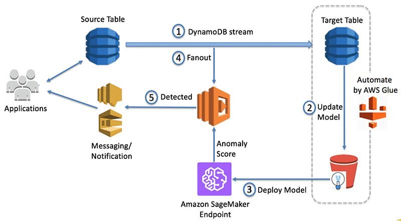
The following diagram shows the overall architecture of the solution.

The steps that data follows through the architecture are as follows:

  1. Source DynamoDB captures changes and stores them in a DynamoDB stream.
  2. AWS Glue job regularly retrieves data from target DynamoDB table and runs a training job using Amazon SageMaker to create or update model artifacts on Amazon S3.
  3. The same AWS Glue job deploys the updated model on the Amazon SageMaker endpoint for real-time anomaly detection based on Random Cut Forest.
  4. AWS Lambda function polls data from the DynamoDB stream and invokes the Amazon SageMaker endpoint to get inferences.
  5. The Lambda function alerts user applications after anomalies are detected.

This blog post consists of two sections. The first section, “Building the auto-updating model,” explains how the previous steps 1, 2, and 3 can be automated using AWS Glue. All of the sample scripts in this section run in one AWS Glue job. The second section, “Detecting anomalies in real time,” shows how the AWS Lambda function processes previous steps 4 and 5 for anomaly detection.

Building the auto-updating model

This section explains how AWS Glue reads a DynamoDB table and automatically trains and deploys a model of Amazon SageMaker. I assume that the DynamoDB stream is already enabled and DynamoDB items are being written to the stream. If you have not set these up yet, you can reference these documents for more information: Capturing Table Activity with DynamoDB Streams, DynamoDB Streams and AWS Lambda Triggers, and Global Tables.

In this example, a DynamoDB table (“taxi_ridership”) in the us-west-2 Region is replicated to another DynamoDB table with same name in us-east-1 Region using the Global Tables of DynamoDB.

Create an AWS Glue job and prepare data

To prepare data for model training, we’ll store our data in DynamoDB. The AWS Glue job retrieves data from the target DynamoDB table by using create_dynamic_frame_from_options() with a dynamodb connection_type argument. While you pull data from DynamoDB, we recommend that you choose only the necessary columns for model training and write them into Amazon S3 as CSV files.  You can do this by using the ApplyMapping.apply() function in AWS Glue. In this example, only the transaction_id and ridecount columns are mapped.

In addition, when you run the write_dynamic_frame.from_options function, you need to add this option,  format_options = {"writeHeader": False , "quoteChar": "-1" }, because the column’s name and double quotation marks (‘”‘) are not necessary for model training.

Finally, the AWS Glue job should be created in the same Region (for this blog post it’s us-east-1 ) where the DynamoDB table resides. For more information on creating an AWS Glue job. See Adding Jobs in AWS Glue.

import sys
from awsglue.transforms import *
from awsglue.utils import getResolvedOptions
from pyspark.context import SparkContext
from awsglue.context import GlueContext
from awsglue.job import Job

## @params: [JOB_NAME]
args = getResolvedOptions(sys.argv, ['JOB_NAME'])
 
sc = SparkContext()
glueContext = GlueContext(sc)
spark = glueContext.spark_session
job = Job(glueContext)
job.init(args['JOB_NAME'], args)

my_region  = '<region name>'
my_bucket = '<bucket name>'
my_project = '<project name>'
my_train_data = "s3://{}/{}/taxi-ridership-rawdata/".format(my_bucket ,  my_project )
my_dynamodb_table = "taxi_ridership"

## Read raw(source) data from target DynamoDB 
raw_data_dyf = glueContext.create_dynamic_frame_from_options("dynamodb", {"dynamodb.input.tableName" : my_dynamodb_table , "dynamodb.throughput.read.percent" : "0.7" } , transformation_ctx="raw_data_dyf" )
 
## Write necessary columns into S3 as CSV format for creating Random Cut Forest(RCF)  model  
selected_data_dyf = ApplyMapping.apply(frame = raw_data_dyf, mappings = [("transaction_id", "string", "transaction_id", "string"), ("ridecount", "string", "ridecount", "string")], transformation_ctx = "selected_data_dyf")
datasink = glueContext.write_dynamic_frame.from_options(frame=selected_data_dyf , connection_type="s3", connection_options={ "path": my_train_data }, format="csv", format_options = {"writeHeader": False , "quoteChar": "-1" }, transformation_ctx="datasink")

This AWS Glue job writes CSV files in the specified path on Amazon S3 ( “s3://<bucket name>/<project name>/taxi-ridership-rawdata/” ).

Run training job and update model

After the data is prepared, you can run a training job on Amazon SageMaker. To submit the training job to Amazon SageMaker the boto3 package, which is automatically bundled with your AWS Glue ETL script, should be imported. This enables you to use the low-level SDK for Python in the AWS Glue ETL script. To learn more about how to create a training job, see Create a Training Job.

The create_training_job function creates model artifacts on the S3 path you specified. Those model artifacts are required for creating the model in the next step.

## Execute training job with CSV data and create model artifacts for RCF
import boto3
from time import gmtime, strftime

sagemaker = boto3.client('sagemaker', region_name= my_region)
job_name = 'randomcutforest-' + strftime("%Y-%m-%d-%H-%M-%S", gmtime())
sagemaker_role = "arn:aws:iam::<account id>:role/service-role/<AmazonSageMaker-ExecutionRole-Name>"

containers = {
    'us-west-2': '174872318107.dkr.ecr.us-west-2.amazonaws.com/randomcutforest:latest',
    'us-east-1': '382416733822.dkr.ecr.us-east-1.amazonaws.com/randomcutforest:latest',
    'us-east-2': '404615174143.dkr.ecr.us-east-2.amazonaws.com/randomcutforest:latest',
    'eu-west-1': '438346466558.dkr.ecr.eu-west-1.amazonaws.com/randomcutforest:latest'}

image = containers[my_region]
artifacts_location = 's3://{}/{}/artifacts'.format(my_bucket , my_project )
print('myINFO : training artifacts will be uploaded to: {}'.format(artifacts_location))

create_training_params = 
{
    "AlgorithmSpecification": { "TrainingImage": image, "TrainingInputMode": "File" },
    "RoleArn": sagemaker_role, "OutputDataConfig": {"S3OutputPath": artifacts_location },
    "ResourceConfig": { "InstanceCount": 2, "InstanceType": "ml.c4.xlarge", "VolumeSizeInGB": 50 },
    "TrainingJobName": job_name,
    "HyperParameters": { "num_samples_per_tree": "200", "num_trees": "50", "feature_dim": "2" },
    "StoppingCondition": { "MaxRuntimeInSeconds": 60 * 60 },
    "InputDataConfig": [
        {
            "ChannelName": "train",
            "ContentType": "text/csv;label_size=0",
            "DataSource": {
                "S3DataSource": {"S3DataType": "S3Prefix", "S3Uri": my_train_data, "S3DataDistributionType": "ShardedByS3Key" } 
            },
            "CompressionType": "None",
            "RecordWrapperType": "None"
        }
    ]
}

sagemaker.create_training_job(**create_training_params)
status = sagemaker.describe_training_job(TrainingJobName=job_name)['TrainingJobStatus']
print('myINFO : Status of {} traning job ==>  {}'.format(job_name , status ))
 
try:
    sagemaker.get_waiter('training_job_completed_or_stopped').wait(TrainingJobName=job_name)
finally:
    status = sagemaker.describe_training_job(TrainingJobName=job_name)['TrainingJobStatus']
    print("myINFO : Training job ended with status: " + status)
    if status == 'Failed':
        message = sagemaker.describe_training_job(TrainingJobName=job_name)['FailureReason']
        print('myINFO : Training failed with the following error: {}'.format(message))
        raise Exception('Training job failed')

## Create Model from model artifacts 
model_name=job_name
print("myINFO : Model name - {}".format(model_name))

info = sagemaker.describe_training_job(TrainingJobName=job_name)
model_data = info['ModelArtifacts']['S3ModelArtifacts']
primary_container = {'Image': image, 'ModelDataUrl': model_data }

create_model_response = sagemaker.create_model(
    ModelName = model_name,
    ExecutionRoleArn = sagemaker_role,
    PrimaryContainer = primary_container)
print("myINFO : Created Model ARN : {}".format( create_model_response['ModelArn']))

You can see a new model name with date format on the Amazon SageMaker console after model creation is successful.

Execute batch transform and obtain cut-off score

We can now use this trained model to compute anomaly scores for each of the training data points. As the amount of data to work with is big, I decided to use Amazon SageMaker Batch Transform. Batch transform uses a trained model to get inferences for an entire dataset in Amazon S3, and saves the inferences in an S3 bucket that you specify when you create a batch transform job.

After getting the inferences (=anomaly scores) on each data point, we need to obtain a score_cutoff value to be used for real-time anomaly detection. To make it simple, I used a standard technique for classifying anomalies. Anomaly scores outside three standard deviations from the mean score are considered anomalous.

## Execute Batch Transform in order to calculate anomaly scores and the value of score cutoff.
## score cutoff will be used in Lambda function in real time to identify anomalous transaction 
import time
batch_job_name = 'Batch-Transform-' + strftime("%Y-%m-%d-%H-%M-%S", gmtime())
batch_output = "s3://{}/{}/batch_output/".format(my_bucket , my_project )

request = {
        "TransformJobName": batch_job_name,
        "ModelName": model_name,
        "MaxConcurrentTransforms": 1, 
        "TransformOutput": { "S3OutputPath": batch_output },
        "TransformInput" : { 
            "ContentType": "text/csv;label_size=0",
             "DataSource" : { 
                 "S3DataSource": { "S3DataType": "S3Prefix", "S3Uri": my_train_data } 
             }
        }, 
       "TransformResources": { "InstanceType": "ml.m4.xlarge","InstanceCount": 1  } 
}
response = sagemaker.create_transform_job(**request)

batch_status = 'InProgress'
while batch_status == 'InProgress':
    batch_status = sagemaker.describe_transform_job( TransformJobName=batch_job_name)['TransformJobStatus']
    print("myINFO : Batch job {} in Progress ".format( batch_job_name ))
    time.sleep(10)
if batch_status == 'Failed':
    message = sagemaker.describe_transform_job(TransformJobName=batch_job_name)['FailureReason']
    print('myINFO : Transforming job failed with the following error: {}'.format(message))
    raise Exception('Transforming job failed')

## Calculate score_cutoff from the result of Batch-Transform 
from pyspark.sql.functions import mean, stddev
from decimal import Decimal
all_scores_dfy = glueContext.create_dynamic_frame_from_options("s3", {'paths': [ batch_output ]}, format="json", transformation_ctx = "all_scores_dfy" ).toDF()
score_mean = all_scores_dfy.agg(mean(all_scores_dfy["score"]).alias("mean")).collect()[0]["mean"]
score_stddev = all_scores_dfy.agg(stddev(all_scores_dfy["score"]).alias("stddev")).collect()[0]["stddev"]
score_cutoff = Decimal( str( score_mean + 3*score_stddev ) ) 
print("myINFO : RFC score cutoff : {}".format( score_cutoff))

The history of the batch transform job can be found in the Batch transform jobs menu on the Amazon SageMaker console.

Deploy model and update cut-off score

The final step in the AWS Glue ETL script is to deploy the updated model on the Amazon SageMaker endpoint and upload the obtained score_cutoff value in the DynamoDB table for real-time anomaly detection. The Lambda function queries this score_cutoff value on DynamoDB to compare it with anomaly scores of new transactions.

## Create Endpoint Configuration for realtime service 
endpoint_config_name = 'randomcutforest-endpointconfig-' + strftime("%Y-%m-%d-%H-%M-%S", gmtime()) 
create_endpoint_config_response = sagemaker.create_endpoint_config(
    EndpointConfigName = endpoint_config_name,
    ProductionVariants=[{ 'InstanceType':'ml.m4.xlarge', 'InitialInstanceCount':1, 'ModelName':model_name, 'VariantName':'AllTraffic'}]
)
print("myINFO : Endpoint Config Arn:  " + create_endpoint_config_response['EndpointConfigArn'] )


##  Create/Update Endpoint with new configuration that has updated model. 
endpoint_name = 'randomcutforest-endpoint'
endpoint_status = ""
try:
    endpoint_status = sagemaker.describe_endpoint(EndpointName=endpoint_name)['EndpointStatus']
except Exception as e : 
    endpoint_status = "NotInService"
print("myINFO : randomcutforest-endpoint Status: " + status)

if endpoint_status == 'InService':
    update_endpoint_response = sagemaker.update_endpoint( EndpointName=endpoint_name, EndpointConfigName=endpoint_config_name)
    try:
        sagemaker.get_waiter('endpoint_in_service').wait(EndpointName=endpoint_name)
    finally:
        resp = sagemaker.describe_endpoint(EndpointName=endpoint_name) 
        status = resp['EndpointStatus']
        print("myINFO : Update endpoint {} ended with {} status: ".format( resp['EndpointArn'] , status ) )         
        if status != 'InService':
            message = sagemaker.describe_endpoint(EndpointName=endpoint_name)['FailureReason']
            print('myINFO : Endpoint update failed with the following error: {}'.format(message))
            raise Exception('Endpoint update did not succeed')
else:
    create_endpoint_response = sagemaker.create_endpoint( EndpointName=endpoint_name, EndpointConfigName=endpoint_config_name)
    try:
        sagemaker.get_waiter('endpoint_in_service').wait(EndpointName=endpoint_name)
    finally:
        resp = sagemaker.describe_endpoint(EndpointName=endpoint_name) 
        status = resp['EndpointStatus']
        print("myINFO : Create endpoint {} ended with {} status: ".format( resp['EndpointArn'] , status ) )         
        if status != 'InService':
            message = sagemaker.describe_endpoint(EndpointName=endpoint_name)['FailureReason']
            print('myINFO : Endpoint creation failed with the following error: {}'.format(message))
            raise Exception('Endpoint creation did not succeed')

            
## Add the score_cutoff value into DynamoDB 
## score_cutoff will be queried by Lambda function for real time abnormal detection
dynamodb_table = boto3.resource('dynamodb', region_name= my_region).Table('anomaly_cut_off')
dynamodb_table.put_item(Item= {'data_kind': my_dynamodb_table ,'update_time':  strftime("%Y%m%d%H%M%S", gmtime()), 'score_cutoff': score_cutoff })
print('myINFO : New score_cutoff value has been updated in DynamoDB table.')
    
## Delete Temporary data to save cost. 
s3 = boto3.resource('s3').Bucket(my_bucket ) 
s3.objects.filter(Prefix="{}/taxi-ridership-rawdata".format(my_project)).delete()
s3.objects.filter(Prefix="{}/batch_output".format(my_project)).delete()
print('myINFO : Temporary S3 objects have been deleted.')

## End job 
job.commit()

Now the Amazon SageMaker endpoint is created, and the AWS Glue job has been completed. You can check the detailed log of the AWS Glue job by choosing the Logs link in the AWS Glue console.

The score_cutoff value is stored in a DynamoDB table whose partition key is taxi-ridership and whose range key is a latest update time.

Schedule the AWS Glue job

Those previous scripts run in the same AWS Glue job and AWS Glue supports a time-based schedule by creating a trigger. You can retrain model with new data on regular basis if you define a time-based schedule and associate it with your job.  I do not think the model should be updated too frequently.  Weekly or bi-weekly renewal should be enough.

Detecting anomalies in real time

This section discusses how to detect anomalous transactions in real time from an AWS Lambda function. You need to create an AWS Lambda function to poll the DynamoDB stream. While you create the AWS Lambda function, you can use the “dynamodb-process-stream-python3” blueprint for quick implementation. The Lambda function with the blueprint can be integrated with the DynamoDB table that you specify. The blueprint provides the basic Lambda code.

Get an anomaly score on each data point

I’ll briefly explain the code in the Lambda function. It filters only INSERT and MODIFY events because they are new data.  The Lambda function adds them into instances array in order to get inferences for an entire events in the array. The Amazon SageMaker Random Cut Forest algorithm accepts multiple records as input requests and return multi-record inferences to support a mini-batch predictions. To learn more, see Common Data Formats—Inference.

import json
import boto3
from boto3.dynamodb.conditions import Key, Attr

print("Starting Lambda Function.... ")
sagemaker = boto3.client('sagemaker-runtime', region_name ='<region name>' )
dynamodb_table = boto3.resource('dynamodb', region_name='us-east-1').Table('anomaly_cut_off')

def lambda_handler(event, context):
    #print("Received event: " + json.dumps(event, indent=2))
    transaction_data = {} # key : transaction_id / value : ridecount
    
    for record in event['Records']:
        ## filter only INSERT or MODIFY event and add to "transaction_data" dictionary 
        if record['eventName'] == "INSERT" or record['eventName'] == "MODIFY":
            transaction_id = record['dynamodb']['NewImage']['transaction_id']['S']
            ridecount = record['dynamodb']['NewImage']['ridecount']['S']
            transaction_data[transaction_id] = ridecount
    print( "transaction_data: " + str(transaction_data )) 
    
    features=[]  
    features_dic={}   
    instances=[]
    instances_dic={}  # example, {'instances': [{'features': ['10231', '3837']}, {'features': ['10232', '10844']}]}
    for key in transaction_data.keys():
        features.append(key)
        features.append(transaction_data[key])
        features_dic["features"] = features
        instances.append(features_dic)
        features=[]
        features_dic={}
    instances_dic["instances"] = instances
    transaction_json = json.dumps(instances_dic)  # To make argument format for invoke_endpoint method.

Alert anomalous transaction

An array of features can be submitted to the sagemaker.invoke_endpoint function. It returns an array of scores corresponding to each feature in the instances array. We can compare each score in response to the latest value of score_cutoff retrieved from the DynamoDB table. If the anomaly score of a new transaction is larger than the value of score_cutoff, that transaction is considered to be anomalous. Then the Lambda function will alert the user application.

    response = sagemaker.invoke_endpoint( EndpointName='randomcutforest-endpoint', Body=transaction_json ,  ContentType='application/json' )
    scores_result = json.loads(response['Body'].read().decode())
    print("Result score : "+ str(scores_result))  # return an array of score 
    
    response = dynamodb_table.query(
              Limit = 1,
              ScanIndexForward = False,
              KeyConditionExpression=Key('data_kind').eq('taxi_ridership') & Key('update_time').lte('99990000000000')
           )
    socre_cutoff = response['Items'][0]['score_cutoff'] 
    print("socre cutoff : " + str(socre_cutoff) )       
    
    for index in range(len(scores_result['scores'])):
        if scores_result['scores'][index]['score'] > socre_cutoff:
            print("Detected abnormal transaction ID : {} , Ridecount : {}".format(instances[index]['features'][0], instances[index]['features'][1]   ))
            ## Add your codes to send a notification
            
    return 'Successfully processed {} records.'.format(len(event['Records']))

The following is an example of an output log in Amazon CloudWatch. Two transactions (10231 and 21101) were created  in DynamoDB, and those transaction triggered a Lambda function as new events. The anomaly score of transaction of 21101 is 3.6189932108. That is larger than the cut-off value (1.31462299965) in the DynamoDB table, so the transaction is detected to be anomalous.

Conclusion

In this blog post, I introduced an example of how to build an anomaly detection system on Amazon DynamoDB Streams by using Amazon SageMaker, AWS Glue, and AWS Lambda.

In addition, you can adapt this example to your specific use case because AWS Glue is very flexible based on user’s script and continues to add new data source. Other kinds of data sources and streams can be applied to this architecture because AWS Lambda function also works with many other AWS streaming services.

Finally, I hope this post helps you reduce business risks and save cost while adopting anomaly detection system.


About the Author

Yong Seong Lee is a Cloud Support Engineer for AWS Big Data Services. He is interested in every technology related to Big Data/Data Analysis/Machine Learning and helping customers who have difficulties in using AWS services. His motto is “Enjoy life, be curious and have maximum experience.”


Announcing the Winners of the 2018 AWS AI Hackathon

We’re excited to announce the winners of the 2018 AWS AI Hackathon.  Horacio Canales has won first place with his “Second Alert” project. This project enables users from around the world to identify missing persons, including human trafficking victims, children too young to remember their family members’ names, and mentally handicapped individuals. Horacio built the solution using image analysis, text analysis, and conversational agents with Amazon Rekognition, Amazon Comprehend, and Amazon Lex. In recognition for his contribution, Horacio will receive $5,000 USD and $2,500 in AWS Credits.

We want to thank all of the participating developers from around the world for their time and creativity during the 2018 AWS AI Hackathon. In this hackathon, we challenged developers to build intelligent applications using pre-trained machine learning computer vision, natural language processing, speech recognition, text-to-speech, and machine translation API services. Last week our judges determined three winners from more than 900 submissions.

Developers submitted projects aimed at applying artificial intelligence to solve problems in ecommerce, health, entertainment, and much more. Our judges reviewed submissions based on the quality, creativity, and originality of the idea; implementation of the idea, including how well AWS machine learning services were leveraged by the developer; and the potential impact of the idea, such as how the solution can be widely useful. Our panel of judges included machine learning and open source experts from across AWS:

Congratulations to our winners!

1st Place | $5,000 USD and $2,500 in AWS Credits: Second Alert, by Horacio Canales. Horacio was motivated to help identify missing persons using facial recognition. AWS services used include Amazon Rekognition, Amazon Comprehend, Amazon Lex, and AWS Lambda.

2nd Place | $3,000 USD and $1,500 in AWS Credits: Mobu, by Yosun Chang and Luannie Dang. Yosun built an “empathy-powered movie buddy robot” that recommends movies using chat, image recognition, and a person’s mood—by determining user happiness through facial analysis. AWS services used include Amazon Rekognition, Amazon Lex, and AWS Lambda.

3rd Place | $2,000 USD and $1,000 in AWS Credits: Lab monitor, by Kitson Cheung, Cyrus Wong Chun Yin, Kwok Tung Chan, Chun Long Kwan, Mei Ching Law, Fung Lam Jacqueline Wu, Mike Ng, and Man Ting Ma. This team built an application that helps students stay focused during technical lab classes. AWS services used include Amazon Rekognition, Amazon Polly, Amazon Lex and AWS Lambda. 

Honorable Mentions

We also recognize these four submissions in no particular order, with $300 in AWS Credits:

Serverless Hands-free Allergy Checker, by Ceyhun Ozgun. AWS services used include Amazon Rekognition, Amazon Lex, Amazon Polly, and AWS Lambda.

The Healing Power of Telling Your Story, by Mohamed Hassan Abdulrahman. AWS services used include Amazon Translate, Amazon Comprehend, and AWS Lambda.

QuickSeek, by Harry Banda. AWS services used include Amazon Transcribe, Amazon Comprehend, and AWS Lambda.

Galudy, by Emmanuel Adigun, Olalekan Elesin, and Samuel James. AWS services used include Amazon Rekognition, Amazon Comprehend, Amazon Translate, and AWS Lambda.

What’s next?

You can view all of the submissions on the 2018 AWS AI Hackathon page. See our website to learn more about how you can build with AWS machine learning services.


About the Author

Cameron Peron is Sr. Developer Marketing Manager for Artificial Intelligence at Amazon Web Services.



Building Gene Expression Atlases with Deep Generative Models for Single-cell Transcriptomics


Figure: An artistic representation of single-cell RNA sequencing. The
stars in the sky represent cells in a heterogeneous tissue. The projection of
the stars onto the river reveals relationships among them that are not apparent
by looking directly at the sky. Like the river, our Bayesian model, called scVI,
reveals relationships among cells.

The diversity of gene regulatory states in our body is one of the main reasons
why such an amazing array of biological functions can be encoded in a single
genome. Recent advances in microfluidics and sequencing technologies (such as
inDrops) enabled measurement of gene expression at the single-cell level and has
provided tremendous opportunities to unravel the underlying mechanisms of
relationships between individual genes and specific biological phenomena. These
experiments yield approximate measurements for mRNA counts of the entire
transcriptome (i.e around $d = 20,000$ protein-coding genes) and a large number
of cells $n$, which can vary from tens of thousands to a million cells. The
early computational methods to interpret this data relied on linear model and
empirical Bayes shrinkage approaches due to initially extremely low sample-size.
While current research focuses on providing more accurate models for this gene
expression data, most of the subsequent algorithms either exhibit prohibitive
scalability issues or remain limited to a unique downstream analysis task.
Consequently, common practices in the field still rely on ad-hoc preprocessing
pipelines and specific algorithmic procedures, which limits the capabilities of
capturing the underlying data generating process.

In this post, we propose to build up on the increased sample-size and recent
developments in Bayesian approximate inference to improve modeling complexity as
well as algorithmic scalability. Notably, we present our recent work on deep
generative models for single-cell transcriptomics, which addresses all the
mentioned limitations by formalizing biological questions into statistical
queries over a unique graphical model, tailored to single-cell RNA sequencing
(scRNA-seq) datasets. The resulting algorithmic inference procedure, which we
named Single-cell Variational Inference (scVI), is open-source and
scales to over a million cells.

Continue reading

Visual Model-Based Reinforcement Learning as a Path towards Generalist Robots

With very little explicit supervision and feedback, humans are able to learn a
wide range of motor skills by simply interacting with and observing the world
through their senses. While there has been significant progress towards building
machines that can learn complex
skills
and learn
based on raw sensory information
such as image pixels, acquiring large and
diverse repertoires of general skills remains an open challenge. Our goal is
to build a generalist: a robot that can perform many different tasks, like
arranging objects, picking up toys, and folding towels, and can do so with many
different objects in the real world without re-learning for each object or task.
While these basic motor skills are much simpler and less impressive than mastering Chess or even using a spatula, we think that
being able to achieve such generality with a single model is a fundamental
aspect of intelligence.

The key to acquiring generality is diversity. If you deploy a learning
algorithm in a narrow, closed-world environment, the agent will recover skills
that are successful only in a narrow range of settings. That’s why an algorithm
trained to play Breakout will struggle when anything about the images or the
game changes. Indeed, the success of image classifiers relies on large, diverse
datasets like ImageNet. However, having a robot autonomously learn from large
and diverse datasets is quite challenging. While collecting diverse sensory data
is relatively straightforward, it is simply not practical for a person to
annotate all of the robot’s experiences. It is more scalable to collect
completely unlabeled experiences. Then, given only sensory data, akin to what
humans have, what can you learn? With raw sensory data there is no notion of
progress, reward, or success. Unlike games like Breakout, the real world doesn’t
give us a score or extra lives.

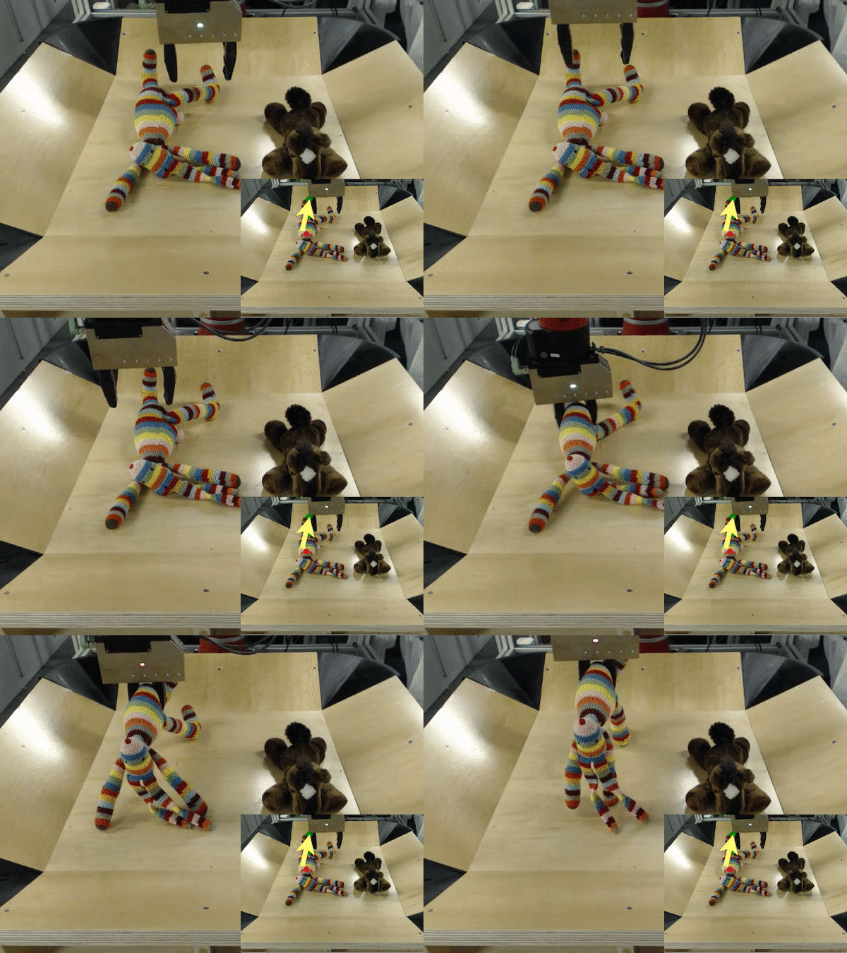
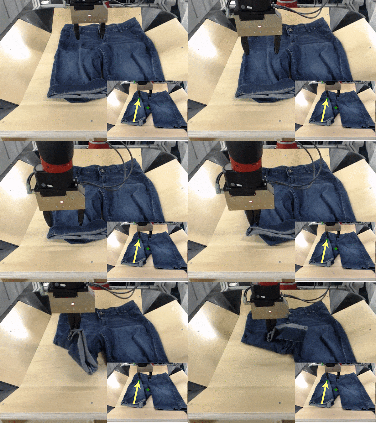
We have developed an algorithm that can learn a general-purpose predictive model
using unlabeled sensory experiences, and then use this single model to perform a
wide range of tasks.


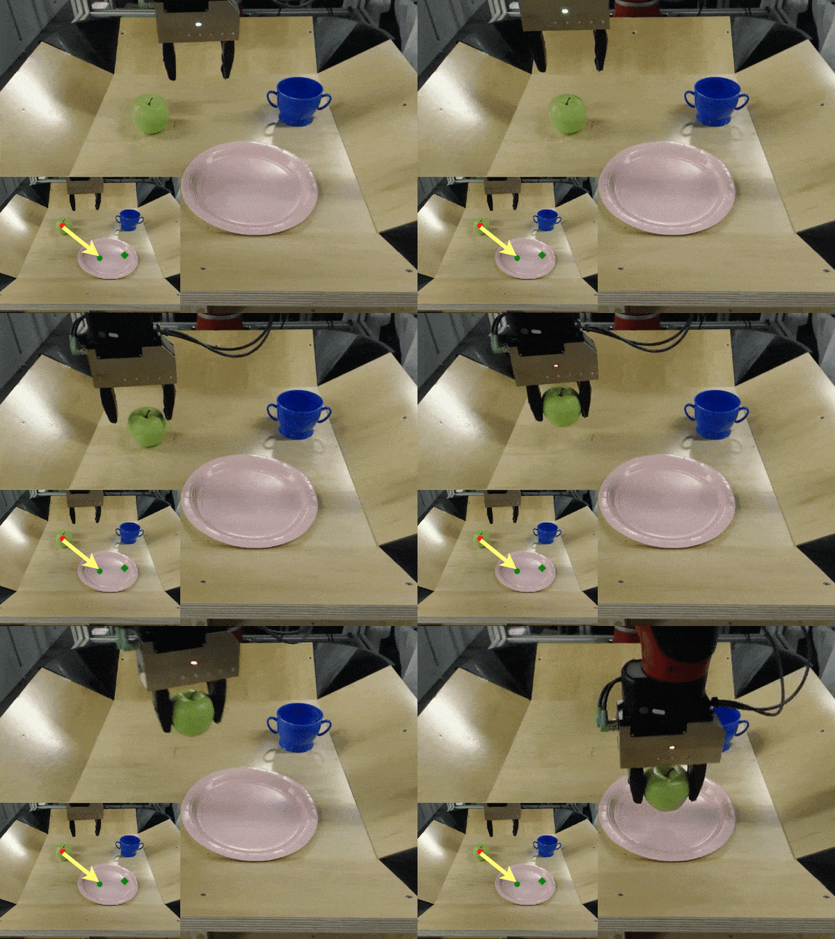
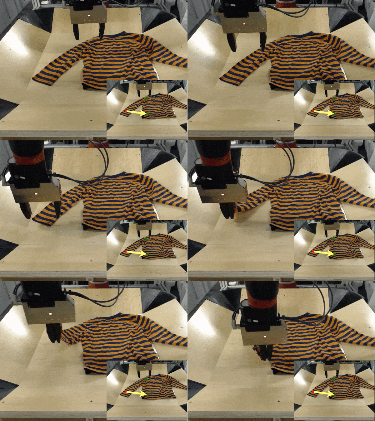
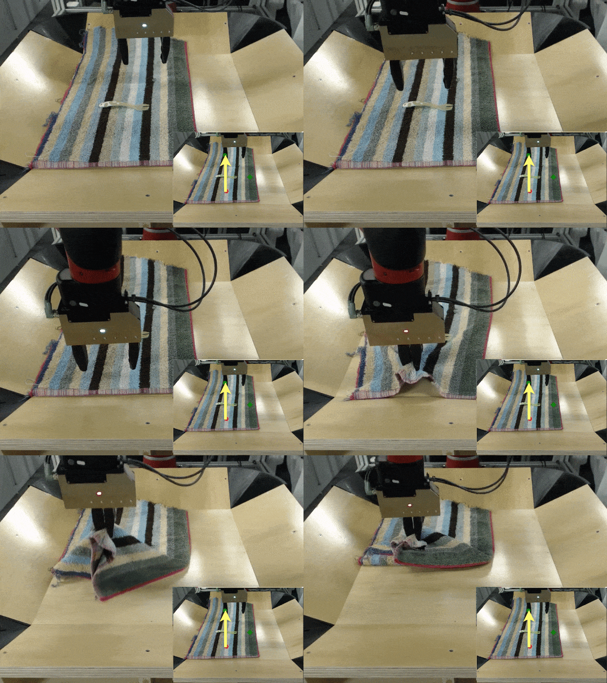
With a single model, our approach can perform a wide range of tasks, including
lifting objects, folding shorts, placing an apple onto a plate, rearranging
objects, and covering a fork with a towel.

In this post, we will describe how this works. We will discuss how we can learn
based on only raw sensory interaction data (i.e. image pixels, without requiring
object detectors or hand-engineered perception components). We will show how we
can use what was learned to accomplish many different user-specified tasks. And,
we will demonstrate how this approach can control a real robot from raw pixels,
performing tasks and interacting with objects that the robot has never seen
before.

Continue reading

Amazon SageMaker now comes with new capabilities for accelerating machine learning experimentation

Data scientists and developers can now quickly and easily organize, track, and evaluate their machine learning (ML) model training experiments on Amazon SageMaker. We are introducing a new Amazon SageMaker Search capability that lets you find and evaluate the most relevant model training runs from the hundreds and thousands of your Amazon SageMaker model training jobs. This accelerates the model development and experimentation phase, improves the productivity of data scientists and developers, and reduces overall time to market of machine-learning-based solutions. The new search capability is available in beta through both the AWS Management Console and the AWS SDK APIs for Amazon SageMaker. It’s available in 13 AWS Regions where Amazon SageMaker is currently available, at no additional charge to you.

Developing a machine learning model requires continuous experimentation and observation. For example, when you try a new learning algorithm or tune the model hyperparameters, you need to observe the impact of such incremental changes on model performance and accuracy. This iterative optimization exercise often leads to data explosion, with hundreds of model training experiments and model versions. This can slow down the convergence and discovery of the “winning” model. The information explosion also makes it cumbersome to trace back the antecedents of a model version deployed in a production environment. This difficulty in tracing model lineage hinders model auditing and compliance verifications, debugging a degradation in model’s live prediction performance and setting up new model retraining experiments.

Amazon SageMaker Search lets you quickly identify the most relevant model training runs for addressing your business use case. You can search on all of the defining attributes: the learning algorithm employed, hyperparameter settings, training datasets used, even the tags you have added on the model training jobs. Searching on tags lets you quickly find the model training runs associated with a specific business project, a research lab, or a data science team. This can help you meaningfully categorize and catalog your model training runs. In addition to tracking and organizing the relevant model training runs in a centralized place, you can quickly compare and rank them based on their performance metrics such as training loss and validation accuracy, thus creating leaderboards for picking “winning” models to deploy into production environments. Finally, with Amazon SageMaker search you can quickly trace back the lineage of a model deployed in live environments right to the data set used in training or validating the model. With a single click on the AWS Management Console or through simple one-line API calls, you can now access the specific training run along with all of the ingredients that went into creating the model in first place.

Now let’s dive into a step-by-step experience that shows you how you can efficiently manage your model training experiments using Amazon SageMaker Search. This new feature is available in beta, so use it with caution in production.

Organize, track, and evaluate model training experiments using Amazon SageMaker Search

In this example we’ll train a simple binary classification model on the MNIST data set using the Amazon SageMaker Linear Learner algorithm. The model will predict whether a given image is of the digit 0 or otherwise. We’ll experiment with tuning the hyperparameters of the Linear Learner algorithm, such as mini_batch_size, while optimizing for the binary_classification_accuracy metric that measures the accuracy of predictions made by the model. You can find the sample notebook for this example here.

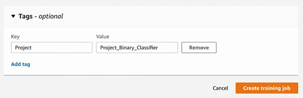
Step 1: Set up the experiment tracking by choosing a unique label for tagging all of the model training runs

You can add the tag while creating a model training job. Open the AWS Management Console and navigate to the Amazon SageMaker console.

You can also add the tag using the Amazon SageMaker Python SDK API while you are creating a training job using SageMaker estimator.

linear_1 = sagemaker.estimator.Estimator(
  linear_learner_container, role, 
  train_instance_count=1, train_instance_type = 'ml.c4.xlarge',
  output_path=<you model output S3 path URI>,
  tags=[{"Key":"Project", "Value":"Project_Binary_Classifier"}],
  sagemaker_session=sess)

Step 2: Perform multiple model training runs trying new hyperparameter settings each time

For demonstration purposes, we’ll try three different batch_sizes of 100, 200, and 300. Here is some sample code:

linear_1.set_hyperparameters(feature_dim=784,predictor_type='binary_classifier', mini_batch_size=100)
linear_1.fit({'train': <your training dataset S3 URI>})

We are consistently tagging all three model training runs with the same unique label so we can group them together under the same project. In the next step we’ll show you how you can use Amazon SageMaker Search to query and organize all of the model training runs labelled with our “Project” tag.

Step 3: Search and organize the relevant experiments at a centralized place for further evaluation

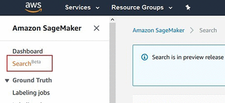
Search is available in beta on the Amazon SageMaker console.

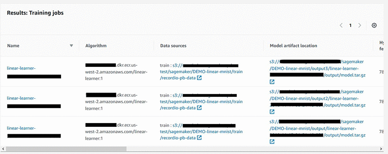
You can search all three model training runs that we performed in Step 2, by searching for the tag.

This lists all of the labelled training runs in a table.

You can also search using the AWS SDK API for Amazon SageMaker Search.

………………
search_params={
   "MaxResults": 10,
   "Resource": "TrainingJob",
   "SearchExpression": { 
      "Filters": [{ 
            "Name": "Tags.Project",
            "Operator": "Equals",
            "Value": "Project_Binary_Classifier"
         }]},
  "SortBy": "Metrics.train:binary_classification_accuracy",
  "SortOrder": "Descending"
}
smclient = boto3.client(service_name='sagemaker')
results = smclient.search(**search_params)

While we have demonstrated searching by tags, the new Amazon SageMaker Search supports searching on any metadata for model training runs, such as the learning algorithm used, training dataset URIs, and ranges of numerical values for hyperparameters and model training metrics.

Step 4: Sort on the objective performance metric of your choice to find the winning model

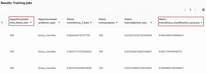
The model training jobs returned by Amazon SageMaker Search in Step 3 are presented to you in a table—like a leaderboard—with all of the hyperparameters and model training metrics presented in sortable columns. Choose the column header to rank the leaderboard for the objective performance metric of your choice, in this case, binary_classification_accuracy.

You can also print the leaderboard inline in your Amazon SageMaker Jupyter notebooks. Here is some sample code:

import pandas
headers=["Training Job Name", "Training Job Status", "Batch Size", "Binary Classification Accuracy"]
rows=[]
for result in results['Results']: 
    trainingJob = result['TrainingJob']
    metrics = trainingJob['FinalMetricDataList']
    rows.append([trainingJob['TrainingJobName'],
     trainingJob['TrainingJobStatus'],
     trainingJob['HyperParameters']['mini_batch_size'],
     metrics[[x['MetricName'] for x in  
     metrics].index('train:binary_classification_accuracy')]['Value']
    ])
df = pandas.DataFrame(data=rows,columns=headers)
from IPython.display import display, HTML
display(HTML(df.to_html()))

As you can see in Step 3, we had already given the sort criteria in the search() API call as “SortBy“:  “Metrics.train:binary_classification_accuracy” and “SortOrder“: “Descending” for returning the results sorted on metric of our interest. The previous sample code  parses the JSON response and presents the results in a leaderboard format, that looks like the following:

Now that you have identified the winning model—with batch_size = 300, and the highest classification accuracy of 0.99344—you can now deploy this model to a live endpoint. The sample notebook has step-by-step instructions for deploying an Amazon SageMaker endpoint.

Tracing a model’s lineage on Amazon SageMaker

Now we’ll show you an example of picking a prediction endpoint and quickly tracing back to the model training run used in creating the model deployed at the endpoint.

Using single-click on the Amazon SageMaker console

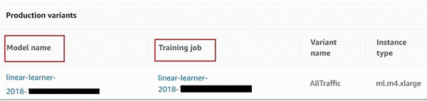
In the left navigation pane of the Amazon SageMaker, choose Endpoints, and select the relevant endpoint from the list of all your deployed endpoints. Scroll to Endpoint Configuration Settings, which lists all the model versions deployed at the endpoint. You will see an additional hyperlink to the Model Training Job that created that model in the first place.

Using the AWS SDK for Amazon SageMaker Search

You can also use few simple one-line API calls to quickly trace the lineage of a model.

#first get the endpoint config for the relevant endpoint
endpoint_config = smclient.describe_endpoint_config(EndpointConfigName=endpointName)

#now get the model name for the model deployed at the endpoint. 
model_name = endpoint_config['ProductionVariants'][0]['ModelName']

#now look up the S3 URI of the model artifacts
model = smclient.describe_model(ModelName=model_name)
modelURI = model['PrimaryContainer']['ModelDataUrl']

#search for the training job that created the model artifacts at above S3 URI location
search_params={
   "MaxResults": 1,
   "Resource": "TrainingJob",
   "SearchExpression": { 
      "Filters": [ 
         { 
            "Name": "ModelArtifacts.S3ModelArtifacts",
            "Operator": "Equals",
            "Value": modelURI
         }]}
}
results = smclient.search(**search_params)

Get started with more examples and developer support

Now that you have seen examples of how to efficiently manage the machine learning experimentation process and trace a model’s lineage using the new Amazon SageMaker Search, you can try out our sample notebook. You can also refer to our developer guide for more examples or post your questions on our developer forum. Happy experimenting!


About the Author

Sumit Thakur is a Senior Product Manager for AWS Machine Learning Platforms where he loves working on products that make it easy for customers to get started with machine learning on cloud. He is product manager for Amazon SageMaker and AWS Deep Learning AMI. In his spare time, he likes connecting with nature and watching sci-fi TV series.