
Blog

Learn About Our Meetup

5000+ Members

MEETUPS

LEARN, CONNECT, SHARE

Join our meetup, learn, connect, share, and get to know your Toronto AI community. 

JOB POSTINGS

INDEED POSTINGS

Browse through the latest deep learning, ai, machine learning postings from Indeed for the GTA.

CONTACT

CONNECT WITH US

Are you looking to sponsor space, be a speaker, or volunteer, feel free to give us a shout.

Category: Global

EfficientNet-EdgeTPU: Creating Accelerator-Optimized Neural Networks with AutoML

For several decades, computer processors have doubled their performance every couple of years by reducing the size of the transistors inside each chip, as described by Moore’s Law. As reducing transistor size becomes more and more difficult, there is a renewed focus in the industry on developing domain-specific architectures — such as hardware accelerators — to continue advancing computational power. This is especially true for machine learning, where efforts are aimed at building specialized architectures for neural network (NN) acceleration. Ironically, while there has been a steady proliferation of these architectures in data centers and on edge computing platforms, the NNs that run on them are rarely customized to take advantage of the underlying hardware.

Today, we are happy to announce the release of EfficientNet-EdgeTPU, a family of image classification models derived from EfficientNets, but customized to run optimally on Google’s Edge TPU, a power-efficient hardware accelerator available to developers through the Coral Dev Board and a USB Accelerator. Through such model customizations, the Edge TPU is able to provide real-time image classification performance while simultaneously achieving accuracies typically seen only when running much larger, compute-heavy models in data centers.

Using AutoML to customize EfficientNets for Edge TPU
EfficientNets have been shown to achieve state-of-the-art accuracy in image classification tasks while significantly reducing the model size and computational complexity. To build EfficientNets designed to leverage the Edge TPU’s accelerator architecture, we invoked the AutoML MNAS framework and augmented the original EfficientNet’s neural network architecture search space with building blocks that execute efficiently on the Edge TPU (discussed below). We also built and integrated a “latency predictor” module that provides an estimate of the model latency when executing on the Edge TPU, by running the models on a cycle-accurate architectural simulator. The AutoML MNAS controller implements a reinforcement learning algorithm to search this space while attempting to maximize the reward, which is a joint function of the predicted latency and model accuracy. From past experience, we know that Edge TPU’s power efficiency and performance tend to be maximized when the model fits within its on-chip memory. Hence we also modified the reward function to generate a higher reward for models that satisfy this constraint.

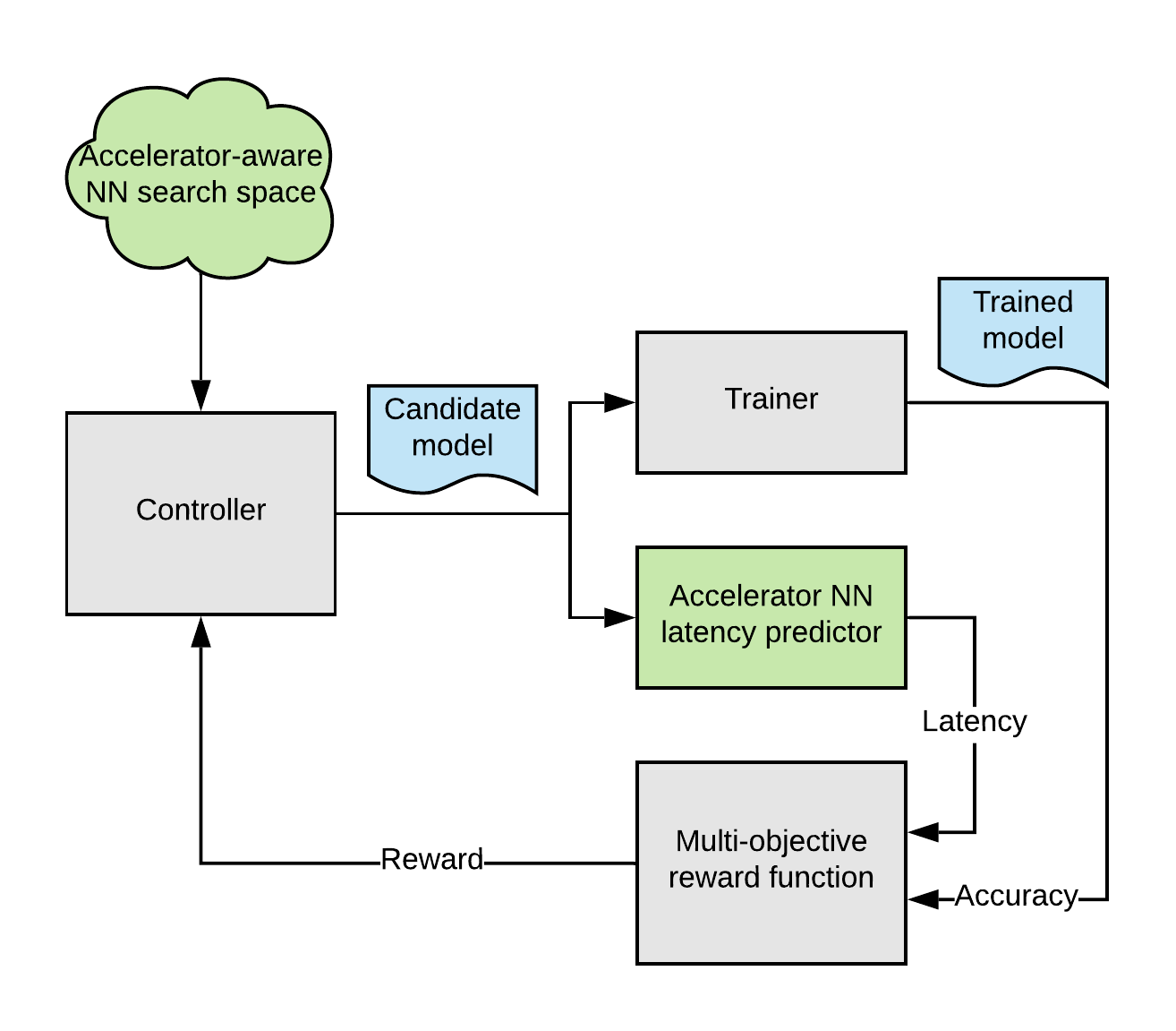
Overall AutoML flow for designing customized EfficientNet-EdgeTPU models.

Search Space Design
When performing the architecture search described above, one must consider that EfficientNets rely primarily on depthwise-separable convolutions, a type of neural network block that factorizes a regular convolution to reduce the number of parameters as well as the amount of computations. However, for certain configurations, a regular convolution utilizes the Edge TPU architecture more efficiently and executes faster, despite the much larger amount of compute. While it is possible, albeit tedious, to manually craft a network that uses an optimal combination of the different building blocks, augmenting the AutoML search space with these accelerator-optimal blocks is a more scalable approach.

A regular 3×3 convolution (right) has more compute (multiply-and-accumulate (mac) operations) than an depthwise-separable convolution (left), but for certain input/output shapes, executes faster on Edge TPU due to ~3x more effective hardware utilization.

In addition, removing certain operations from the search space that require modifications to the Edge TPU compiler to fully support, such swish non-linearity and squeeze-and-excitation block, naturally leads to models that are readily ported to the Edge TPU hardware. These operations tend to improve model quality slightly, so by eliminating them from the search space, we have effectively instructed AutoML to discover alternate network architectures that may compensate for any potential loss in quality.

Model Performance
The neural architecture search (NAS) described above produced a baseline model, EfficientNet-EdgeTPU-S, which is subsequently scaled up using EfficientNet’s compound scaling method to produce the -M and -L models. The compound scaling approach selects an optimal combination of input image resolution scaling, network width, and depth scaling to construct larger, more accurate models. The -M, and -L models achieve higher accuracy at the cost of increased latency as shown in the figure below.

EfficientNet-EdgeTPU-S/M/L models achieve better latency and accuracy than existing EfficientNets (B1), ResNet, and Inception by specializing the network architecture for Edge TPU hardware. In particular, our EfficientNet-EdgeTPU-S achieves higher accuracy, yet runs 10x faster than ResNet-50.

Interestingly, the NAS-generated model employs the regular convolution quite extensively in the initial part of the network where the depthwise-separable convolution tends to be less effective than the regular convolution when executed on the accelerator. This clearly highlights the fact that trade-offs usually made while optimizing models for general purpose CPUs (reducing the total number of operations, for example) are not necessarily optimal for hardware accelerators. Also, these models achieve high accuracy even without the use of esoteric operations. Comparing with the other image classification models such as Inception-resnet-v2 and Resnet50, EfficientNet-EdgeTPU models are not only more accurate, but also run faster on Edge TPUs.

This work represents a first experiment in building accelerator-optimized models using AutoML. The AutoML-based model customization can be extended to not only a wide range of hardware accelerators, but also to several different applications that rely on neural networks.

From Cloud TPU training to Edge TPU deployment
We have released the training code and pretrained models for EfficientNet-EdgeTPU on our github repository. We employ tensorflow’s post-training quantization tool to convert a floating-point trained model to an Edge TPU-compatible integer-quantized model. For these models, the post-training quantization works remarkably well and produces only a very slight loss in accuracy (~0.5%). The script for exporting the quantized model from a training checkpoint can be found here. For an update on the Coral platform, see this post on the Google Developer’s Blog, and for full reference materials and detailed instructions, please refer to the Coral website.

Acknowledgements
Special thanks to Quoc Le, Hongkun Yu, Yunlu Li, Ruoming Pang, and Vijay Vasudevan from the Google Brain team; Bo Wu, Vikram Tank, and Ajay Nair from the Google Coral team; Han Vanholder, Ravi Narayanaswami, John Joseph, Dong Hyuk Woo, Raksit Ashok, Jason Jong Kyu Park, Jack Liu, Mohammadali Ghodrat, Cao Gao, Berkin Akin, Liang-Yun Wang, Chirag Gandhi, and Dongdong Li from the Google Edge TPU team.

Use Amazon Lex as a conversational interface with Twilio Media Streams

Businesses use the Twilio platform to build new ways to communicate with their customers: whether it’s fully automating a restaurant’s food orders with a conversational Interactive Voice Response (IVR) or building a next generation advanced contact center. With the launch of Media Streams, Twilio is opening up their Voice platform by providing businesses access to the raw audio stream of their phone calls in real time.

You can use Media Streams to increase productivity in the call center by transcribing speech in real time with Amazon Transcribe Streaming WebSockets or to automate end-user interactions and make recommendations to agents based on the caller’s intent using Amazon Lex.

In this blog post, we show you how to use Amazon Lex to integrate conversational interfaces (chatbots) to your voice application using the raw audio stream provided by Twilio Media Streams. Lex uses deep learning to do the heavy lifting required to recognize the intent of human speech so that you can easily build engaging user experiences and lifelike conversations.

The solution follows these steps:

  1. Receive audio stream from Twilio
  2. Send the audio stream to a voice activity detection component to determine voice in audio
  3. Start streaming the user data to Amazon Lex when voice is detected
  4. Stop streaming the user data to Amazon Lex when silence is detected
  5. Update the ongoing Twilio call based on the response from Amazon Lex

The Voice activity detection (VAD) implementation provided in this sample is for reference/demo purpose only and uses a rudimentary approach to detect voice and silence by looking at amplitude. It is not recommended for production use. You will need to implement a robust form of VAD module as per your need for use in production scenarios.

The diagram below describes the steps:

The instructions for integrating an Amazon Lex Bot with the Twilio Voice Stream are provided in the following steps:

  • Step 1: Create an Amazon Lex Bot
  • Step 2: Create a Twilio Account and Setup Programmable Voice
  • Step 3: Build and Deploy the Amazon Lex and Twilio Voice Stream Integration code to Amazon ECS/Fargate
  • Step 4: Test the deployed service
  • As an optional next step, you can build and test the service locally. For instructions, see Step 5 (Optional): Build and Test the service locally

To build and deploy the service, the following pre-requisites are needed:

  1. Python (The language used to build the service)
  2. Docker (The tool used for packaging the service for deployment)
  3. AWS CLI installed and configured (For creating the required AWS services and deploying the service to AWS). For instructions see, Configuring AWS CLI

In addition, you need a domain name for hosting your service and you must register an SSL certificate for the domain using Amazon Certificate Manager.  For instructions, see Request a Public Certificate. Record the Certificate ARN from the console.

An SSL certificate is needed to communicate securely over wss (WebSocket Secure), a persistent bidirectional communication protocol used by the Twilio voice stream. The <Stream> instruction in the templates/streams.xml file allows you to receive raw audio streams from a live phone call over WebSockets in near real-time. On successful connection, a WebSocket connection to the service is established and audio will start streaming.

Step 1: Create an Amazon Lex Bot

If you don’t already have an Amazon Lex Bot, create and deploy one. For instructions, see Create an Amazon Lex Bot Using a Blueprint (Console).

Once you’ve created the bot, deploy the bot and create an alias. For instructions, see Publish a Version and Create an Alias.

In order to call the Amazon Lex APIs from the service, you must create an IAM user with an access type “Programmatic Access” and attach the appropriate policies.

For this, in the AWS Console, go to IAM->Users->Add user

Provide a user name, select “Programmatic access” Access type, then click on “Next: Permissions”

Using the “Attach existing policies directly” option, filter for Amazon Lex policies and select AmazonLexReadOnly and AmazonLexRunBotsOnly policies.

Click “Next: Tags”, “Next: Review”, and “Create User” in the pages that follow to create the user. Record the access key ID and the secret access key. We use these credentials during the deployment of the stack.

Step 2: Create a Twilio account and setup programmable voice

Sign up for a Twilio account and create a programmable voice project.

For sign-up instructions, see https://www.twilio.com/console.

Record the “AUTH TOKEN”. You can find this information on the Twilio dashboard under Settings->General->API Credentials.

You must also verify the caller ID by adding the phone number that you are using to make calls to the Twilio phone number. You can do this by clicking on the   button on the Verify caller IDs page.

Step 3: Build and deploy the Amazon Lex and Twilio Stream Integration code to Amazon ECS

In this section, we create a new service using AWS Fargate to host the integration code. AWS Fargate is a deployment option in Amazon Elastic Container Service (ECS) that allows you to deploy containers without worrying about provisioning or scaling servers. For our service, we use Python and Flask in a Docker container behind an Application Load Balancer (ALB).

Deploy the core infrastructure

As the first step in creating the infrastructure, we deploy the core infrastructure components such as VPC, Subnets, Security Groups, ALB, ECS cluster, and IAM policies using a CloudFormation Template.

Clicking on the “Launch Stack” button below takes you to the AWS CloudFormation Stack creation page. Click “Next” and fill in the parameters. Please note that you will be using the same “EnvironmentName” parameter later in the process where we will be launching the service on top of the core infrastructure. This allows us to reference the stack outputs from this deployment.

Once the stack creation is complete, from the “outputs” tab, record the value of the “ExternalUrl” key.

Package and deploy the code to AWS

In order to deploy the code to Amazon ECS, we package the code in a Docker container and upload the Docker image to the Amazon Elastic Container Registry (ECR).

The code for the service is available at the GitHub repository below. Clone the repository on your local machine.

git clone https://github.com/veerathp/lex-twiliovoice.git
cd lex-twiliovoice

Next, we update the URL for the Streams element inside templates/streams.xml to match the DNS name for your service that you configured with the SSL certificate in the pre-requisites section.

<Stream url="wss://<Your DNS>/"></Stream>

Now, run the following command to build the container image using the Dockerfile.

docker build -t lex-twiliovoice .

Next, we create the container registry using the AWS CLI by passing in the value for the repository name. Record the “repositoryUri” from the output.

aws ecr create-repository --repository-name <repository name>

In order to push the container image to the registry, we must authenticate. Run the following command:

aws ecr get-login --region us-west-2 --no-include-email

Execute the output of the above command to complete the authentication process.

Next, we tag and push the container image to ECR.

docker tag lex-twiliovoice <repositoryUri>/lex-twiliovoice:latest
docker push <repositoryUri>/lex-twiliovoice:latest

We now deploy the rest of the infrastructure using a CloudFormation template. As part of this stack, we deploy components such as ECS Service, ALB Target groups, HTTP/HTTPS Listener rules, and Fargate Task. The environment variables are injected into the container using the task definition properties.

Since we are working with WebSocket connections in our service, we enable stickiness with our load balancer using the target group attribute to allow for persistent connection with the same instance.

TargetGroup:
    Type: AWS::ElasticLoadBalancingV2::TargetGroup
    Properties:
      ….
      ….
      TargetGroupAttributes:
        - Key: stickiness.enabled
          Value: true
        …

Clicking on the “Launch Stack” button below takes you to the AWS CloudFormation Stack creation page. Click “Next” and fill in the correct values for the following parameters that are collected from the previous steps – IAMAccessKeyId, IAMSecretAccessKey, ImageUrl, LexBotName, LexBotAlias, and TwilioAuthToken. You can use default values for all the other parameters. Make sure to use the same “EnvironmentName” from the previous stack deployment since we are referring to the outputs of that deployment.

Once the deployment is complete, we can test the service. However, before we do that, make sure to point your custom DNS to the Application Load Balancer URL.

To do that, we create an “A Record” under Route 53, Hosted Zones to point your custom DNS to the ALB Url that was part of the core infrastructure stack deployment (“ExternalUrl” key from output). In the “Create Record Set” screen, in the name field use your DNS name, for type select “A – IPv4 address”, select “Yes” for Alias field, select the Alias target as the ALB Url, and click “Create”.

Step 4: Test the deployed service

You can verify the deployment by navigating to the Amazon ECS Console and clicking on the cluster name. You can see the AWS Fargate service under the “services” tab and the running task under the “tasks” tab.

To test the service, we will first update the Webhook url field under the “Voice & Fax” section in the Twilio console with the URL of the service that is running in AWS (http://<url>/twiml). You can now call the Twilio phone number to reach the Lex Bot. Make sure that the number you are calling from is verified using the Twilio console. Once connected, you will hear the prompt “You will be interacting with Lex bot in 3, 2, 1. Go.” that is configured in the templates/streams.xml file. You can now interact with the Amazon Lex Bot.

You can monitor the service using the “CloudWatch Log Groups” and troubleshoot any issues that may arise while the service is running.

Step 5(Optional): Build and test the service locally

Now that the service is deployed and tested, you may be interested in building and testing the code locally. For this, navigate to the cloned GitHub repository on your local machine and install all the dependencies using the following command:

pip install -r requirements.txt

You can test the service locally by installing “ngrok”. See https://ngrok.com/download for more details. This tool provides public URLs for exposing the local web server. Using this, you can test the Twilio webhook integration.

Start the ngrok process by using the following command in another terminal window. The ngrok.io url can be used to access the web service from external applications.

ngrok http 8080

Next, configure the “Stream” element inside the templates/streams.xml file with the correct ngrok url.

<Stream url="wss://<xxxxxxxx.ngrok.io>/"></Stream>

In addition, we also need to configure the environment variables used in the code. Run the following command after providing appropriate values for the environment variables:

export AWS_REGION=us-west-2
export ACCESS_KEY_ID=<Your IAM User Access key ID from Step 1>
export SECRET_ACCESS_KEY=<Your IAM User Secret Access key from Step 1>
export LEX_BOT_NAME=<Bot name for the Lex Bot you created in Step 1>
export LEX_BOT_ALIAS=<Bot Alias for the Lex Bot you created in Step 1>
export TWILIO_AUTH_TOKEN=<Twilio AUTH TOKEN from Step 2>
export CONTAINER_PORT=8080
export URL=<http://xxxxxxxx.ngrok.io> (update with the appropriate url from ngrok)

Once the variables are set, you can start the service using the following command:

python server.py

To test, configure the Webhook field under “Voice & Fax” in the Twilio console with the correct url (http://<url>/twiml) as shown below.

Initiate a call to the Twilio phone number from a verified phone. Once connected, you hear the prompt “You will be interacting with Lex bot in 3, 2, 1. Go.” that is configured in the templates/streams.xml file. You are now able to interact with the Amazon Lex bot that you created in Step 1.

In this blog post, we showed you how to use Amazon Lex to integrate your chatbot to your voice application. To learn how to build more with Amazon Lex, check out the developer resources.


About the Author

Praveen Veerath is a Senior AI Solutions Architect for AWS.


Ultrasounds Where You Need Them: How AI Is Improving Diagnoses at Point of Care

In medical emergencies, a quick diagnosis based on the information at hand can be a matter of life or death.

The same can be true for non-emergencies. When limited medical equipment is available, delays in diagnosis can turn these situations into emergencies.

Ultrasound enables the accurate, efficient and non-invasive diagnosis of a host of ailments, including appendicitis, heart abnormalities and many urological and gynecological conditions.

But most emergency responders and medical professionals either aren’t trained or aren’t equipped to use the technology.

DESKi, a member of the NVIDIA Inception program, based in Bordeaux, France, is using AI to make ultrasound technologies more effective at the point of care for these personnel and their patients.

“The fact that two-thirds of the world population have no access to medical imaging technologies is a public health issue,” said Bertrand Moal, CEO at DESKi. “Ultrasound is non-invasive, affordable and can be used to diagnose ailments of multiple organs, which makes it the perfect tool to support diagnosis at the point of care, by non-specialists.”

Benefits of Ultrasound

To help those on the medical front lines make more accurate diagnoses and better informed decisions about patient care, DESKi has created DeepEcho.

This system combines deep learning algorithms, trained on NVIDIA DGX Station, and cutting-edge handheld ultrasound devices, which can be linked up to mobile phones and tablets, to deliver the expertise of cardiac health specialists in emergency situations.

Using a wealth of training data from leading cardiology units, DESKi has developed a series of neural networks that can determine whether or not the DeepEcho’s ultrasound probe is in the correct position for acquiring accurate and insightful views of the heart.

The company is also training its algorithms to automatically measure the left ventricle ejection fraction, which can help diagnose heart failure.

“By deploying ultrasound in the field with AI software, we’re helping to bring medical imaging expertise to those who need it most,” said Moal.


Protecting Patient Privacy

To train their deep learning algorithms, DESKi needs to collect high-quality data that has been reviewed and interpreted by cardiology experts.

Recently, the startup entered into a framework agreement with Bordeaux University Hospital for the development of AI projects, including DeepEcho.

Over 20,000 cardiac ultrasound examinations are performed by experienced cardiologists every year at the hospital. DESKi uses anonymized data from these examinations to train its deep learning algorithms.

To accelerate the training, DESKi turned to the power of NVIDIA DGX Station. The portability of the deskside supercomputer enabled them to build the initial framework in-house; when it was time to deploy, they transported the system to the hospital itself.

“By deploying NVIDIA’s DGX Station onsite in the hospital, we’re able to combine cutting-edge AI technology with cardiology expertise, all while ensuring that patient data is secure and never comes off premises,” noted Victor Ferrand, co-founder and CTO at DESKi.

In the future, DESKi plans to expand its tools to other specialties such as gynecology, gastroenterology and urology.

Learn more about their work with Bordeaux University Hospital in our webinar “Deep Learning for Automatic Cardiac Ultrasound Analysis.”

The post Ultrasounds Where You Need Them: How AI Is Improving Diagnoses at Point of Care appeared first on The Official NVIDIA Blog.

Harvesting success using Amazon SageMaker to power Bayer’s digital farming unit

By the year 2050, our planet will need to feed ten billion people. We can’t expand the earth to create more agricultural land, so the solution to growing more food is to make agriculture more productive and less resource-dependent. In other words, there is no room for crop losses or resource waste. Bayer is using Amazon SageMaker to help eliminate losses from happening in fields around the world.

Households contribute to food loss by discarding food such as kitchen waste or leftover cooked meals. However, the vast majority of food loss in many countries is actually from crops that “die on the vine” in one form or another—from pests, diseases, weeds, or poor nutrition in the soil. The Climate Corporation—a Bayer subsidiary—provides digital farming offerings that help resolve these challenges.

The Climate Corporation’s solutions include automatic recording of data from tractors and satellite-enabled field-health maps. By delivering these services and others to thousands of farmers globally, The Climate Corporation enables farmers to keep their land healthy and fertile.

The team is also working on an upcoming service called FieldCatcher that enables farmers to use smartphone images to identify weeds, pests, and diseases. “By using image recognition, we provide farmers with access to a virtual agronomist that helps with the often difficult task to identify the cause of crop issues. This empowers farmers who don’t have access to advice, as well as enable all farmers to more efficiently capture and share field observations,” said Matthias Tempel, Proximal Sensing Lead at The Climate Corporation.

FieldCatcher uses image recognition models trained with Amazon SageMaker, then optimizes them for mobile phones with Amazon SageMaker Neo. With this setup, the farmers are able to use the model and get instant results even without internet access (as many fields lack connectivity). Using Amazon SageMaker helps FieldCatcher to identify the cause of the problem with confidence, which is critical to providing farmers with the right remediation guidance. In many cases, acting immediately and being certain about an issue makes a huge difference for fields’ yields and farmers’ success.

To power the FieldCatcher solution, Bayer collects images—seeking a wide variety as well as a high quantity to create training data that includes various environments, growth stages, weather conditions, and levels of daylight. Each photo is uploaded from a smartphone and eventually becomes part of the ongoing library that makes the recognition better and better. The figure below depicts the journey of each image and its metadata.

Specifically, the process starts with ingestion to Amazon Cognito, which protects uploads to the Amazon API Gateway and Amazon Simple Storage Service (Amazon S3). The serverless architecture—chosen because it is more scalable and easier to maintain than any alternative—relies on AWS Lambda to execute its steps and finally move the received data into a data lake.

Multiple AWS services work in concert to support the data lake. In addition to Amazon S3 for image storing, Amazon DynamoDB stores the metadata, as features of the image such as location and date taken are important for searchability later on. Amazon Elasticsearch Service (Amazon ES) powers the indexing and querying of this metadata.

The engineering team appreciates that this set of services does not require a data schema to be defined upfront, enabling many different possible use cases for images to be collected in the FieldCatcher application. Another benefit is that the data lake queries allow questions as different as “search for all images taken in Germany with an image resolution larger than 800×600 pixels” or “search for all images of diseases in winter wheat.”

For machine learning (ML) model development, training, and inferencing, the team relies on Amazon SageMaker. Specifically, Amazon SageMaker’s built-in Jupyter notebooks are the central workspace for developing ML models as well as the corresponding ML algorithms. Developers also use GitLab for source code management and GitLab-CI for automated tasks.

AWS Step Functions are the final piece, used to support the full roundtrip of preprocessing images from the data lake, automated training of ML models, and finally inference. Using these services, Bayer’s developers can operate with confidence in the infrastructure and can focus on the ML models.

The Bayer team members, as longstanding AWS users, are familiar with the power of ML to solve problems that would otherwise be exceedingly complex for humans to tackle. The company previously developed an AWS based data-collection and analysis platform that leverages AWS IoT and sensors in the harvest fields to power real-time decision-making with information fed to mobile devices.

Their choice to expand their offerings to include the new FieldCatcher application was driven by the positive feedback from some of these other services. Giuseppe La Tona, Enterprise Solution Architect at The Climate Corporation described, “We used to make this type of service fully ourselves, but it was an enormous amount of work to do and maintain. We realized that, with Amazon SageMaker, the solution was infinitely easier, so we started implementing it and have never looked back.”

At the moment, FieldCatcher is used internally in over 20 countries around the world. The next step is expanding what it can offer farmers. Right now, its main use is for weed, disease, or pest detection. The Climate Corporation is exploring additional ML-powered solutions as broad as predicting harvest quality with images and drone-based crop protection on an individual plant level. 

Going forward, the team plans to use Amazon SageMaker for all their ML work, as it has been so powerful and saved them so much time. In fact, the team’s entire workflow uses only AWS for ML. Alexander Roth Cloud Architect at Bayer, explained, “With machine learning on AWS, the huge impact we’ve seen is that the whole pipeline runs smoothly and we’re able to reduce errors.”

With these solutions in place and constantly improving (as is inherent to ML), Bayer and The Climate Corporation see themselves as pioneering the sustainable agriculture of the future. Their hope is that this effort and others it inspires will make it possible to support our growing population for years to come.


About the Author

Marisa Messina is on the AWS ML marketing team, where her job includes identifying the most innovative AWS-using customers and showcasing their inspiring stories. Prior to AWS, she worked on consumer-facing hardware and then university-facing cloud offerings at Microsoft. Outside of work, she enjoys exploring the Pacific Northwest hiking trails, cooking without recipes, and dancing in the rain.


An Interactive, Automated 3D Reconstruction of a Fly Brain

The goal of connectomics research is to map the brain’s “wiring diagram” in order to understand how the nervous system works. A primary target of recent work is the brain of the fruit fly (Drosophila melanogaster), which is a well-established research animal in biology. Eight Nobel Prizes have been awarded for fruit fly research that has led to advances in molecular biology, genetics, and neuroscience. An important advantage of flies is their size: Drosophila brains are relatively small (one hundred thousand neurons) compared to, for example, a mouse brain (one hundred million neurons) or a human brain (one hundred billion neurons). This makes fly brains easier to study as a complete circuit.

Today, in collaboration with the Howard Hughes Medical Institute (HHMI) Janelia Research Campus and Cambridge University, we are excited to publish “Automated Reconstruction of a Serial-Section EM Drosophila Brain with Flood-Filling Networks and Local Realignment”, a new research paper that presents the automated reconstruction of an entire fruit fly brain. We are also making the full results available for anyone to download or to browse online using an interactive, 3D interface we developed called Neuroglancer.

A 40-trillion pixel fly brain reconstruction, open to anyone for interactive viewing. Bottom right: smaller datasets that Google AI analyzed in publications in 2016 and 2018.

Automated Reconstruction of 40 Trillion Pixels
Our collaborators at HHMI sectioned a fly brain into thousands of ultra-thin 40-nanometer slices, imaged each slice using a transmission electron microscope (resulting in over forty trillion pixels of brain imagery), and then aligned the 2D images into a coherent, 3D image volume of the entire fly brain. Using thousands of Cloud TPUs we then applied Flood-Filling Networks (FFNs), which automatically traced each individual neuron in the fly brain.

While the algorithm generally performed well, we found performance degraded when the alignment was imperfect (image content in consecutive sections was not stable) or when occasionally there were multiple consecutive slices missing due to difficulties associated with the sectioning and imaging process. In order to compensate for these issues we combined FFNs with two new procedures. First, we estimated the slice-to-slice consistency everywhere in the 3D image and then locally stabilized the image content as the FFN traced each neuron. Second, we used a “Segmentation-Enhanced CycleGAN” (SECGAN) to computationally “hallucinate” missing slices in the image volume. SECGANs are a type of generative adversarial network specialized for image segmentation. We found that the FFN was able to trace through locations with multiple missing slices much more robustly when using the SECGAN-hallucinated image data.

Interactive Visualization of the Fly Brain with Neuroglancer
When working with 3D images that contain trillions of pixels and objects with complicated shapes, visualization is both essential and difficult. Inspired by Google’s history of developing new visualization technologies, we designed a new tool that was scalable and powerful, but also accessible to anybody with a web browser that supports WebGL. The result is Neuroglancer, an open-source project (github) that enables viewing of petabyte-scale 3D volumes, and supports many advanced features such as arbitrary-axis cross-sectional reslicing, multi-resolution meshes, and the powerful ability to develop custom analysis workflows via integration with Python. This tool has become heavily used by collaborators at the Allen Institute for Brain Science, Harvard University, HHMI, Max Planck Institute, MIT, Princeton University, and elsewhere.

A recorded demonstration of Neuroglancer. Interactive version available here.

Next Steps
Our collaborators at HHMI and Cambridge University have already begun using this reconstruction to accelerate their studies of learning, memory, and perception in the fly brain. However, the results described above are not yet a true connectome since establishing a connectome requires the identification of synapses. We are working closely with the FlyEM team at Janelia Research Campus to create a highly verified and exhaustive connectome of the fly brain using images acquired with “FIB-SEM” technology.

Acknowledgements
We would like to acknowledge core contributions from Tim Blakely, Viren Jain, Michal Januszewski, Laramie Leavitt, Larry Lindsey, Mike Tyka (Google), as well as Alex Bates, Davi Bock, Greg Jefferis, Feng Li, Mathew Nichols, Eric Perlman, Istvan Taisz, and Zhihao Zheng (Cambridge University, HHMI Janelia, Johns Hopkins University, and University of Vermont).

Git integration now available for the Amazon SageMaker Python SDK

Git integration is now available in the Amazon SageMaker Python SDK. You no longer have to download scripts from a Git repository for training jobs and hosting models. With this new feature, you can use training scripts stored in Git repos directly when training a model in the Python SDK. You can also use hosting scripts stored in Git repos when hosting a model. The scripts are hosted in GitHub, another Git-based repo, or an AWS CodeCommit repo.

This post describes in detail how to use Git integration with the Amazon SageMaker Python SDK.

Overview

When you train a model with the Amazon SageMaker Python SDK, you need a training script that does the following:

  • Loads data from the input channels
  • Configures training with hyperparameters
  • Trains a model
  • Saves the model

You specify the script as the value of the entry_point argument when you create an estimator object.

Previously, when users constructed an Estimator or Model object, in the Python SDK, the training script had to be a path in the local file system when you provided it as the entry_point value. This location was inconvenient when you had training scripts in Git repos because you had to download them locally.

If multiple developers were contributing to the Git repo, you would have to keep track of any updates to the repo. Also, if your local version was out of date, you’d need to pull the latest version prior to every training job. This also makes scheduling periodic training jobs even more challenging.

With the launch of Git integration, these issues are solved, which results in a notable improvement in convenience and productivity.

Walkthrough

Enable the Git integration feature by passing a dict parameter named git_config when you create the Estimator or Model object. The git_config parameter provides information about the location of the Git repo that contains the scripts and the authentication for accessing that repo.

Locate the Git repo

To locate the repo that contains the scripts, use the repo, branch, and commit fields in git_config. The repo field is required; the other two fields are optional. If you only provide the repo field, the latest commit in master branch is used by default:

git_config = {'repo': 'your-git-repo-url'}

To specify a branch, use both the repo and branch fields. The latest commit in that branch is used by default:

git_config = {'repo': 'your-git-repo-url', 'branch': 'your-branch'}

To specify a commit of a specific branch in a repo, use all three fields in git_config:

git_config = {'repo': 'your-git-repo-url', 
              'branch': 'your-branch', 
              'commit': 'a-commit-sha-under-this-branch'}

If only the repo and commit fields are provided, this works when the commit is under the master branch and the commit is used. However, if the commit is not under the master branch, the repo is not found:

git_config = {'repo': 'your-git-repo-url', 'commit': 'a-commit-sha-under-master'}

Get access to the Git repo

If the Git repo is private (all CodeCommit repos are private), you need authentication information to access it.

For CodeCommit repos, first make sure that you set up your authentication method. For more information, see Setting Up for AWS CodeCommit. The topic lists the following ways by which you can authenticate:

Authentication for SSH URLs

For SSH URLs, you must configure the SSH key pair. This applies to GitHub, CodeCommit, and other Git-based repos.

Do not set an SSH key passphrase for the SSH key pairs. If you do, access to the repo fails.

After the SSH key pair is configured, Git integration works with SSH URLs without further authentication information:

# for GitHub repos
git_config = {'repo': 'git@github.com:your-git-account/your-git-repo.git'}

# for CodeCommit repos
git_config = {'repo': 'ssh://git-codecommit.us-west-2.amazonaws.com/v1/repos/your-repo/'}

Authentication for HTTPS URLs

For HTTPS URLs, there are two ways to deal with authentication:

  • Have it configured locally.
  • Configure it by providing extra fields in git_config, namely 2FA_enabled, username, password, and token. Things can be slightly different here between CodeCommit, GitHub, and other Git-based repos.

Authenticating using Git credentials

If you authenticate with Git credentials, you can do one of the following:

  1. Provide the credentials in git_config:
    git_config = {'repo': 'https://git-codecommit.us-west-2.amazonaws.com/v1/repos/your-repo/',
                  'username': 'your-username',
                  'password': 'your-password'}

  2. Have the credentials stored in local credential storage. Typically, the credentials are stored automatically after you provide them with the AWS CLI. For example, macOS stores credentials in Keychain Access.

With the Git credentials stored locally, you can specify the git_config parameter without providing the credentials, to avoid showing them in scripts:

git_config = {'repo': 'https://git-codecommit.us-west-2.amazonaws.com/v1/repos/your-repo/'}

Authenticating using AWS CLI Credential Helper

If you follow the setup documentation mentioned earlier to configure AWS CLI Credential Helper, you don’t have to provide any authentication information.

For GitHub and other Git-based repos, check whether two-factor authentication (2FA) is enabled for your account. (Authentication is disabled by default and must be enabled manually.) For more information, see Securing your account with two-factor authentication (2FA).

If 2FA is enabled for your account, provide 2FA_enabled when specifying git_config and set it to True. Otherwise, set it to False. If 2FA_enabled is not provided, it is set to False by default. Usually, you can use either username+password or a personal access token to authenticate for GitHub and other Git-based repos. However, when 2FA is enabled, you can only use a personal access token.

To use username+password for authentication:

git_config = {'repo': 'https://github.com/your-account/your-private-repo.git',
              'username': 'your-username',
              'password': 'your-password'}

Again, you can store the credentials in local credential storage to avoid showing them in the script.

To use a personal access token for authentication:

git_config = {'repo': 'https://github.com/your-account/your-private-repo.git',
              'token': 'your-token'}

Create the estimator or model with Git integration

After you correctly specify git_config, pass it as a parameter when you create the estimator or model object to enable Git integration. Then, make sure that the entry_point, source_dir, and dependencies are all be relative paths under the Git repo.

You know that if source_dir is provided, entry_point should be a relative path from the source directory. The same is true with Git integration.


For example, with the following structure of the Git repo ‘amazon-sagemaker-examples’ under branch ‘training-scripts’:

amazon-sagemaker-examples 
   |
   |-------------char-rnn-tensorflow
   |                          |----------train.py
   |                          |----------utils.py
   |                          |----------other files
   |
   |-------------pytorch-rnn-scripts
   |-------------.gitignore
   |-------------README.md

You can create the estimator object as follows:

git_config = {'repo': 'https://github.com/awslabs/amazon-sagemaker-examples.git', 'branch': 'training-scripts'}

estimator = TensorFlow(entry_point='train.py',
                       source_dir='char-rnn-tensorflow',
                       git_config=git_config,
                       train_instance_type=train_instance_type,
                       train_instance_count=1,
                       role=sagemaker.get_execution_role(), # Passes to the container the AWS role that you are using on this notebook
                       framework_version='1.13',
                       py_version='py3',
                       script_mode=True)

In this example, source_dir 'char-rnn-tensorflow' is a relative path inside the Git repo, while entry_point 'train.py' is a relative path under ‘char-rnn-tensorflow’.

Git integration example

Now let’s look at a complete example of using Git integration. This example trains a multi-layer LSTM RNN model on a language modeling task based on PyTorch example. By default, the training script uses the Wikitext-2 dataset. We train a model on SageMaker, deploy it, and then use deployed model to generate new text.

Run the commands in a Python script, except for those that start with a ‘!’, which are bash commands.

First let’s do the setup:

import sagemaker
 sagemaker_session = sagemaker.Session()
 bucket = sagemaker_session.default_bucket()
 prefix = 'sagemaker/DEMO-pytorch-rnn-lstm'
 role = sagemaker.get_execution_role()

Next get the dataset. This data is from Wikipedia and is licensed CC-BY-SA-3.0. Before you use this data for any other purpose than this example, you should understand the data license, described at https://creativecommons.org/licenses/by-sa/3.0/:

!wget http://research.metamind.io.s3.amazonaws.com/wikitext/wikitext-2-raw-v1.zip
 !unzip -n wikitext-2-raw-v1.zip
 !cd wikitext-2-raw
 !mv wiki.test.raw test && mv wiki.train.raw train && mv wiki.valid.raw valid

Upload the data to S3:

inputs = sagemaker_session.upload_data(path='wikitext-2-raw', bucket=bucket, key_prefix=prefix)

Specify git_config and create the estimator with it:

from sagemaker.pytorch import PyTorch

git_config = {'repo': 'https://github.com/awslabs/amazon-sagemaker-examples.git', 'branch': 'training-scripts'}

estimator = PyTorch(entry_point='train.py',
                     role=role,
                     framework_version='1.1.0',
                     train_instance_count=1,
                     train_instance_type='ml.c4.xlarge',
                     source_dir='pytorch-rnn-scripts',
                     git_config=git_config,
                     hyperparameters={
                         'epochs': 6,
                         'tied': True
                     })

Train the mode:

estimator.fit({'training': inputs})

Next let’s host the model. We are going to provide custom implementation of model_fninput_fnoutput_fn, and predict_fn hosting functions in a separate file ‘generate.py’, which is in the same Git repo. The PyTorch model uses a npy serializer and deserializer by default. For this example, since we have a custom implementation of all the hosting functions and plan on using JSON instead, we need a predictor that can serialize and deserialize JSON:

from sagemaker.predictor import RealTimePredictor, json_serializer, json_deserializer

 class JSONPredictor(RealTimePredictor):
     def __init__(self, endpoint_name, sagemaker_session):
         super(JSONPredictor, self).__init__(endpoint_name, sagemaker_session, json_serializer, json_deserializer)

Create the model object:

from sagemaker.pytorch import PyTorchModel

training_job_name = estimator.latest_training_job.name
desc = sagemaker_session.sagemaker_client.describe_training_job(TrainingJobName=training_job_name)
trained_model_location = desc['ModelArtifacts']['S3ModelArtifacts']
model = PyTorchModel(model_data=trained_model_location,
                      role=role,
                      framework_version='1.0.0',
                      entry_point='generate.py',
                      source_dir='pytorch-rnn-scripts',
                      git_config=git_config,
                      predictor_cls=JSONPredictor)

Create the hosting endpoint:

predictor = model.deploy(initial_instance_count=1, instance_type='ml.m4.xlarge')

Now we are going to use our deployed model to generate text by providing random seed, temperature (higher will increase diversity), and number of words we would like to get:

input = {
     'seed': 111,
     'temperature': 2.0,
     'words': 100
 }
 response = predictor.predict(input)
 print(response)

You get the following results:

acids west 'igan 1232 keratinous Andrews argue cancel mauling even incorporating Jewish
centimetres Fang Andres cyclic logjams filth nullity Homarinus pilaris Emperors whoops punts
followed Reichsgau envisaged Invisible alcohols are osteoarthritis twilight Alexandre Odes Bucanero Genesis
crimson Hutchison genus Brighton 1532 0226284301 Harikatha p Assault Vaisnava plantie 1829
Totals established outcast hurricane herbs revel Lebens Metoposaurids Pajaka initialize frond discarding
walking Unusually Ľubomír Springboks reviewing leucocythemia blistered kinder Nowels arriving 1350 Weymouth
Saigon cantonments genealogy alleging Upright typists termini doodle conducts parallelisms cypresses consults
others estate cover passioned recognition channelled breathed straighter Visibly dug blanche motels
Barremian quickness constrictor reservist 

Finally delete the endpoint after you are done using it:

sagemaker_session.delete_endpoint(predictor.endpoint)

Conclusion

In this post, I walked through how to use Git integration with the Amazon SageMaker Python SDK. With Git integration, you no longer have to download scripts from Git repos for training jobs and hosting models. Now you can use scripts in Git repos directly, simply by passing an additional parameter git_config when creating the Estimator or Model object.

If you have questions or suggestions, please leave them in the comments.


About the Authors

Yue Tu is a summer intern on the AWS SageMaker ML Frameworks team. He works on Git integration for the SageMaker Python SDK during his internship. Outside of work he likes playing basketball, his favorite basketball teams are the Golden State Warriors and Duke basketball team. He also likes paying attention to nothing for some time.


Chuyang Deng is a software development engineer on the AWS SageMaker ML Frameworks team. She enjoys playing LEGO alone.


Using model attributes to track your training runs on Amazon SageMaker

With a few clicks in the Amazon SageMaker console or a few one-line API calls, you can now quickly search, filter, and sort your machine learning (ML) experiments using key model attributes, such as hyperparameter values and accuracy metrics, to help you more quickly identify the best models for your use case and get to production faster. The new Amazon SageMaker model tracking capability is available through both the console and AWS SDKs in all available AWS Regions, at no additional charge.

Developing an ML model requires experimenting with different combinations of data, algorithm, and parameters—all the while evaluating the impact of small, incremental changes on performance and accuracy. This iterative fine-tuning exercise often leads to data explosion, with hundreds or sometimes thousands of experiments spread across many versions of a model.

Managing these experiments can significantly slow down the discovery of a solution. It also makes it tedious to trace back the lineage of a given model version so that the exact ingredients that went into brewing it can be identified. This adds unnecessary extra work to auditing and compliance verifications. The result is that new models don’t move to production fast enough to provide better solutions to problems.

With Amazon SageMaker’s new model tracking capabilities, you can now find the best models for your use case by searching on key model attributes—such as the algorithm used, hyperparameter values, and any custom tags. Using custom tags lets you find the models trained for a specific project or created by a specific data science team, helping you meaningfully categorize and catalog your work.

You can also rank and compare your model training attempts based on their performance metrics, such as training loss and validation accuracy. Do this right in the Amazon SageMaker console to more easily pick the best models for your use case. Finally, you can use the new model tracking capability to trace the lineage of a model all the way back to the dataset used in training and validating the model.

Now, I dive into the step-by-step experience of using this new capability.

Find and evaluate model training experiments

In this example, you train a simple binary classification model on the MNIST dataset using the Amazon SageMaker Linear Learner algorithm. The model predicts whether a given image is of the digit 0 or otherwise. You tune the hyperparameters of the Linear Learner algorithm, such as mini_batch_size, while evaluating the binary_classification_accuracy metric that measures the accuracy of predictions made by the model. You can find the code for this example in the sample notebook in the amazon-sagemaker-examples GitHub repo.

Step 1: Set up the experiment tracking by choosing a unique label for tagging all of the model training runs

You can also add the tag using the Amazon SageMaker Python SDK API while you are creating a training job using the Amazon SageMaker estimator.

You can also add the tag using the Amazon SageMaker Python SDK API while you are creating a training job using SageMaker estimator.

linear_1 = sagemaker.estimator.Estimator(
  linear_learner_container, role, 
  train_instance_count=1, train_instance_type = 'ml.c4.xlarge',
  output_path=<you model output S3 path URI>,
  tags=[{"Key":"Project", "Value":"Project_Binary_Classifier"}],
  sagemaker_session=sess)

Step 2: Perform multiple model training runs with new hyperparameter settings

For demonstration purposes, try three different batch_sizes values of 100, 200, and 300. Here is some example code:

linear_1.set_hyperparameters(feature_dim=784,predictor_type='binary_classifier', mini_batch_size=100)
linear_1.fit({'train': <your training dataset S3 URI>})

You are consistently tagging all three model training runs with the same unique label so you can track them under the same project. In the next step, I show how you can find and group all model training runs labeled with the “Project” tag.

Step 3: Find the relevant training runs for further evaluation

You can find the training runs on the Amazon SageMaker console.

You can search for the tag used in Steps 1 and 2.

This lists all labeled training runs in a table.

You can also use the AWS SDK API for Amazon SageMaker.

………………
search_params={
   "MaxResults": 10,
   "Resource": "TrainingJob",
   "SearchExpression": { 
      "Filters": [{ 
            "Name": "Tags.Project",
            "Operator": "Equals",
            "Value": "Project_Binary_Classifier"
         }]},
  "SortBy": "Metrics.train:binary_classification_accuracy",
  "SortOrder": "Descending"
}
smclient = boto3.client(service_name='sagemaker')
results = smclient.search(**search_params)

While I have demonstrated searching by tags, you can search using any metadata for model training runs. This includes the learning algorithm used, training dataset URIs, and ranges of numerical values for hyperparameters and model training metrics.

Step 4: Sort on the objective performance metric of your choice to get the best model

The model training runs identified in Step 3 are presented to you in a table, with all of the hyperparameters and training metrics presented in sortable columns. Choose the column header to rank the training runs for the objective performance metric of your choice, in this case, binary_classification_accuracy.

You can also print the table inline in your Amazon SageMaker Jupyter notebooks. Here is some example code:

import pandas
headers=["Training Job Name", "Training Job Status", "Batch Size", "Binary Classification Accuracy"]
rows=[]
for result in results['Results']: 
    trainingJob = result['TrainingJob']
    metrics = trainingJob['FinalMetricDataList']
    rows.append([trainingJob['TrainingJobName'],
     trainingJob['TrainingJobStatus'],
     trainingJob['HyperParameters']['mini_batch_size'],
     metrics[[x['MetricName'] for x in  
     metrics].index('train:binary_classification_accuracy')]['Value']
    ])
df = pandas.DataFrame(data=rows,columns=headers)
from IPython.display import display, HTML
display(HTML(df.to_html()))

As you can see in Step 3, you had already given the sort criteria in the search() API call for returning the results sorted on the metric of interest as follows:

"SortBy":  "Metrics.train:binary_classification_accuracy" 
"SortOrder": "Descending"

The previous example code parses the JSON response and presents the results in a leaderboard format, which looks like the following:

Now that you have identified the best model—with batch_size = 300, and classification accuracy of 0.99344—you can now deploy this model to a live endpoint. The sample notebook has step-by-step instructions for deploying an Amazon SageMaker endpoint.

Tracing a model’s lineage

Now I show an example of picking a prediction endpoint and quickly tracing back to the model training run used in creating the model in the first place.

Using single-click on the Amazon SageMaker console

In the left navigation pane of the Amazon SageMaker console, choose Endpoints, and select the relevant endpoint from the list of all your deployed endpoints. Scroll to Endpoint Configuration Settings, which lists all the model versions deployed at the endpoint. You see an additional hyperlink to the model training job that created that model in the first place.

Using the AWS SDK for Amazon SageMaker

You can also use few simple one-line API calls to quickly trace the lineage of a model.

#first get the endpoint config for the relevant endpoint
endpoint_config = smclient.describe_endpoint_config(EndpointConfigName=endpointName)

#now get the model name for the model deployed at the endpoint. 
model_name = endpoint_config['ProductionVariants'][0]['ModelName']

#now look up the S3 URI of the model artifacts
model = smclient.describe_model(ModelName=model_name)
modelURI = model['PrimaryContainer']['ModelDataUrl']

#search for the training job that created the model artifacts at above S3 URI location
search_params={
   "MaxResults": 1,
   "Resource": "TrainingJob",
   "SearchExpression": { 
      "Filters": [ 
         { 
            "Name": "ModelArtifacts.S3ModelArtifacts",
            "Operator": "Equals",
            "Value": modelURI
         }]}
}
results = smclient.search(**search_params)

Get started with more examples and developer support

Now that you have seen examples of how to efficiently manage the ML experimentation process and trace a model’s lineage, you can try out a sample notebook in the amazon-sagemaker-examples GitHub repo. For more examples, see our developer guide, or post your questions on the Amazon SageMaker forum. Happy experimenting!


About the Author

Sumit Thakur is a Senior Product Manager for AWS Machine Learning Platforms where he loves working on products that make it easy for customers to get started with machine learning on cloud. In his spare time, he likes connecting with nature and watching sci-fi TV series.


This post was originally published November 28, 2018. Last updated August 2, 2019.

Announcing two new AWS DeepLens sample projects with step-by-step instructions

We are excited to announce the launch of two new sample projects: “Build a worker safety system” and “Who drinks the most coffee?” for AWS DeepLens. These sample projects provide guided instructions on how to use computer vision to build a complete machine learning application on AWS. The applications span the edge and the cloud, integrating models running on the device with the AWS services on the cloud. The sample projects consist of step-by-step instructions, complete with code and a video tutorial for developers to build the application from scratch.

AWS DeepLens is the world’s first deep learning enabled video camera built to help developers of all skill levels to get started with deep learning. The new (2019) edition of the AWS DeepLens can now be purchased in six countries (USUKGermanyFranceSpainItaly, and Canada), and preordered in Japan. The 2019 edition is easier to set up, and (thanks to Amazon SageMaker Neo) runs machine learning models up to twice as fast as the earlier edition.

To get started with these fully guided sample projects, navigate to the AWS DeepLens management console. On the left navigation, navigate to Recipes to access the latest step-by-step tutorials. Choose a Recipe and follow the instructions provided to build the machine learning application. AWS DeepLens management console is available in Asia Pacific (Tokyo), EU (Frankfurt), and US-East (N. Virginia) Regions.

The following Recipes are available:

1) Build a worker safety system:

Use AWS DeepLens and Amazon Rekognition to build an application that helps identify if a person at a construction site is wearing the right safety gear, in this case, a hard hat. In this Recipe, developers learn to use the face detection model available on AWS DeepLens to detect a face and upload it to S3 for further processing. Developers learn to write a Lambda function that gets triggered on an S3 upload and integrates with Amazon Rekognition to detect if the person is not wearing a helmet. If no helmet is detected, the Lambda function sends a violation log to Amazon CloudWatch and alerts via AWS IoT. Developers also learn to build a web portal that shows the alert live.

2) Who drinks the most coffee?

Learn to build an application that counts the number of cups of coffee that people drink and displays the tally on a leaderboard. This Recipe uses face detection to track the number of people that drink coffee. As part of this Recipe, developers learn to write a Lambda function that gets triggered when a face is detected. Then, Amazon Rekognition is used to detect the presence of a coffee mug, and the face is added to a DynamoDB database that is maintained by (and private to) the developer. The Recipe also features a leaderboard that tracks the number of coffees over time.

If you have any questions regarding Recipes, please reach out to us on AWS DeepLens developer forum. For project inspiration, visit the AWS DeepLens Community Projects to find videos, descriptions, and links to GitHub repos.

Happy building!


About the Author

Jyothi Nookula is a Senior Product Manager for AWS DeepLens. She loves to build products that delight her customers. In her spare time, she loves to paint and host charity fund raisers for her art exhibitions.