Blog

Learn About Our Meetup

5000+ Members

MEETUPS

LEARN, CONNECT, SHARE

Join our meetup, learn, connect, share, and get to know your Toronto AI community. 

JOB POSTINGS

INDEED POSTINGS

Browse through the latest deep learning, ai, machine learning postings from Indeed for the GTA.

CONTACT

CONNECT WITH US

Are you looking to sponsor space, be a speaker, or volunteer, feel free to give us a shout.

Author: torontoai

Preprocess input data before making predictions using Amazon SageMaker inference pipelines and Scikit-learn

Amazon SageMaker enables developers and data scientists to build, train, tune, and deploy machine learning (ML) models at scale. You can deploy trained ML models for real-time or batch predictions on unseen data, a process known as inference. However, in most cases, the raw input data must be preprocessed and can’t be used directly for making predictions. This is because most ML models expect the data in a predefined format, so the raw data needs to be first cleaned and formatted in order for the ML model to process the data.

In this blog post, we’ll show how you can use the Amazon SageMaker built-in Scikit-learn library for preprocessing input data and then use the Amazon SageMaker built-in Linear Learner algorithm for predictions. We’ll deploy both the library and the algorithm on the same endpoint using the Amazon SageMaker Inference Pipelines feature so you can pass raw input data directly to Amazon SageMaker. We’ll also show how you can make your ML workflow modular and reuse the preprocessing code between training and inference to reduce development overhead and errors.

In our example (which is also published on GitHub), we’ll use the abalone dataset from the UCI machine learning repository. The dataset includes various data on abalones (a type of shellfish), including sex, length, diameter, height, shell weight, shucked weight, whole weight, viscera weight, and age.  Since measuring the age of abalones is a time-consuming task, building a model to predict the age of the abalone enables us to estimate the abalone’s age based on physical measurements alone, removing the need to manually measure the abalone’s age.

To accomplish this, we’ll first do some simple preprocessing with the Amazon SageMaker built in Scikit-learn library. We will use the SimpleImputer , StandardScaler, and OneHotEncoder transformers on the raw abalone data; these are commonly-used data transformers included in Scikit-learn’s preprocessing library that process the data into a format required by ML models.  Then, we’ll use our processed data to train the Amazon SageMaker Linear Learner algorithm to predict the age of abalones.  Finally, we’ll create a pipeline that combines the data processing and model prediction steps using Amazon SageMaker Inference Pipelines. Using this pipeline, we can pass raw input data to a single endpoint that is first preprocessed and then is used to make a prediction for a given abalone.

Step 1: Launch SageMaker notebook instance and set up exercise code

From the SageMaker landing page, choose Notebook instances in the left panel and choose Create notebook Instance.

Give your notebook instance a name and make sure you choose an AWS Identity and Access Management (IAM) role that has access to Amazon S3.  We’ll need to upload data to an Amazon S3 bucket for this project, so make sure you have a bucket you can access.  If you don’t have an Amazon S3 bucket, follow this guide to create one.

Leave all other fields as the default and choose Create notebook Instance to launch your notebook instance (the notebook will take a few minutes to spin up).  After the status reads “InService” your notebook instance is ready.  Click Open Jupyter to open the notebook environment.

When the notebook environment opens, choose New and then choose conda_python3 in the upper right corner to create a new Python notebook.  The subsequent steps will be fully contained within the notebook.

Step 2: Set up Amazon SageMaker role and download data

First we need to set up an Amazon S3 bucket to store our training data and model outputs.  Replace the ENTER BUCKET NAME HERE placeholder with the name of the bucket from Step 1.

# S3 prefix
s3_bucket = '< ENTER BUCKET NAME HERE >'
prefix = 'Scikit-LinearLearner-pipeline-abalone-example'

Now we need to set up the Amazon SageMaker execution role, so that Amazon SageMaker can communicate with other parts of AWS.

import sagemaker
from sagemaker import get_execution_role

sagemaker_session = sagemaker.Session()

# Get a SageMaker-compatible role used by this Notebook Instance.
role = get_execution_role()

Finally, we download the abalone dataset to the Amazon SageMaker notebook instance.  This is the dataset used in this example:

!wget --directory-prefix=./abalone_data https://s3-us-west-2.amazonaws.com/sparkml-mleap/data/abalone/abalone.csv

Step 3:  Upload input data for Amazon SageMaker

We need to upload our dataset to Amazon S3 so Amazon SageMaker can call it later on:

WORK_DIRECTORY = 'abalone_data'

train_input = sagemaker_session.upload_data(
    path='{}/{}'.format(WORK_DIRECTORY, 'abalone.csv'), 
    bucket=s3_bucket,
    key_prefix='{}/{}'.format(prefix, 'train'))

Step 4: Create preprocessing script

This code described in this step already exists on the SageMaker instance, so you do not need to run the code in the section – you will simply call the existing script in the next step.  However, we recommend that you take the time to explore how the pipeline is handled by reading through the code.

Now we are ready to create the container that will preprocess our data before it’s sent to the trained Linear Learner model.  This container will run the sklearn_abalone_featurizer.py’ script, which Amazon SageMaker will import for both training and prediction. Training is executed using the main method as the entry point, which parses arguments, reads the raw abalone dataset from Amazon S3, then runs the SimpleImputer and StandardScaler on the numeric features and SimpleImputer and OneHotEncoder on the categorical features. At the end of training, the script serializes the fitted ColumnTransformer to Amazon S3 so that it may be used during inference.

from __future__ import print_function

import time
import sys
from io import StringIO
import os
import shutil

import argparse
import csv
import json
import numpy as np
import pandas as pd

from sklearn.compose import ColumnTransformer
from sklearn.externals import joblib
from sklearn.impute import SimpleImputer
from sklearn.pipeline import Pipeline
from sklearn.preprocessing import Binarizer, StandardScaler, OneHotEncoder

from sagemaker_containers.beta.framework import (
    content_types, encoders, env, modules, transformer, worker)

# Since we get a headerless CSV file we specify the column names here.
feature_columns_names = [
    'sex', # M, F, and I (infant)
    'length', # Longest shell measurement
    'diameter', # perpendicular to length
    'height', # with meat in shell
    'whole_weight', # whole abalone
    'shucked_weight', # weight of meat
    'viscera_weight', # gut weight (after bleeding)
    'shell_weight'] # after being dried

label_column = 'rings'

feature_columns_dtype = {
    'sex': str,
    'length': np.float64,
    'diameter': np.float64,
    'height': np.float64,
    'whole_weight': np.float64,
    'shucked_weight': np.float64,
    'viscera_weight': np.float64,
    'shell_weight': np.float64}

label_column_dtype = {'rings': np.float64} # +1.5 gives the age in years

def merge_two_dicts(x, y):
    z = x.copy()   # start with x's keys and values
    z.update(y)    # modifies z with y's keys and values & returns None
    return z

if __name__ == '__main__':

    parser = argparse.ArgumentParser()

    # Sagemaker specific arguments. Defaults are set in the environment variables.
    parser.add_argument('--output-data-dir', type=str, default=os.environ['SM_OUTPUT_DATA_DIR'])
    parser.add_argument('--model-dir', type=str, default=os.environ['SM_MODEL_DIR'])
    parser.add_argument('--train', type=str, default=os.environ['SM_CHANNEL_TRAIN'])

    args = parser.parse_args()

    # Take the set of files and read them all into a single pandas dataframe
    input_files = [ os.path.join(args.train, file) for file in os.listdir(args.train) ]
    if len(input_files) == 0:
        raise ValueError(('There are no files in {}.n' +
                          'This usually indicates that the channel ({}) was incorrectly specified,n' +
                          'the data specification in S3 was incorrectly specified or the role specifiedn' +
                          'does not have permission to access the data.').format(args.train, "train"))

    raw_data = [ pd.read_csv(
        file, 
        header=None, 
        names=feature_columns_names + [label_column],
        dtype=merge_two_dicts(feature_columns_dtype, label_column_dtype)) for file in input_files ]
    concat_data = pd.concat(raw_data)

    # We will train our classifier with the following features:
    # Numeric Features:
    # - length:  Longest shell measurement
    # - diameter: Diameter perpendicular to length
    # - height:  Height with meat in shell
    # - whole_weight: Weight of whole abalone
    # - shucked_weight: Weight of meat
    # - viscera_weight: Gut weight (after bleeding)
    # - shell_weight: Weight after being dried
    # Categorical Features:
    # - sex: categories encoded as strings {'M', 'F', 'I'} where 'I' is Infant
    numeric_features = list(feature_columns_names)
    numeric_features.remove('sex')
    numeric_transformer = Pipeline(steps=[
        ('imputer', SimpleImputer(strategy='median')),
        ('scaler', StandardScaler())])

    categorical_features = ['sex']
    categorical_transformer = Pipeline(steps=[
        ('imputer', SimpleImputer(strategy='constant', fill_value='missing')),
        ('onehot', OneHotEncoder(handle_unknown='ignore'))])

    preprocessor = ColumnTransformer(
        transformers=[
            ('num', numeric_transformer, numeric_features),
            ('cat', categorical_transformer, categorical_features)],
        remainder="drop")

    preprocessor.fit(concat_data)

    joblib.dump(preprocessor, os.path.join(args.model_dir, "model.joblib"))

The next methods of the script are used during inference. The input_fn and output_fn methods will be used by Amazon SageMaker to parse the data payload and reformat the response. In this example, the input method only accepts ‘text/csv’ as the content-type, but can easily be modified to accept other input formats. The input_fn function also checks the length of the csv passed to determine whether to preprocess training data, which includes the label, or prediction data. The output method returns back in JSON format because by default the Inference Pipeline expects JSON between the containers, but can be modified to add other output formats.

def input_fn(input_data, content_type):
    """Parse input data payload

    We currently only take csv input. Since we need to process both labelled
    and unlabelled data we first determine whether the label column is present
    by looking at how many columns were provided.
    """
    if content_type == 'text/csv':
        # Read the raw input data as CSV.
        df = pd.read_csv(StringIO(input_data), 
                         header=None)

        if len(df.columns) == len(feature_columns_names) + 1:
            # This is a labelled example, includes the ring label
            df.columns = feature_columns_names + [label_column]
        elif len(df.columns) == len(feature_columns_names):
            # This is an unlabelled example.
            df.columns = feature_columns_names

        return df
    else:
        raise ValueError("{} not supported by script!".format(content_type))


def output_fn(prediction, accept):
    """Format prediction output

    The default accept/content-type between containers for serial inference is JSON.
    We also want to set the ContentType or mimetype as the same value as accept so the next
    container can read the response payload correctly.
    """
    if accept == "application/json":
        instances = []
        for row in prediction.tolist():
            instances.append({"features": row})

        json_output = {"instances": instances}

        return worker.Response(json.dumps(json_output), accept, mimetype=accept)
    elif accept == 'text/csv':
        return worker.Response(encoders.encode(prediction, accept), accept, mimetype=accept)
    else:
        raise RuntimeException("{} accept type is not supported by this script.".format(accept))

Our predict_fn will take the input data, which was parsed by our input_fn, and the deserialized  model from the model_fn (described in detail next) to transform the source data. The script also adds back labels if the source data had labels, which would be the case for preprocessing training data.

def predict_fn(input_data, model):
    """Preprocess input data

    We implement this because the default predict_fn uses .predict(), but our model is a preprocessor
    so we want to use .transform().

    The output is returned in the following order:

        rest of features either one hot encoded or standardized
    """
    features = model.transform(input_data)

    if label_column in input_data:
        # Return the label (as the first column) and the set of features.
        return np.insert(features, 0, input_data[label_column], axis=1)
    else:
        # Return only the set of features
        return features

The model_fn takes the location of a serialized model and returns the deserialized model back to Amazon SageMaker. Note that this is the only method that does not have a default because the definition of the method will be closely linked to the serialization method implemented in training. In this example, we use the joblib library included with Scikit-learn.

def model_fn(model_dir):
    """Deserialize fitted model
    """
    preprocessor = joblib.load(os.path.join(model_dir, "model.joblib"))
    return preprocessor

Step 5: Fit the data preprocessor

We now create a preprocessor using the script we defined in step 4.  This will allow us to send raw data to the model and output the processed data.  To do this, we define an SKLearn estimator that accepts several constructor arguments:

  • entry_point: The path to the Python script that Amazon SageMaker runs for training and prediction (this is the script we defined in step 4).
  • role: Role Amazon Resource Name (ARN).
  • train_instance_type (optional): The type of Amazon SageMaker instances for training. Note: Because Scikit-learn does not natively support GPU training, Amazon SageMaker Scikit-learn does not currently support training on GPU instance types.
  • sagemaker_session (optional): The session used to train on Amazon SageMaker.
from sagemaker.sklearn.estimator import SKLearn

script_path = '/home/ec2-user/sample-notebooks/sagemaker-python-sdk/scikit_learn_inference_pipeline/sklearn_abalone_featurizer.py'

sklearn_preprocessor = SKLearn(
    entry_point=script_path,
    role=role,
    train_instance_type="ml.c4.xlarge",
    sagemaker_session=sagemaker_session)

sklearn_preprocessor.fit({'train': train_input})

It will take a few minutes (up to 5) for the preprocessor to be created.  After the preprocessor is ready, we can send our raw data to the preprocessor and store our processed abalone data back in Amazon S3. We’ll do this in the next step.

Step 6: Batch transform training data

Now that our preprocessor is ready, we can use it to batch transform raw data into preprocessed data for training.  To do this, we create a transformer and point it to the raw data on Amazon S3:

# Define a SKLearn Transformer from the trained SKLearn Estimator
transformer = sklearn_preprocessor.transformer(
    instance_count=1, 
    instance_type='ml.m4.xlarge',
    assemble_with = 'Line',
    accept = 'text/csv')
# Preprocess training input
transformer.transform(train_input, content_type='text/csv')
print('Waiting for transform job: ' + transformer.latest_transform_job.job_name)
transformer.wait()
preprocessed_train = transformer.output_path

When the transformer is done, our transformed data will be stored in Amazon S3.  You can find the location of the preprocessed data by looking at the values in the preprocessed_train variable.

Step 7: Fit the Linear Learner model with preprocessed data

Now that we’ve built the preprocessing container and processed the raw data, we need to create the model container that our processed data will be sent to.  This container will input the processed dataset and train a model to predict the age of a given abalone based on the (processed) feature values.  We’ll use the Amazon SageMaker Linear Learner for the prediction model.

First we define the Linear Learner image location using a helper function in the Python SDK:

import boto3
from sagemaker.amazon.amazon_estimator import get_image_uri
ll_image = get_image_uri(boto3.Session().region_name, 'linear-learner')

Now we can fit the model.  Fitting the model has four main steps:

  1. Define the Amazon S3 location in which to store the model results.
  2. Create the Linear Learner Estimator.
  3. Set Estimator hyperparameters, including number of features, predictor type, and mini-batch size.
  4. Define a variable for the location of our transformed data (from step 6), and use it to train the Linear Learner model.
s3_ll_output_key_prefix = "ll_training_output"
s3_ll_output_location = 's3://{}/{}/{}/{}'.format(s3_bucket, prefix, s3_ll_output_key_prefix, 'll_model')

ll_estimator = sagemaker.estimator.Estimator(
    ll_image,
    role, 
    train_instance_count=1, 
    train_instance_type='ml.m4.2xlarge',
    train_volume_size = 20,
    train_max_run = 3600,
    input_mode= 'File',
    output_path=s3_ll_output_location,
    sagemaker_session=sagemaker_session)

ll_estimator.set_hyperparameters(feature_dim=10, predictor_type='regressor', mini_batch_size=32)

ll_train_data = sagemaker.session.s3_input(
    preprocessed_train, 
    distribution='FullyReplicated',
    content_type='text/csv', 
    s3_data_type='S3Prefix')

data_channels = {'train': ll_train_data}
ll_estimator.fit(inputs=data_channels, logs=True)

As with the previous training jobs, it will take a few minutes (up to 5) for the Estimator model to fit.

Step 8: Create inference pipeline

In step 5, we created an inference preprocessor that will take input data and preprocess our features.  We now combine this preprocessor with the Linear Learner model in step 7 to create an inference pipeline that processes the raw data and sends it to the prediction model for prediction.  Notice that setting up the pipeline is straightforward. After defining the models and assigning names, we simply create a “PipelineMode” that points to our preprocessing and prediction models.  We then deploy the pipeline model to a single endpoint:

from sagemaker.model import Model
from sagemaker.pipeline import PipelineModel
import boto3
from time import gmtime, strftime

timestamp_prefix = strftime("%Y-%m-%d-%H-%M-%S", gmtime())

scikit_learn_inferencee_model = sklearn_preprocessor.create_model()
linear_learner_model = ll_estimator.create_model()

model_name = 'inference-pipeline-' + timestamp_prefix
endpoint_name = 'inference-pipeline-ep-' + timestamp_prefix
sm_model = PipelineModel(
    name=model_name, 
    role=role, 
    models=[
        scikit_learn_inferencee_model, 
        linear_learner_model])

sm_model.deploy(initial_instance_count=1, instance_type='ml.c4.xlarge', endpoint_name=endpoint_name)

After the endpoint has been created, our pipeline is ready to use!

Step 9: Make a prediction using the inference pipeline

We can test our pipeline by sending data for prediction.  The pipeline will accept raw data, transform it using the preprocessor we create in steps 3 and 4, and create a prediction using the Linear Learner model we created in step 7.

First, we define a ‘payload’ variable that contains the data we want to send through the pipeline.  Then we define a predictor using our pipeline endpoint, send the payload to the predictor, and print the model prediction:

from sagemaker.predictor import json_serializer, csv_serializer, json_deserializer, RealTimePredictor
from sagemaker.content_types import CONTENT_TYPE_CSV, CONTENT_TYPE_JSON

payload = 'M, 0.44, 0.365, 0.125, 0.516, 0.2155, 0.114, 0.155'
actual_rings = 10

predictor = RealTimePredictor(
    endpoint=endpoint_name,
    sagemaker_session=sagemaker_session,
    serializer=csv_serializer,
    content_type=CONTENT_TYPE_CSV,
    accept=CONTENT_TYPE_JSON)

print(predictor.predict(payload))

Our model predicts an age of 9.53 for the abalone defined in our payload. Notice that we sent raw data into our pipeline, which preprocessed this data before sending it to the linear model for scoring.

Step 10: Delete endpoint

After we are finished we can delete the endpoints used in this example:

sm_client = sagemaker_session.boto_session.client('sagemaker')
sm_client.delete_endpoint(EndpointName=endpoint_name)

Conclusion

In this blog post, we built a ML pipeline that uses Amazon SageMaker and the built-in Scikit-learn library to process raw data. We trained a ML model on the processed data using the Amazon SageMaker built-in Linear Learner algorithm, and created predictions with the trained model.  This allows us to pass raw data to the pipeline and get model predictions in Amazon S3 without having to repeat the intermediary data processing steps every time!

Citations

Dua, D. and Karra Taniskidou, E. (2017). UCI Machine Learning Repository. Irvine, CA: University of California, School of Information and Computer Science.


About the Authors

Matt McKenna is a Data Scientist focused on machine learning in Amazon Alexa, and is passionate about applying statistics and machine learning methods to solve real world problems. In his spare time, Matt enjoys playing guitar, running, craft beer, and rooting for Boston sports teams.



Eric Kim is an engineer in the Algorithms & Platforms Group of Amazon AI Labs. He helps support the AWS service SageMaker, and has experience in machine learning research, development, and application. Outside of work, he is an avid music lover and a fan of all dogs.



Urvashi Chowdhary is a Senior Product Manager for Amazon SageMaker. She is passionate about working with customers and making machine learning more accessible. In her spare time, she loves sailing, paddle boarding, and kayaking.


Learning to Generalize from Sparse and Underspecified Rewards

Reinforcement learning (RL) presents a unified and flexible framework for optimizing goal-oriented behavior, and has enabled remarkable success in addressing challenging tasks such as playing video games, continuous control, and robotic learning. The success of RL algorithms in these application domains often hinges on the availability of high-quality and dense reward feedback. However, broadening the applicability of RL algorithms to environments with sparse and underspecified rewards is an ongoing challenge, requiring a learning agent to generalize (i.e., learn the right behavior) from limited feedback. A natural way to investigate the performance of RL algorithms in such problem settings is via language understanding tasks, where an agent is provided with a natural language input and needs to generate a complex response to achieve a goal specified in the input, while only receiving binary success-failure feedback.

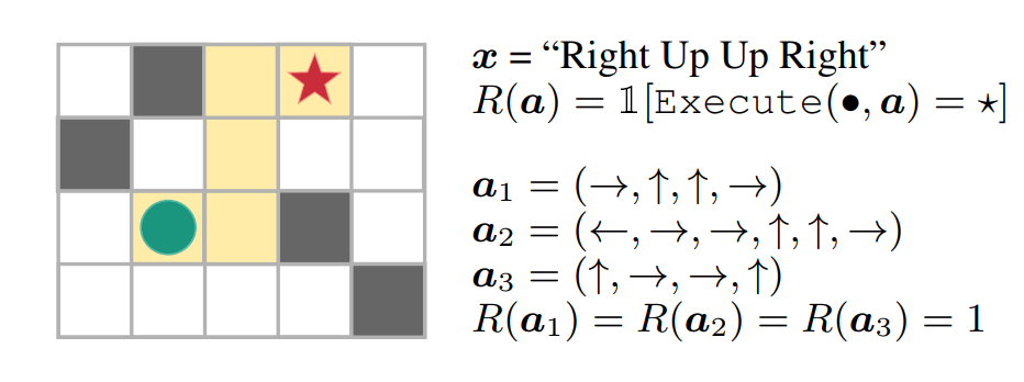
For instance, consider a “blind” agent tasked with reaching a goal position in a maze by following a sequence of natural language commands (e.g., “Right, Up, Up, Right”). Given the input text, the agent (green circle) needs to interpret the commands and take actions based on such interpretation to generate an action sequence (a). The agent receives a reward of 1 if it reaches the goal (red star) and 0 otherwise. Because the agent doesn’t have access to any visual information, the only way for the agent to solve this task and generalize to novel instructions is by correctly interpreting the instructions.

In this instruction-following task, the action trajectories a1, a2 and a3 reach the goal, but the sequences a2 and a3 do not follow the instructions. This illustrates the issue of underspecified rewards.

In these tasks, the RL agent needs to learn to generalize from sparse (only a few trajectories lead to a non-zero reward) and underspecified (no distinction between purposeful and accidental success) rewards. Importantly, because of underspecified rewards, the agent may receive positive feedback for exploiting spurious patterns in the environment. This can lead to reward hacking, causing unintended and harmful behavior when deployed in real-world systems.

In “Learning to Generalize from Sparse and Underspecified Rewards“, we address the issue of underspecified rewards by developing Meta Reward Learning (MeRL), which provides more refined feedback to the agent by optimizing an auxiliary reward function. MeRL is combined with a memory buffer of successful trajectories collected using a novel exploration strategy to learn from sparse rewards. The effectiveness of our approach is demonstrated on semantic parsing, where the goal is to learn a mapping from natural language to logical forms (e.g., mapping questions to SQL programs). In the paper, we investigate the weakly-supervised problem setting, where the goal is to automatically discover logical programs from question-answer pairs, without any form of program supervision. For instance, given the question “Which nation won the most silver medals?” and a relevant Wikipedia table, an agent needs to generate an SQL-like program that results in the correct answer (i.e., “Nigeria”).

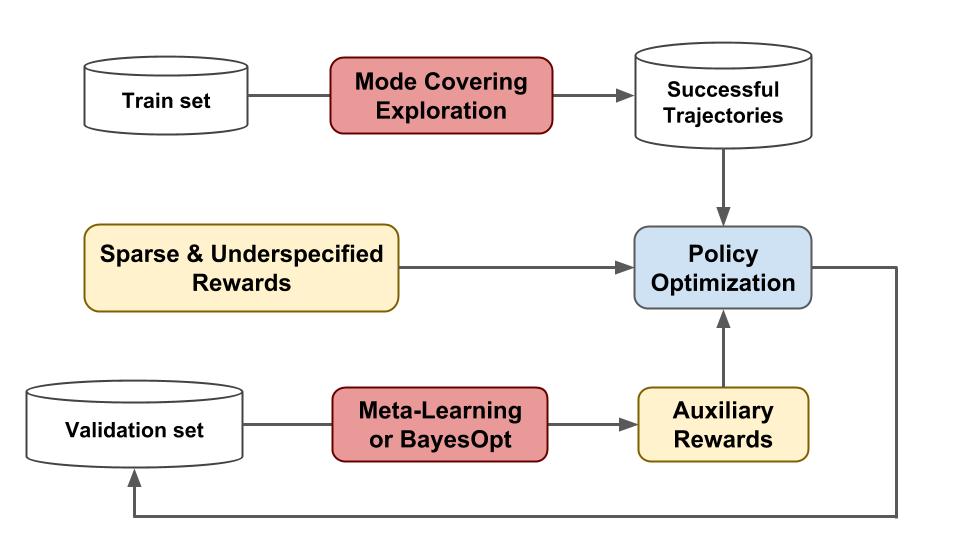
The proposed approach achieves state-of-the-art results on the WikiTableQuestions and WikiSQL benchmarks, improving upon prior work by 1.2% and 2.4% respectively. MeRL automatically learns the auxiliary reward function without using any expert demonstrations, (e.g., ground-truth programs) making it more widely applicable and distinct from previous reward learning approaches. The diagram below depicts a high level overview of our approach:

Overview of the proposed approach. We employ (1) mode covering exploration to collect a diverse set of successful trajectories in a memory buffer; (2) Meta-learning or Bayesian optimization to learn an auxiliary reward that provides more refined feedback for policy optimization.

Meta Reward Learning (MeRL)
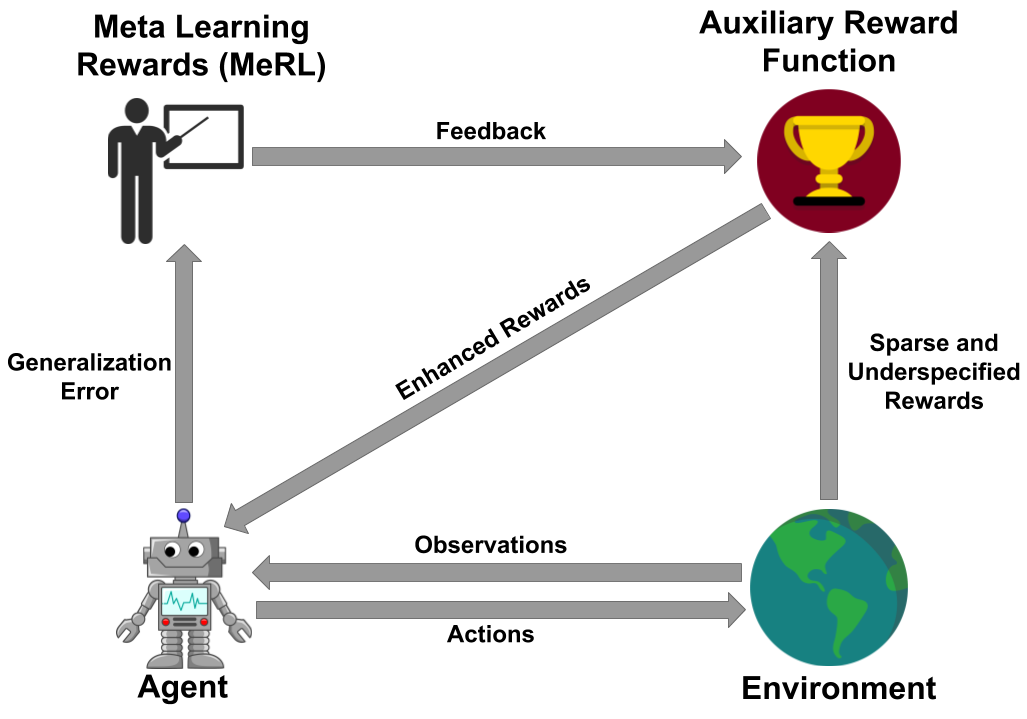
The key insight of MeRL in dealing with underspecified rewards is that spurious trajectories and programs that achieve accidental success are detrimental to the agent’s generalization performance. For example, an agent might be able to solve a specific instance of the maze problem above. However, if it learns to perform spurious actions during training, it is likely to fail when provided with unseen instructions. To mitigate this issue, MeRL optimizes a more refined auxiliary reward function, which can differentiate between accidental and purposeful success based on features of action trajectories. The auxiliary reward is optimized by maximizing the trained agent’s performance on a hold-out validation set via meta learning.

Schematic illustration of MeRL: The RL agent is trained via the reward signal obtained from the auxiliary reward model while the auxiliary rewards are trained using the generalization error of the agent.

Learning from Sparse Rewards
To learn from sparse rewards, effective exploration is critical to find a set of successful trajectories. Our paper addresses this challenge by utilizing the two directions of Kullback–Leibler (KL) divergence, a measure on how different two probability distributions are. In the example below, we use KL divergence to minimize the difference between a fixed bimodal (shaded purple) and a learned gaussian (shaded green) distribution, which can represent the distribution of the agent’s optimal policy and our learned policy respectively. One direction of the KL objective learns a distribution which tries to cover both the modes while the distribution learned by other objective seeks a particular mode (i.e. it prefers one mode over another). Our method exploits the mode covering KL’s tendency to focus on multiple peaks to collect a diverse set of successful trajectories and mode seeking KL’s implicit preference between trajectories to learn a robust policy.

Left: Optimizing mode covering KL. Right: Optimizing mode seeking KL

Conclusion
Designing reward functions that distinguish between optimal and suboptimal behavior is critical for applying RL to real-world applications. This research takes a small step in the direction of modelling reward functions without any human supervision. In future work, we’d like to tackle the credit-assignment problem in RL from the perspective of automatically learning a dense reward function.

Acknowledgements
This research was done in collaboration with Chen Liang and Dale Schuurmans. We thank Chelsea Finn and Kelvin Guu for their review of the paper.

Identifying bird species on the edge using the Amazon SageMaker built-in Object Detection algorithm and AWS DeepLens

Custom object detection has become an important enabler for a wide range of industries and use cases—such as finding tumors in MRIs, identifying diseased crops, and monitoring railway platforms. In this blog post, we build a bird identifier based on an annotated public dataset. This type of model could be used in a number of different ways. You could use it to automate environmental studies for construction projects, or it could be used by bird enthusiasts when bird watching. You could also use this model as a working example to drive new ideas for your own use cases.

For this example, we use the built-in Object Detection algorithm provided by Amazon SageMaker. Amazon SageMaker is an end-to-end machine learning (ML) platform. By using built-in algorithms, developers can accelerate machine learning without needing expertise in using low-level ML frameworks, such as TensorFlow and MXNet. We’ll train the model in Amazon SageMaker’s fully managed and on-demand training infrastructure. Trained models can easily be hosted in the cloud or on the edge using AWS IoT Greengrass.

To demonstrate the use of custom object detection on the edge, we also show you how to deploy the trained model on AWS DeepLens, the world’s first deep-learning-enabled video camera for developers. AWS DeepLens helps put deep learning in the hands of developers, literally, with a fully programmable video camera, tutorials, code, and pre-trained models designed to expand deep learning skills.

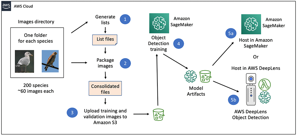
The following diagram gives a high-level view how our bird identifier solution is built:

Understanding the dataset

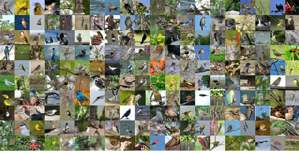
The CUB 200-2011 birds dataset contains 11,788 images across 200 bird species (the original technical report can be found here). Each species comes with about 60 images, with a typical size of about 350 pixels by 500 pixels. Bounding boxes are provided, as are annotations of bird parts. A recommended train/test split is given, but image size data is not.

Preparing the image dataset

The most efficient way to provide image data to the Amazon SageMaker Object Detection algorithm is by using the RecordIO format. MXNet provides a tool called im2rec.py to create RecordIO files for your datasets. To use the tool, you provide listing files describing the set of images.

For object detection datasets, Amazon SageMaker needs bounding boxes to be described in terms of xmin, ymin, xmax, and ymax, which are ratios of the box corners to the full image. The CUB dataset bounding box instead gives you x, y, width, and height in pixels. See the following picture to understand the difference in metadata.

To address this discrepancy, we retrieve the size of each image and translate the absolute bounding box to have dimensions relative to the image size. In the following example, the box dimensions from the dataset are shown in black, while the dimensions required by RecordIO are shown in green.

The following Python code snippet shows how we converted the original bounding box dimensions to those needed by im2rec. See the sample Amazon SageMaker notebook for the full code.

# Define the bounding boxes in the format required by the Amazon SageMaker 
# built-in Object Detection algorithm.
# The xmin/ymin/xmax/ymax parameters are specified as ratios to 
# the total image pixel size

df['header_cols'] = 2 # number of header cols and label width
df['label_width'] = 5 # label cols: class, xmin, ymin, xmax, ymax

df['xmin'] =  df['x_abs'] / df['width']
df['xmax'] = (df['x_abs'] + df['bbox_width']) / df['width']
df['ymin'] =  df['y_abs'] / df['height']
df['ymax'] = (df['y_abs'] + df['bbox_height']) / df['height']

With the listing files in place, the im2rec utility can be used to create the RecordIO files by executing the following command:

python im2rec.py --resize 256 --pack-label birds CUB_200_2011/images/

After the RecordIO files are created, they are uploaded to Amazon S3 as input to the Object Detection algorithm with the following Python code:

train_channel      = prefix + '/train'
validation_channel = prefix + '/validation'

sess.upload_data(path='birds_ssd_sample_train.rec',
                 bucket=bucket,
                 key_prefix=train_channel)
sess.upload_data(path='birds_ssd_sample_val.rec',
                 bucket=bucket,
                 key_prefix=validation_channel)

Training the object detection model using the Amazon SageMaker built-in algorithm

With the images available in Amazon S3, the next step is to train the model. Documentation for the object detection hyperparameters is available here. For our example, we have a few hyperparameters of interest:

  • Number of classes and training samples.
  • Batch size, epochs, image size, pre-trained model, and base network.

Note that the Amazon SageMaker Object Detection algorithm requires models to be trained on a GPU instance type such as ml.p3.2xlarge. Here is a Python code snippet for creating an estimator and setting the hyperparameters:

od_model = sagemaker.estimator.Estimator(
                 training_image,
                 role, 
                 train_instance_count=1, 
                 train_instance_type='ml.p3.2xlarge',
                 train_volume_size = 50,
                 train_max_run = 360000,
                 input_mode= 'File',
                 output_path=s3_output_location,
                 sagemaker_session=sess)  

od_model.set_hyperparameters(
                 base_network='resnet-50',
                 use_pretrained_model=1,
                 num_classes=5,
                 mini_batch_size=16,
                 epochs=100,               
                 learning_rate=0.001, 
                 lr_scheduler_step='33,67',
                 lr_scheduler_factor=0.1,
                 optimizer='sgd',
                 momentum=0.9,
                 weight_decay=0.0005,
                 overlap_threshold=0.5,
                 nms_threshold=0.45,
                 image_shape=512,
                 label_width=350,
                 num_training_samples=150)

With the dataset uploaded, and the hyperparameters set, the training can be started using the following Python code:

s3_train_data      = 's3://{}/{}'.format(bucket, train_channel)
s3_validation_data = 's3://{}/{}'.format(bucket, validation_channel)

train_data      = sagemaker.session.s3_input(
                         s3_train_data,
                         distribution='FullyReplicated',
                         content_type='application/x-recordio',
                         s3_data_type='S3Prefix')
validation_data = sagemaker.session.s3_input(
                         s3_validation_data,
                         distribution='FullyReplicated',
                         content_type='application/x-recordio',
                         s3_data_type='S3Prefix')

data_channels = {'train': train_data, 'validation': validation_data}

od_model.fit(inputs=data_channels, logs=True)

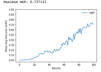
For a subset of 5 species on an ml.p3.2xlarge instance type, we can get accuracy of 70 percent or more with 100 epochs in about 11 minutes.

You can create the training job using the AWS CLI, using a notebook, or using the Amazon SageMaker console.

Hosting the model using an Amazon SageMaker endpoint

After we have trained our model, we’ll host it on Amazon SageMaker. We use CPU instances, but you can also use GPU instances. Deployment from your Amazon SageMaker notebook takes a single line of Python code:

object_detector = od_model.deploy(
                     initial_instance_count = 1,
                     instance_type = 'ml.m4.xlarge')

Testing the model

After the model endpoint is in service, we can pass in images that the model has not yet seen and see how well the birds are detected. See the sample notebook for a visualize_detections function. Given a URL to a bird image, here is the Python code to invoke the endpoint, get back a set of predicted bird species and their bounding boxes, and visualize the results:

b = ''
with open(filename, 'rb') as image:
    f = image.read()
    b = bytearray(f)

endpoint_response = runtime.invoke_endpoint(
                                 EndpointName=ep,
                                 ContentType='image/jpeg',
                                 Body=b)
results    = endpoint_response['Body'].read()
detections = json.loads(results)

visualize_detection(filename,
                    detections['prediction'],
                    OBJECT_CATEGORIES, thresh)

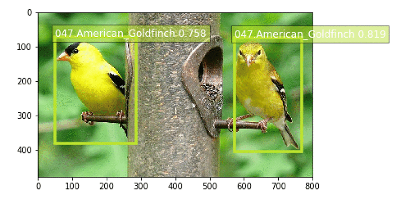
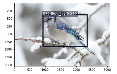
Here is a sample result for an image of a blue jay:

Running your model on the edge using AWS DeepLens

In some use cases, an Amazon SageMaker hosted endpoint will be a sufficient deployment mechanism, but there are many use cases that require real-time object detection at the edge. Imagine a phone-based assistant app in a bird sanctuary. You walk around and point your app at a bird and instantly get details about the species (listen to the bird call, understand its habitat, etc.). No more guessing about what bird you just saw.

AWS DeepLens lets you experiment with deep learning on the edge, giving developers an easy way to deploy trained models and use Python code to come up with interesting applications. For our bird identifier, you could mount an AWS DeepLens device next to your kitchen window overlooking a set of bird feeders. The device could feed cropped images of detected birds to Amazon S3. It could even trigger a text to your mobile phone to let you know what birds visited.

A previous blog post  covered how to deploy a custom image classification model on AWS DeepLens. For a custom object detection model, there are two differences:

  • The model artifacts must be converted before being deployed.
  • The model must be optimized before being loaded.

Let’s go into more detail on each of these differences.

Convert your model artifacts before deploying to AWS DeepLens

For custom object detection models produced by Amazon SageMaker, you need to perform an additional step if you want to deploy your models on AWS DeepLens. MXNet provides a utility function for converting the model. To get started with conversion, first clone the GitHub repository:

git clone https://github.com/apache/incubator-mxnet

The next step is to download a copy of your model artifacts that were saved in Amazon S3 as a result of your training job. Extract the actual artifacts (a parameters file, a symbol file, and the hyperparameters file), and rename them so that they reflect the base network and the image size that were used in training. Here are the commands from a bash script you can use to perform the conversion:

BUCKET_AND_PREFIX=s3://<your-bucket>/<your-prefix>/output
TARGET_PREFIX=s3://<your-deeplens-bucket>/<your-prefix>
rm -rf tmp && mkdir tmp
aws s3 cp $BUCKET_AND_PREFIX/model.tar.gz tmp
gunzip -k -c tmp/model.tar.gz | tar -C tmp -xopf –
mv tmp/*-0000.params tmp/ssd_resnet50_512-0000.params
mv tmp/*-symbol.json tmp/ssd_resnet50_512-symbol.json

After the contents have been extracted and renamed, invoke the conversion utility:

python incubator-mxnet/example/ssd/deploy.py --network resnet50 
  --data-shape 512 --num-class 5 --prefix tmp/ssd_

You can now remove the original files and create a new compressed tar file with the converted artifacts.  Copy the new model artifacts file to Amazon S3, where it can be used when importing a new AWS DeepLens object detection model:

rm tmp/ssd_* && rm tmp/model.tar.gz
tar -cvzf ./patched_model.tar.gz -C tmp 
  ./deploy_ssd_resnet50_512-0000.params 
  ./deploy_ssd_resnet50_512-symbol.json 
  ./hyperparams.json
aws s3 cp patched_model.tar.gz $TARGET_PREFIX-patched/

Note that the destination bucket for the patched model must have the word “deeplens” in the bucket name. Otherwise, you will get an error when importing the model in the AWS DeepLens console. A complete script for patching the model artifacts can be found here.

Optimize the model from your AWS Lambda function on AWS DeepLens

An AWS DeepLens project consists of a trained model and an AWS Lambda function. Using AWS IoT Greengrass on the AWS DeepLens, the inference Lambda function performs three important functions:

  • It captures the image from a video stream.
  • It performs an inference using that image against the deployed machine learning model.
  • It provides the results to both AWS IoT and the output video stream.

AWS IoT Greengrass lets you execute AWS Lambda functions locally, reducing the complexity of developing embedded software. For details on creating and publishing your inference Lambda function, see this documentation.

When using a custom object detection model produced by Amazon SageMaker, there is an additional step in your AWS DeepLens inference Lambda function. The inference function needs to call MXNet’s model optimizer before performing any inference using your model. Here is the Python code for optimizing and loading the model:

ret, model_path = mo.optimize('deploy_ssd_resnet50_512',
                              input_width, input_height)
model = awscam.Model(model_path, {'GPU': 1})

Performing model inference on AWS DeepLens

Model inference from your AWS Lambda function is very similar to the steps we showed earlier for invoking a model using an Amazon SageMaker hosted endpoint. Here is a piece of the Python code for finding birds in a frame provided by the AWS DeepLens video camera:

frame_resize = cv2.resize(frame, (512, 512))

# Run the images through the inference engine and parse the results using
# the parser API.  Note it is possible to get the output of doInference
# and do the parsing manually, but since it is a ssd model,
# a simple API is provided.
parsed_inference_results = model.parseResult(
                                 model_type,
                                 model.doInference(frame_resize))

A complete inference Lambda function for use on AWS DeepLens with this object detection model can be found here.

Conclusion

In this blog post, we have shown how to use the Amazon SageMaker built-in Object Detection algorithm to create a custom model for detecting bird species based on a publicly available dataset. We also showed you how to run that model on a hosted Amazon SageMaker endpoint and on the edge using AWS DeepLens. You can clone and extend this example for your own use cases. We would love to hear how you are applying this code in new ways. Please let us know your feedback by adding your comments.


About the author

Mark Roy is a Solution Architect focused on Machine Learning, with a particular interest in helping customers and partners design computer vision solutions.  In his spare time, Mark loves to play, coach, and follow basketball.


On the Path to Cryogenic Control of Quantum Processors

Building a quantum computer that can solve practical problems that would otherwise be classically intractable due to the computation complexity, cost, energy consumption or time to solution, is the longstanding goal of the Google AI Quantum team. Current thresholds suggest a first generation error-corrected quantum computer will require on the order of 1 million physical qubits, which is more than four orders of magnitude more qubits than exist in Bristlecone, our 72 qubit quantum processor. Increasing the number of physical qubits needed for a fault-tolerant quantum computer while maintaining high-quality control of each qubit are intertwined and exciting technological challenges that will require inventions beyond simply copying and pasting our current control architecture. One critical challenge is reducing the number of input/output control lines per qubit by relocating the room temperature analog control electronics to the 3 kelvin stage in the cryostat, while maintaining high-quality qubit control.

As a step towards solving that challenge, this week we presented our first generation cryogenic-CMOS single-qubit controller at the International Solid State Circuits Conference in San Francisco. Fabricated using commercial CMOS technology, our controller operates at 3 kelvin, consumes less than 2 milliwatts of power and measures just 1 mm by 1.6 mm. Functionally, it provides an instruction set for single-qubit gate operations, providing analog control of a qubit via digital lines between room temperature and 3 kelvin, all while consuming ~1000 times less power compared to our current room temperature control electronics.

Google’s first generation cryogenic-CMOS single-qubit controller (center and zoomed on the right) packaged and ready to be deployed inside our cryostat. The controller measures 1mm by 1.6mm.

How to Control 72 Qubits
In our lab in Santa Barbara, we run programs on Bristlecone by applying gigahertz frequency analog control signals to each of the qubits to manipulate the qubit state, to entangle qubits and to measure the outcomes of our computations. How well we define the shape and frequency of these control signals directly impacts the quality of our computation. To make high-quality qubit control signals, we leverage technology developed for smartphones packaged in server racks at room temperature. Individual coaxial cables deliver these signals to each qubit, which are themselves kept inside a cryostat chilled to 10 millikelvin. While this approach makes sense for a Bristlecone-scale quantum processor, which demands 2 control lines per qubit for 144 unique control signals, we realized that a more integrated approach would be required in order to scale our systems to the million qubit level.

Research Scientist Amit Vainsencher checking the wiring on Bristlecone in one of Google’s flagship cryostats. Blue coaxial cables are connected from custom analog control electronics (server rack on the right) to the quantum processor.

In our current setup, the number of physical wires connected from room temperature to the qubits inside the cryostat and the finite cooling power of the cryostat represent a significant constraint. One way to alleviate this is to move the digital to analog control closer to the quantum processor. Currently, our room temperature digital-to-analog waveform generators used to control individual qubits, dissipate ~1 watt of waste heat per qubit. The cooling power of our cryostat at 3 kelvin is 0.1 watt. That means if we crammed 150 waveform generators into our cryostat (never mind the limited physical space inside the refrigerator for a moment) we would overwhelm the cooling power of our cryostat by 1500x, thereby cooking our cryostat and rendering our qubits useless. Therefore, simply installing our existing digital-to-analog control in the cryostat will not set us on the path to control millions of qubits. It is clear we need an integrated low-power qubit control solution.

A Cool Idea
In collaboration with University of Massachusetts Professor Joseph Bardin, we set out to develop custom integrated circuits (ICs) to control our qubits from within the cryostat to ultimately reduce the physical I/O connections to and from our future quantum processors. These ICs would be designed to operate in the ultracold environment, specifically 3 kelvin, and turn digital instructions into analog control pulses for qubits. A key research objective was to first design a custom IC with low power requirements, in order to prevent warming up the cryostat.

We designed our IC to dissipate no more than 2 milliwatts of power at 3 kelvin, which can be challenging as most physical CMOS models assume operation closer to 300 kelvin. After design and fabrication of the IC with the low power design constraints in mind, we verified that the cryogenic-CMOS qubit controller worked at room temperature. We then mounted it in our cryostat at 3 kelvin and connected it to a qubit (mounted at 10 millikelvin in the same cryostat). We carried out a series of experiments to establish that the cryogenic-CMOS qubit controller worked as designed, and most importantly, that we hadn’t just installed a heater inside our cryostat.

Schematic of the cryogenic-CMOS qubit controller mounted on the 3 kelvin stage of our dilution refrigerator and connected to a qubit. Our standard qubit control electronics were connected in parallel to enable control and measurement of the qubit as an in-situ check experiment.

Performance at Low Temperature
Baseline experiments for our new quantum control hardware, including T1, Rabi oscillations, and single qubit gates, show similar performance compared to our standard room-temperature qubit control electronics: qubit coherence time was virtually unchanged, and high-visibility Rabi oscillations were observed by varying the amplitude of the pulses out of the cryogenic-CMOS qubit controller—a signature response of a driven qubit.

Comparison of the qubit coherence time measured using the standard and cryogenic quantum controllers.
Measured Rabi amplitude oscillations using the cryogenic controller. The green and black traces are the probability of measuring the qubits in the 1 and 0 states, respectively.

Next Steps
Although all of these results are promising, this first generation cryogenic-CMOS qubit controller is but one small step towards a truly scalable qubit control and measurement system. For instance, our controller is only able to address a single qubit, and it still requires several connections to room temperature. In addition, we still need to work hard to quantify the error rates for single qubit gates. As such, we are excited to reduce the energy required to control qubits and still maintain the delicate control required to perform high-quality qubit operations.

Acknowledgements
This work was carried out with the support of the Google Visiting Researcher Program while Prof. Bardin, an Associate Professor with the University of Massachusetts Amherst, was on sabbatical with the Google AI Quantum Team. This work would not have been possible without the many contributions of members of the Google AI Quantum team, especially Evan Jeffrey for his integration of the cryo-CMOS controller into the qubit calibration software, Ted White for his on-demand qubit calibrations and Trent Huang for his tireless design rules checks.

Machine learning for MEG during speech tasks

Vector Faculty Member, Frank Rudzicz, calls language a “lens into one’s cognition” because how and what we say can reveal a lot about how we feel, and how we think. In research recently published in the scientific journal Nature, Rudzicz and his PhD student at Vector, Demetres Kostas and collaborator Elizabeth Pang, consider how one’s brain signals can provide a lens into how we speak.

Specifically, the team considered whether a deep neural network trained with monitored brain signals can be used to predict the ages of 92 children (aged 4-18) performing speech tasks, such as verb generation and specified babble. This used a technology called magnetoencephalography (MEG) – a massive device that gently reads signals in the brain using 151 sensors to record data across various locations on the scalp while a person speaks. The results were able to achieve 95% accuracy on a binary task identifying the age of the speaker from their brain signals alone and suggest that the deep neural network makes predictions based on differences in speech development – how healthy kids learn to speak as revealed by their brain signals. In this research, the team also highlighted the differences between traditional machine learning, and modern deep methods on performing tasks such as this.

This work is the first step towards understanding how speech originates in the brain. While the next steps are still fairly theoretical, Demetres and the team are interested in applying methods from ‘explainable AI’ to making the interpretation of brain signals more understandable to clinicians and researchers. Being able to map healthy speech production will have a variety of uses, including helping people who have difficulty speaking through computer interfaces.


Check out the full paper here: Machine learning for MEG during speech tasks

Newstag improves global video news discoverability using AI language services on AWS

Swedish startup Newstag uses artificial intelligence (AI) to allow customers to create personalized video news channels from major global news providers. Their mission is to continuously empower people and organizations with the latest, diverse information. To increase discoverability of video news from all around the world for their customers, Newstag creates rich metadata for each video. Newstag was able to automate this manually intensive process of extracting and creating metadata from videos by using Amazon Transcribe, Amazon Translate, and Amazon Comprehend. Using a combination of AWS services, Newstag can create rich metadata for ten times more videos than was previously possible.

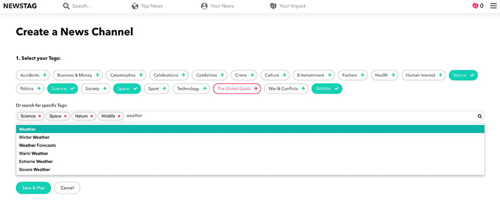
“We believe people want to choose what news they want to see. Enabling customers to curate relevant stories is pivotal for us to carry out our company mission,” says Mats Ekholm, Chief Technology Officer of Newstag. To accomplish this, Newstag has developed tags that customers can select to create a personalized video news channel. The following screenshot illustrates how customers can select these tags in Newstag.

To curate over 1,000 videos a day, Newstag’s editorial staff had spent a lot of time manually tagging content in various languages. Tags mostly consisted of titles, brief descriptions, and limited metadata. Struggling to keep up with demand, the startup looked for a simple, cost-efficient, and easy-to-deploy solution. By using pre-trained machine learning (ML) services on AWS, Newstag was able to use AI to solve the problem even though they had no previous experience with the technology.

First, Newstag uses Amazon Transcribe to create transcripts of speech in supported languages from the videos stored using Amazon Simple Storage Service (S3). Then Amazon Translate is applied to non-English transcripts as well as other titles, descriptions, or keywords originally provided with the video for accurate translation into English. Finally, Amazon Comprehend, a machine learning service that provides insights from analyzing textual content, is used to extract entities from all texts available in English. These named entities, such as organizations, people, places, and locations, are used to create accurate tags to help customers find targeted content.

“We used to manually create tags for about three to four videos per hour,” explains Ekholm. “With AI language services offered by AWS, we can now create tags for about 30 to 40 videos per hour. It means a 10-times increase in the number of news stories that our customers can see on Newstag.”

Ekholm automated a majority of the tagging process for video news in different languages within five hours at low cost. “I was impressed by how easy it was to deploy Transcribe, Translate, and Comprehend. I was also very pleased with their low costs. As a start-up, we have to be smart about operating costs,” says Ekholm.

Learn more

See the AWS website to learn more about language services for AI. Here are some useful blog posts from AWS to get you started:


About the Author

Woo Kim is a Product Marketing Manager for AWS machine learning services. He spent his childhood in South Korea and now lives in Seattle, WA. In his spare time, he enjoys playing volleyball and tennis.



Run ONNX models with Amazon Elastic Inference

At re:Invent 2018, AWS announced Amazon Elastic Inference (EI), a new service that lets you attach just the right amount of GPU-powered inference acceleration to any Amazon EC2 instance. This is also available for Amazon SageMaker notebook instances and endpoints, bringing acceleration to built-in algorithms and to deep learning environments.

In this blog post, I show how to use the models in the ONNX Model Zoo on GitHub to perform inference by using MXNet with Elastic Inference Accelerator (EIA) as a backend.

The benefits of Amazon Elastic Inference

Amazon Elastic Inference allows you to attach low-cost GPU-powered acceleration to Amazon EC2 and Amazon SageMaker instances to reduce the cost of running deep learning inference by up to 75 percent.

Amazon Elastic Inference provides support for Apache MXNet, TensorFlow, and ONNX models. ONNX is an open standard format for deep learning models that enables interoperability between deep learning frameworks such as Apache MXNet, Caffe2, Microsoft Cognitive Toolkit (CNTK), PyTorch, and more. This means that you can use any of these frameworks to train a model, export the model in ONNX format, and then import them into Apache MXNet for inference.

You can see the collection of pre-trained, state-of-the-art models in ONNX format at the ONNX Model Zoo on GitHub.

Getting started with inference by using Resnet 152v1 model

To start with the tutorial, I use an AWS Deep Learning AMI (DLAMI), which already provides support for Apache MXNet, EIA, ONNX and other required libraries. You can review Elastic Inference Prerequisites for the instructions related to Elastic Inference. For detailed instructions on how to launch a DLAMI with an Elastic Inference Accelerator, see the Elastic Inference documentation. I use the standard ResNet-152v1 ONNX model from model zoo for inference in MXNet.

Step 1: Activate the MXNet EI environment

To begin the tutorial, log in to your Deep Learning AMI with Conda console. Activate the Python 3 MXNet EI environment.

source activate amazonei_mxnet_p36

Step 2: Import dependencies and download

From the ONNX model zoo, download both the Resnet-152v1 model and synset.txt file, which contains class labels.

import mxnet as mx
import matplotlib.pyplot as plt
import numpy as np
from mxnet.gluon.data.vision import transforms
from mxnet.contrib.onnx.onnx2mx.import_model import import_model
import os
# Download model and synset.txt files containing class labels
mx.test_utils.download('https://s3.amazonaws.com/onnx-model-zoo/resnet/resnet152v1/resnet152v1.onnx')
mx.test_utils.download('https://s3.amazonaws.com/onnx-model-zoo/synset.txt')
with open('synset.txt', 'r') as f:
    labels = [l.rstrip() for l in f]

# Download image for inference
img_path = mx.test_utils.download('https://s3.amazonaws.com/onnx-mxnet/examples/mallard_duck.jpg')

Step 3: Import ONNX model in MXNet and perform inference

Import ONNX model in MXNet with the help of ONNX-MXNet API.

# Enter path to the ONNX model file
model_path= 'resnet152v1.onnx'
sym, arg_params, aux_params = import_model(model_path)

Load the resnet152v1 network for inference using CPU context.

# Determine and set context
ctx = mx.cpu()
# Load module
mod = mx.mod.Module(symbol=sym, context=ctx, label_names=None)
mod.bind(for_training=False, data_shapes=[('data', (1,3,224,224))], 
         label_shapes=mod._label_shapes)
mod.set_params(arg_params, aux_params, allow_missing=True, allow_extra=True)

Define a predict function, which takes the path of the input image and prints the top five predictions.

# Preprocess input image
def preprocess(img):   
    transform_fn = transforms.Compose([
    	transforms.Resize(256),
    	transforms.CenterCrop(224),
    	transforms.ToTensor(),
    	transforms.Normalize([0.485, 0.456, 0.406], [0.229, 0.224, 0.225])
    ])
    img = transform_fn(img)
    img = img.expand_dims(axis=0)
    return img

def predict(path):
    img = preprocess(path)
    # Run forward pass
    mod.predict(mx.nd.array(img))
    # Take softmax to generate probabilities
    scores = mx.ndarray.softmax(mod.get_outputs()[0]).asnumpy()
    # print the top-5 inferences class
    scores = np.squeeze(scores)
    a = np.argsort(scores)[::-1]
    for i in a[0:5]:
        print('class=%s ; probability=%f' %(labels[i],scores[i]))

Plot the input image for inference.

img = mx.image.imread(img_path)
plt.imshow(img.asnumpy())

Step 4: Generate prediction on input image

The top five classes, in order, along with the probabilities generated for the image displayed are as below.

predict(img)

Result:
class=n01847000 drake ; probability=0.999519
class=n02018207 American coot, marsh hen, mud hen, water hen, Fulica americana ; probability=0.000230
class=n01855032 red-breasted merganser, Mergus serrator ; probability=0.000130
class=n01855672 goose ; probability=0.000044
class=n09332890 lakeside, lakeshore ; probability=0.000022

Evaluate your output and improve performance

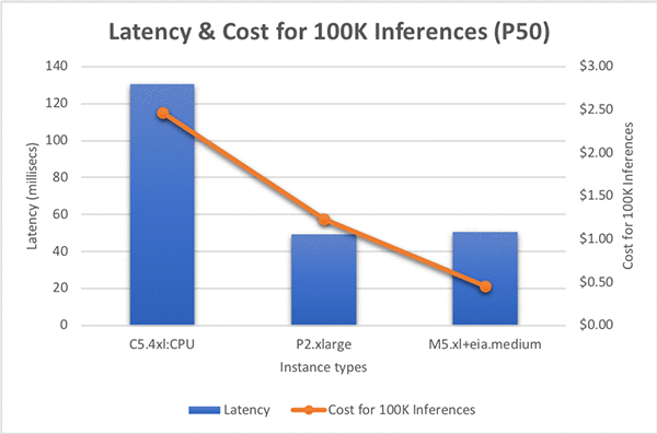
Inference on this model takes approximately 131 milliseconds on C5.4xlarge. So, for 100,000 inference requests, this would cost $2.46 USD. This can be expensive for production use cases. So, let’s look at how Amazon Elastic Inference can help.

Amazon Elastic Inference is available in the following three sizes, making it efficient for a wide range of inference models including computer vision, natural language processing, and speech recognition.

  • eia1.medium: 8 teraflops of mixed-precision performance
  • eia1.large: 16 teraflops of mixed-precision performance
  • eia1.xlarge: 32 teraflops of mixed-precision performance

This lets you select the best price-to-performance ratio for your application. I ran the inference on the same model using GPU and EIA contexts to see the difference in the cost and performance.

To run the model with mx.eia() context, you just need to do minor changes in the code.

  1. With EIA context, when you use either the Symbol API or the Module API, make sure you set for_training=False.
  2. Set the context to bind your model as ctx=mx.eia().

EI typically aims to minimize the host instance CPU memory requirements by offloading to the EI accelerator, but some pre and post-processing must still be done on the host. Depending on the application’s compute and memory requirements, you can select the instance types that are most appropriate.

I evaluated performance of this model with C5 and M5 instances but found that this model required more CPU memory. The M5 instances with more RAM were the most cost effective solution. I ran tests with a few different sized M5 instances with an EIA1.Medium accelerator and observed that instance sizes larger than the M5.xlarge didn’t materially improve latency performance. Next, I tested the M5.xlarge with different EI accelerator sizes. Inference calls with an EIA1.large accelerator were significantly faster than an EIA1.Medium, but my EIA1.Medium at 50ms for an inference request met my requirements, so I didn’t need more horsepower.

Based on my requirements, I decided on an M5.xlarge with an EIA1.Medium as the right infrastructure combination for my workload. Comparing the hourly costs for the instances in our comparison: a P2.xlarge cost $0.90 per hour, whereas the M5.xlarge + EIA1.Medium costs $0.32 per hour, and lastly the C5.4xlarge is $0.68 per hour. But let’s also compare the cost to perform 100,000 inferences, this will incorporate hourly cost and performance to give us a meaningful comparison. The P2.xlarge costs $1.23 to execute 100,000 inferences, whereas this new EI based combination costs $0.45, a whopping 74% reduction in cost, sacrificing just 2% speed. If you use C5.4xlarge, it costs $2.47 and is 2.5x slower than M5.xlarge with EIA1.Medium! See the graph below for more information:

Conclusion

As you can see from the tutorial here, Amazon Elastic Inference gives you the opportunity to select the best price-to-performance ratio suitable for your application. For ONNX ResNet152 model inference, EIA1.medium is 2.5x faster and 81% cheaper than C5.4xlarge! Also with ONNX support, you can export models trained in different deep learning frameworks to run inference with EIA using Apache MXNet as a backend.

For general information about how to use EI, see Working with Amazon EI in the EC2 user guide. You can also find more information about ONNX support in MXNet, in the ONNX API documentation on the MXNet website.


About the Authors

Roshani Nagmote is a Software Developer for AWS Deep Learning. She focusses on building distributed Deep Learning systems and innovative tools to make Deep Learning accessible for all. In her spare time, she enjoys hiking, exploring new places and is a huge dog lover.


Vandana Kannan is a Software Developer for AWS Deep Learning focusing on building scalable deep learning systems. In her spare time, she enjoys painting, learning Indian classical dance, and spending time with family and friends.



Hagay Lupesko is an Engineering Manager for AWS Deep Learning. He focuses on building Deep Learning tools that enable developers and scientists to build intelligent applications. In his spare time he enjoys reading, hiking and spending time with his family.