Blog

Learn About Our Meetup

5000+ Members

MEETUPS

LEARN, CONNECT, SHARE

Join our meetup, learn, connect, share, and get to know your Toronto AI community. 

JOB POSTINGS

INDEED POSTINGS

Browse through the latest deep learning, ai, machine learning postings from Indeed for the GTA.

CONTACT

CONNECT WITH US

Are you looking to sponsor space, be a speaker, or volunteer, feel free to give us a shout.

Author: torontoai

Machine learning: What’s in it for government?

Machine learning (ML) allows governments to deliver better, more cost-effective, and citizen-friendly services. We talked with three Amazon Web Services (AWS) customers from government authorities and institutes who shared their stories about how ML helped them transform their services and their organizations. These customers gathered at an executive learning track curated particularly for European Government delegates, as part of AWS re:Invent 2018.

The National Health Service Business Services Authority

The United Kingdom’s (UK) National Health Service Business Services Authority (NHSBSA), the organization overseeing the delivery of primary care, dental and prescription services to UK citizens, told us how they introduced Amazon Connect, a cloud-based chatbot to its contact center service to increase its capacity to respond to customer needs.

Chris Suter, Lead Cloud Architect of Digitisation, Insight, and Technology Solutions, shared the results of this investment with the group. In the first three weeks of its implementation, the chatbot helped NHSBSA respond to approximately 11,000 calls, addressing simple queries and rerouting complicated queries to staff who can provide more support. This helped NHSBSA save USD $650,000 per year.

NHSBSA used Amazon Lex to ensure that the calls were routed automatically and answered correctly, and they used Amazon Polly to simulate human-like speech. The ML-powered front end handles 40 percent of inbound calls, making staff available with an almost-zero customer queue time.

“This not only resulted in higher efficiency and cost savings for NHSBSA, but also boosted the morale of employees as they could focus their efforts on providing adequate guidance to customers with more complicated questions,” Suter said.

The Belgian public employment service VDAB

Another AWS customer, Belgian public employment service VDAB, wanted to know how they could use machine learning to improve job-matching, that is  finding the right opportunities for the right people. Radix.ai’s JobNet used a deep learning model to enhance this function. With each new dataset, the engine learns how the job market evolves, noting changes in job demand and how trends shift over time.

The deep learning model goes beyond analysis of words in job descriptions and resumes to include information on interests and talents of job seekers. By using this service, employment officials want to provide better and faster connections between job seekers and available jobs.

The Royal Institute of Blind People

The impact of machine learning on people with disabilities has also been transformative. The Royal Institute of Blind People (RNIB) uses Amazon Polly to provide the UK’s largest community of blind and partially sighted people with reading services. RNIB’s Talking Books service provides access to over 26,000 audiobooks, free of charge. For millions of people in the UK, this service can be life changing.

More and more government customers are discovering that ML can be a game-changing technology for their users, and in turn for their businesses. These examples serve as starting points for governments.

About the AWS Institute

The AWS Institute, which curated this program, will publish more blog posts on how machine learning has an impact on the public sector.

The AWS Institute convenes global leaders who share an interest in solving some of the world’s most pressing challenges using technology. The Institute convenes leaders from government, academia, and nonprofit organizations for private discussions to explore innovative ideas to transform the public sector. For a related blog post on how to prepare governments for digital transformation, check out How Can Government Grow and Recruit Digital Talent? The Case of the UK Driver and Vehicle Licensing Agency.


About the Author

Maysam Ali is Global Content Lead for the Amazon Web Services Institute. She writes about the impact of technology on society. She helps governments, nonprofits and educational leaders better understand how they can use new technologies, including machine learning and artificial intelligence, to address major societal challenges.


Leonardo Quattrucci is the Lead for Europe, Middle East and Africa for the Amazon Web Services Institute. He works with government executives to accelerate public sector transformation. By innovating on policy processes and building digital competencies, he is helping leaders use technology to deliver better citizen services.


Creating hierarchical label taxonomies using Amazon SageMaker Ground Truth

At re:Invent 2018 we launched Amazon SageMaker Ground Truth, which can Build Highly Accurate Datasets and Reduce Labeling Costs by up to 70% using machine learning. Amazon SageMaker Ground Truth offers easy access to public and private human labelers and provides them with built-in workflows and interfaces for common labeling tasks. Additionally, Amazon SageMaker Ground Truth lowers your labeling costs by using automated data labeling, which works by training Ground Truth from data labeled by humans so that the service learns to label data independently.

Let’s suppose we have a large corpus of images taken from cameras on a street. Each image might contain many different objects important for developing algorithms for driverless cars (e.g., vehicles or traffic signals). We must first define a hierarchical representation of the information that we want to capture from the images (see below for an example of what such a label taxonomy may look like). We then begin the labeling process by taking these raw, unlabeled images and labeling them with the high-level classes (e.g., ‘vehicles’, ‘traffic-signals’, and ‘pedestrian’.

In this blog post, we’ll show you how to accomplish such hierarchical labeling with Amazon SageMaker Ground Truth by chaining jobs and making use of the augmented manifest functionality.

How is this typically solved?

In supervised machine learning, we typically use a labeled dataset that contains both the raw data and the associated label for each data object. For example, you can have a training dataset of street images and classify them into “traffic-signals” or “no-traffic-signals” (where the label 0 and 1 correspond to the two classes). These labels are usually stored in a formats, such as CSV or JSON with the first column representing the raw data and the second column representing the label.

However, if you want to further label the same set of images (for example, to identify the type of traffic signals in the “traffic-signals” set), we typically create a new dataset by performing a filtering operation on the first dataset to select only those images with traffic signals in them. This reduces the dataset into another subset containing only “traffic-signals” (label 0) in it. Then we can add new label to classify traffic signals as ‘stop-sign’, ‘speed-limit’, and so on.

These kinds of filtering operations might become costly and time-consuming for large datasets. We might also want to mark all the stop signs and pedestrians in an image by an object detection (bounding box) algorithm. This typically requires us to create a third dataset by adding object detection labels around each of the stop signs and pedestrians in it. You can see that, as we continue classifying deep into the taxonomy, the number and complexity of the training datasets increases at approximately same rate as the fanout factor of the taxonomy (exponential in the most complex case).

In short when working with a hierarchical taxonomy, you need to be able to do all of the following:

  1. Associate multiple layers of labels to an image, and be able to store and retrieve them efficiently and cost effectively.
  2. Create a filtered dataset containing a given label efficiently and cost effectively.
  3. Train a model for a given label in the dataset containing multiple labels.

Amazon SageMaker Ground Truth helps you accomplish these tasks easily using the job chaining and augmented manifest functionality.

Job chaining

When you label datasets, often there will be different types of labels (image classification, bounding boxes, semantic segmentation, etc.) that might require a different UI or dramatically different labeling context that would in turn require different instructions for the labelers for optimal quality. In such cases, it can become necessary to split the labeling job up into multiple runs. Amazon SageMaker Ground Truth supports this workflow through job chaining. Job chaining refers to the workflow where the output of one labeling job will feed into the next via the output augmented manifest. At each step we can also apply a filter based on the labels from the previous job.

Job chaining can be a cost-saving measure, if you only run more expensive tasks (for example, semantic segmentation) on images that have already been identified as containing the features that you want to bound. It can also provide the opportunity to mix worker types. Use public workers to perform simple labeling and filtering tasks and use a private and curated workforce to perform tasks that require more precision or domain expertise.

In our street-scenes example, we start with a manifest containing images, then we progressively add each level of the labels. In the process we segment the dataset down with a filter. The workflow will look something like this:

  1. Collect the initial unlabeled data.
  2. Job1: Label road-objects (image classification job). The output will be an augmented manifest with labels for vehicles, traffic signals, or pedestrians.
  3. Job2: Select all images with vehicles and draw bounding boxes around each car in these images.

What is an augmented manifest?

An augmented manifest is a UTF-8 encoded JSON Lines file where each line is a complete and valid JSON object. Each line is delimited by a standard line break, n or rn. Since each line must be a valid JSON object, you can’t have unescaped line break characters within JSON. For more information about the data format, see JSON Lines.

Augmented manifests must contain a source field that defines a dataset object and also optionally includes attribute fields. Each labeling job outputs 2 additional attribute fields: one containing the label and another containing metadata associated with the label. The term augmented comes from the fact that the ground truth labels for the dataset objects are augmented inline. A new label for a dataset object is augmented as a new attribute field to the corresponding JSON line in the augmented manifest.

Normally with Amazon SageMaker training jobs there is one channel for training the actual image and an additional channel for the label. With augmented manifest one channel can stream both image and label. This cuts the number of channels in half, and it reduces the complexity of associating a label file with its corresponding image file.

This single, consistent format can be used as input to labeling jobs and input to training jobs without any additional transformation or reformatting. The format is transitive because the output of the labeling job is also the same format. This means that the output of a labeling job can be fed as input to another labeling job, thus facilitating the chaining of labeling jobs without any transformation or reformatting.

Let’s build an example augmented manifest to solve the taxonomy problem we described earlier.

Ok, let’s do this!

Let’s assume there are millions of images taken from cameras mounted in cars driving the public roadways. These images are stored in an Amazon S3 bucket location called s3://mybucket/datasets/streetscenes/. To start a labeling job to classify the images into vehicles, traffic signals, or pedestrian, we first need to create a manifest to be fed to Amazon SageMaker Ground Truth. The only mandatory field for a manifest is a field defining the dataset object. A dataset object can be an object in an Amazon S3 bucket, such as an image represented by a field “source-ref” pointing to s3Uri of the object or text that can be directly represented as “source” in the manifest. In this example, we’ll use the “source-ref” to point to our street scenes images. See the input section of Amazon SageMaker Ground Truth for more details.

Step 1: Downloading the example dataset

For this example, I’m going to use the CBCL StreetScenes dataset. This dataset has over 3000 images, but we’ll just use a selection of 10 images. The full dataset is approximately 2 GB. You can choose to upload all of the images to Amazon S3 for labeling, or just a selection of them.

  1. Download the images.zip from here: Download.
  2. Extract the zip archive to a folder. (By default the folder will be “Output.”)
  3. Create a small sample dataset to work with:
    $ mkdir streetscenes
    $ cp Original/SSDB00001.JPG ./streetscenes/
    $ cp Original/SSDB00006.JPG ./streetscenes/
    $ cp Original/SSDB00016.JPG ./streetscenes/
    $ cp Original/SSDB00021.JPG ./streetscenes/
    $ cp Original/SSDB00042.JPG ./streetscenes/
    $ cp Original/SSDB00003.JPG ./streetscenes/
    $ cp Original/SSDB00011.JPG ./streetscenes/
    $ cp Original/SSDB00020.JPG ./streetscenes/
    $ cp Original/SSDB00025.JPG ./streetscenes/
    $ cp Original/SSDB00279.JPG ./streetscenes/

  4. Go to the Amazon S3 console and create the ‘streetscenes’ folder in your bucket. (Note: Amazon S3 is a key-value store, so there is no concept of folders. However, the AmazonS3 console gives a sense of folder structure by using forward slashes in the key. So we use the console to create the folder.)
  5. Upload the following files to your Amazon S3 bucket (s3://mybucket/datasets/streetscenes/). You can use the Amazon S3 console or this AWS CLI command:
    aws s3 sync streetscenes/ s3://cnidus-ml-iad/datasets/streetscenes/
    upload: streetscenes/.DS_Store to s3://cnidus-ml-iad/datasets/streetscenes/.DS_Store
    upload: streetscenes/SSDB00011.JPG to s3://cnidus-ml-iad/datasets/streetscenes/SSDB00011.JPG
    upload: streetscenes/SSDB00020.JPG to s3://cnidus-ml-iad/datasets/streetscenes/SSDB00020.JPG
    upload: streetscenes/SSDB00042.JPG to s3://cnidus-ml-iad/datasets/streetscenes/SSDB00042.JPG
    upload: streetscenes/SSDB00001.JPG to s3://cnidus-ml-iad/datasets/streetscenes/SSDB00001.JPG
    upload: streetscenes/SSDB00016.JPG to s3://cnidus-ml-iad/datasets/streetscenes/SSDB00016.JPG
    upload: streetscenes/SSDB00006.JPG to s3://cnidus-ml-iad/datasets/streetscenes/SSDB00006.JPG
    upload: streetscenes/SSDB00021.JPG to s3://cnidus-ml-iad/datasets/streetscenes/SSDB00021.JPG
    upload: streetscenes/SSDB00025.JPG to s3://cnidus-ml-iad/datasets/streetscenes/SSDB00025.JPG
    upload: streetscenes/SSDB00279.JPG to s3://cnidus-ml-iad/datasets/streetscenes/SSDB00279.JPG
    upload: streetscenes/SSDB00003.JPG to s3://cnidus-ml-iad/datasets/streetscenes/SSDB00003.JPG

Step 2: Creating an input manifest

In the Amazon SageMaker console for Ground Truth, there is a crawling tool (see the “create manifest file” link in the input to labeling job) you can use for Ground Truth. This tool helps us create the manifest by crawling an Amazon S3 location containing raw data (image or text). For images, the crawler takes an input s3Prefix and crawls all of the image files (with extensions .jpg, .jpeg, .png) in that prefix and creates a manifest with each line as {“source-ref”:”<s3-location-of-crawled-image>”}. For text, the crawler takes an input s3Prefix and crawls all text files (with extensions .txt, .csv) in that prefix and reads each line of each of the text files in the prefix, and creates a manifest with each line as {“source”:”<one-line-of-text>”}.

In the Amazon SageMaker console, start the process by creating a labeling job. First choose Labeling jobs in the left navigation pane, and then choose the Create labeling job button:

Next choose Create manifest file.

This opens the create manifest file page. Enter the s3 path that you uploaded the files to (be sure to include the trailing slash). Next choose Create and then Use this manifest. (It will take a few seconds to create the manifest.)

For our taxonomy example, the objects are images in Amazon S3, so we can use the crawling to create the initial manifest with each line of JSON containing a field “source-ref” pointing to the s3Uri of an image.

{"source-ref":"s3://cnidus-ml-iad/datasets/streetscenes/SSDB00001.JPG"}
{"source-ref":"s3://cnidus-ml-iad/datasets/streetscenes/SSDB00006.JPG"}
{"source-ref":"s3://cnidus-ml-iad/datasets/streetscenes/SSDB00016.JPG"}
...
...

Job 1: Labeling road objects

Now, from the console we can start a labeling job using the image classification task type to classify images as containing vehicles, traffic signals, or pedestrians. We use this file as input and “streetscenes-road-objects1” as the job name (or you can start using the AWS API with the LabelAttributeName set to “streetscenes-road-objects1”). See this previous article on how to start a labeling job.

The output of the labeling job is an augmented manifest with the corresponding label augmented in each of the previous JSON lines. See the output data documentation for details on the format for different modalities. Note that if we enable automated data labeling we will also get a model as another output artifact (see this blog post for more details on automated data labeling).

{"source-ref":"s3://cnidus-ml-iad/datasets/streetscenes/SSDB00001.JPG","streetscenes-road-objects1":0,"streetscenes-road-objects1-metadata":{"confidence":0.95,"job-name":"labeling-job/streetscenes-road-objects1","class-name":"vehicles" ,"human-annotated":"yes","creation-date":"2018-12-12T01:30:14.449763","type":"groundtruth/image-classification"}}
{"source-ref":"s3://cnidus-ml-iad/datasets/streetscenes/SSDB00006.JPG","streetscenes-road-objects1":0,"streetscenes-road-objects1-metadata":{"confidence":0.95,"job-name":"labeling-job/streetscenes-road-objects1","class-name":"vehicles" ,"human-annotated":"yes","creation-date":"2018-12-12T01:26:08.019726","type":"groundtruth/image-classification"}}
{"source-ref":"s3://cnidus-ml-iad/datasets/streetscenes/SSDB00011.JPG","streetscenes-road-objects1":1,"streetscenes-road-objects1-metadata":{"confidence":0.95,"job-name":"labeling-job/streetscenes-road-objects1","class-name":"no-vehicles" ,"human-annotated":"yes","creation-date":"2018-12-12T01:26:08.019714","type":"groundtruth/image-classification"}}
...
...

Job 2: Adding a bounding box around ‘cars’

Now that I have a dataset with labels for the road objects that are present in each image, I can define a job to add the next layer of the taxonomy. The next layer is to add bounding boxes around the individual objects in the images.

Note: I could run an intermediate second classification job to split vehicles into cars, bicycles, trucks, etc., but for this example, I’ll just create a bounding box job for cars and feed all images with vehicles. In practice, with larger datasets you can choose to perform the intermediate classification because it will reduce the number of objects for each job and also provide the opportunity to run the jobs in parallel.

In the following screenshot, you can see that I’m following a naming scheme for the second job that is similar to the first job. I’ve also selected the output.manifest from Job1.

Filter: selecting vehicles

After classifying the images into those containing three types of road objects (first level of the taxonomy), we now intend to filter the dataset to contain only vehicles, so that we can start another labeling job to identify objects (bounding boxes) representing cars. The Amazon SageMaker console is equipped with a query engine powered by S3 Select to facilitate the filtering of the dataset to clean up or create subset of data.

In this case, we can apply the following query in the query box to filter the augmented manifest and create a subset containing only images with “vehicles” in it.

select * from s3Object s where s."streetscenes-road-objects1-metadata"."class-name" = 'vehicles';

Next choose Create subset and then Use this subset. This will produce a new manifest (in this example, 7 rows) as follows:

The new augmented manifest will look something like this:

{"source-ref":"s3://cnidus-ml-iad/datasets/streetscenes/SSDB00001.JPG","streetscenes-road-objects1":0,"streetscenes-road-objects1-metadata":{"confidence":0.95,"job-name":"labeling-job/streetscenes-road-objects1","class-name":"vehicles" ,"human-annotated":"yes","creation-date":"2018-12-12T01:30:14.449763","type":"groundtruth/image-classification"}}
{"source-ref":"s3://cnidus-ml-iad/datasets/streetscenes/SSDB00003.JPG","streetscenes-road-objects1":0,"streetscenes-road-objects1-metadata":{"confidence":0.95,"job-name":"labeling-job/streetscenes-road-objects1","class-name":"vehicles" ,"human-annotated":"yes","creation-date":"2018-12-12T01:21:57.370330","type":"groundtruth/image-classification"}}
{"source-ref":"s3://cnidus-ml-iad/datasets/streetscenes/SSDB00006.JPG","streetscenes-road-objects1":0,"streetscenes-road-objects1-metadata":{"confidence":0.95,"job-name":"labeling-job/streetscenes-road-objects1","class-name":"vehicles", "human-annotated":"yes","creation-date":"2018-12-12T01:26:08.019726","type":"groundtruth/image-classification"}}
{"source-ref":"s3://cnidus-ml-iad/datasets/streetscenes/SSDB00016.JPG","streetscenes-road-objects1":0,"streetscenes-road-objects1-metadata":{"confidence":0.95,"job-name":"labeling-job/streetscenes-road-objects1","class-name":"vehicles" ,"human-annotated":"yes","creation-date":"2018-12-12T01:19:53.472224","type":"groundtruth/image-classification"}}
{"source-ref":"s3://cnidus-ml-iad/datasets/streetscenes/SSDB00020.JPG","streetscenes-road-objects1":0,"streetscenes-road-objects1-metadata":{"confidence":0.95,"job-name":"labeling-job/streetscenes-road-objects1","class-name":"vehicles" ,"human-annotated":"yes","creation-date":"2018-12-12T01:26:08.019736","type":"groundtruth/image-classification"}}
{"source-ref":"s3://cnidus-ml-iad/datasets/streetscenes/SSDB00021.JPG","streetscenes-road-objects1":0,"streetscenes-road-objects1-metadata":{"confidence":0.95,"job-name":"labeling-job/streetscenes-road-objects1","class-name":"vehicles" ,"human-annotated":"yes","creation-date":"2018-12-12T01:19:53.472244","type":"groundtruth/image-classification"}}
{"source-ref":"s3://cnidus-ml-iad/datasets/streetscenes/SSDB00042.JPG","streetscenes-road-objects1":0,"streetscenes-road-objects1-metadata":{"confidence":0.94,"job-name":"labeling-job/streetscenes-road-objects1","class-name":"vehicles",
"human-annotated":"yes","creation-date":"2018-12-12T01:25:03.089097","type":"groundtruth/image-classification"}}

Job2 settings

After we have our filtered augmented manifest, we need to again select a workforce and write instructions for the job. In this case, I’m going to select a private workforce consisting of me, myself, and I.

As with Job1, we could have selected a public workforce, but this is to demonstrate that you can use a different workforce with more domain expertise on a smaller dataset. For a simple task like bounding cars, likely any workforce option would work well with good instructions. However, in another example, like medical imaging, you might want to have trained radiologists classify cancerous cells after a more simple filtering/classification has been performed by a less expensive workforce.

After defining the job parameters, I’ll need to write some sensible instructions. Ideally you would draw bounding boxes around the objects to show how you expect them to be in the output. However, in this case, since I will be the annotator, I’ll use the default image to describe the task.

Results

When the job is complete, you can see what the bounding boxes look like in the console job output.

The completed manifest is augmented with “streetscenes-road-objects2 and “streetscenes-road-objects2-metadata” fields in the above manifest. For example, the first JSON line in this manifest will become:

{
"source-ref":"s3://cnidus-ml-iad/datasets/streetscenes/SSDB00001.JPG",
"streetscenes-road-objects1":0,
"streetscenes-road-objects1-metadata":
{
"confidence":0.95,
"job-name":"labeling-job/streetscenes-road-objects1",
"class-name":"vehicles",
"human-annotated":"yes",
"creation-date":"2018-12-12T01:30:14.449763",
"type":"groundtruth/image-classification"
},
"streetscenes-road-objects2": { "annotations":[ {"class_id":0,"width":38,"top":490,"height":24,"left":351}, {"class_id":0,"width":85,"top":505,"height":53,"left":450}, {"class_id":0,"width":65,"top":489,"height":43,"left":592}, {"class_id":0,"width":59,"top":480,"height":43,"left":524}, {"class_id":0,"width":354,"top":471,"height":150,"left":567} ], "image_size":[{"width":1280,"depth":3,"height":960}]}, "streetscenes-road-objects2-metadata": { "job-name":"labeling-job/streetscenes-road-objects2", "class-map":{"0":"car"}, "human-annotated":"yes", "objects":[ {"confidence":0.09}, {"confidence":0.09}, {"confidence":0.09}, {"confidence":0.09}, {"confidence":0.09} ], "creation-date":"2018-12-12T18:40:15.710919", "type":"groundtruth/object-detection" }
}

Multi-label?

You might notice in the results or in the labeler UI that only a single label can be selected for Job1: Labeling Road objects. This will manifest as each image containing only a single label (vehicle, traffic signal or pedestrian). For this dataset, it’s perfectly valid for a given image to contain multiple labels, for example, there could be a car, pedestrian, AND a stop sign in a single image.

Currently the image-classifier in Ground Truth only supports labeling an image with a single label. For the purpose of this example, I opted to keep it simple and use the default image classifier. To extend to multi-label there are a couple of options:

  • Image classification jobs per label: Vehicles, pedestrians and traffic signals would be separate jobs. Each image would be run using all jobs (in parallel if desired).
  • Create a custom labeling workflow: Ground Truth provides a workflow where the customer can provide the HTML for worker input. Using this method, you could create a workflow that allows for multiple labels to be applied to a single image in a single pass.

Next steps: Training with an augmented manifest that contains multiple labels

A key feature of the augmented manifest is that the same manifest can contain labels from many different labeling jobs using the chaining method described in this blog post. We can use the augmented manifest to train a model for any desired label in it. For example, the manifest in this blog post contains labels from two jobs: “streetscenes-road-objects1” and “streetscenes-road-objects2”.

We can train an image classification model to classify road objects by directly using this output manifest without any transformation to start an Amazon SageMaker training job using S3DataType to AugmentedManifestFile and AttributeNames to [“source-ref”, “streetscenes-road-objects1″].

The same manifest can be used to train an object detection model to identify cars by directly using this output manifest without any transformation to start an Amazon SageMaker training job using S3DataType to AugmentedManifestFile and AttributeNames to [“source-ref”, “streetscenes-road-objects2”].

See this sample notebook to start an Amazon SageMaker training job using Augmented Manifest.

Conclusion

The blog post shows you how job chaining and augmented manifest can be used to associate multiple labels across your hierarchical label taxonomy. The augmented manifest contains all of the labels inline in a single manifest, and you can use this manifest directly in Amazon SageMaker training jobs. In addition, you learned how to create a subset of the dataset based on labels or metadata using the Ground Truth filtering and sampling capabilities.

We hope this post was informative, and we have just scratched the surface of what Amazon SageMaker Ground Truth can do. The service is available today in the following AWS Regions: US East (Virginia), US East (Ohio), US West (Oregon), Europe (Ireland), and Asia Pacific (Tokyo). Please let us know what you think!


About the authors

Doug Youd is a Solutions Architect with AWS covering strategic accounts. He has a background in networking and virtualization, but more recently has been working on ML projects for his customers. In his spare time he enjoys tinkering with classic cars & motorsport.


Zahid Rahman is a SDE in AWS AI where he builds large scale distributed systems to solve complex machine learning problems . He is primarily focused on innovating technologies that can ‘Divide and Conquer’ Big Data problem.

Introducing PlaNet: A Deep Planning Network for Reinforcement Learning

Research into how artificial agents can improve their decisions over time is progressing rapidly via reinforcement learning (RL). For this technique, an agent observes a stream of sensory inputs (e.g. camera images) while choosing actions (e.g. motor commands), and sometimes receives a reward for achieving a specified goal. Model-free approaches to RL aim to directly predict good actions from the sensory observations, enabling DeepMind’s DQN to play Atari and other agents to control robots. However, this blackbox approach often requires several weeks of simulated interaction to learn through trial and error, limiting its usefulness in practice.

Model-based RL, in contrast, attempts to have agents learn how the world behaves in general. Instead of directly mapping observations to actions, this allows an agent to explicitly plan ahead, to more carefully select actions by “imagining” their long-term outcomes. Model-based approaches have achieved substantial successes, including AlphaGo, which imagines taking sequences of moves on a fictitious board with the known rules of the game. However, to leverage planning in unknown environments (such as controlling a robot given only pixels as input), the agent must learn the rules or dynamics from experience. Because such dynamics models in principle allow for higher efficiency and natural multi-task learning, creating models that are accurate enough for successful planning is a long-standing goal of RL.

To spur progress on this research challenge and in collaboration with DeepMind, we present the Deep Planning Network (PlaNet) agent, which learns a world model from image inputs only and successfully leverages it for planning. PlaNet solves a variety of image-based control tasks, competing with advanced model-free agents in terms of final performance while being 5000% more data efficient on average. We are additionally releasing the source code for the research community to build upon.

The PlaNet agent learning to solve a variety of continuous control tasks from images in 2000 attempts. Previous agents that do not learn a model of the environment often require 50 times as many attempts to reach comparable performance.

How PlaNet Works
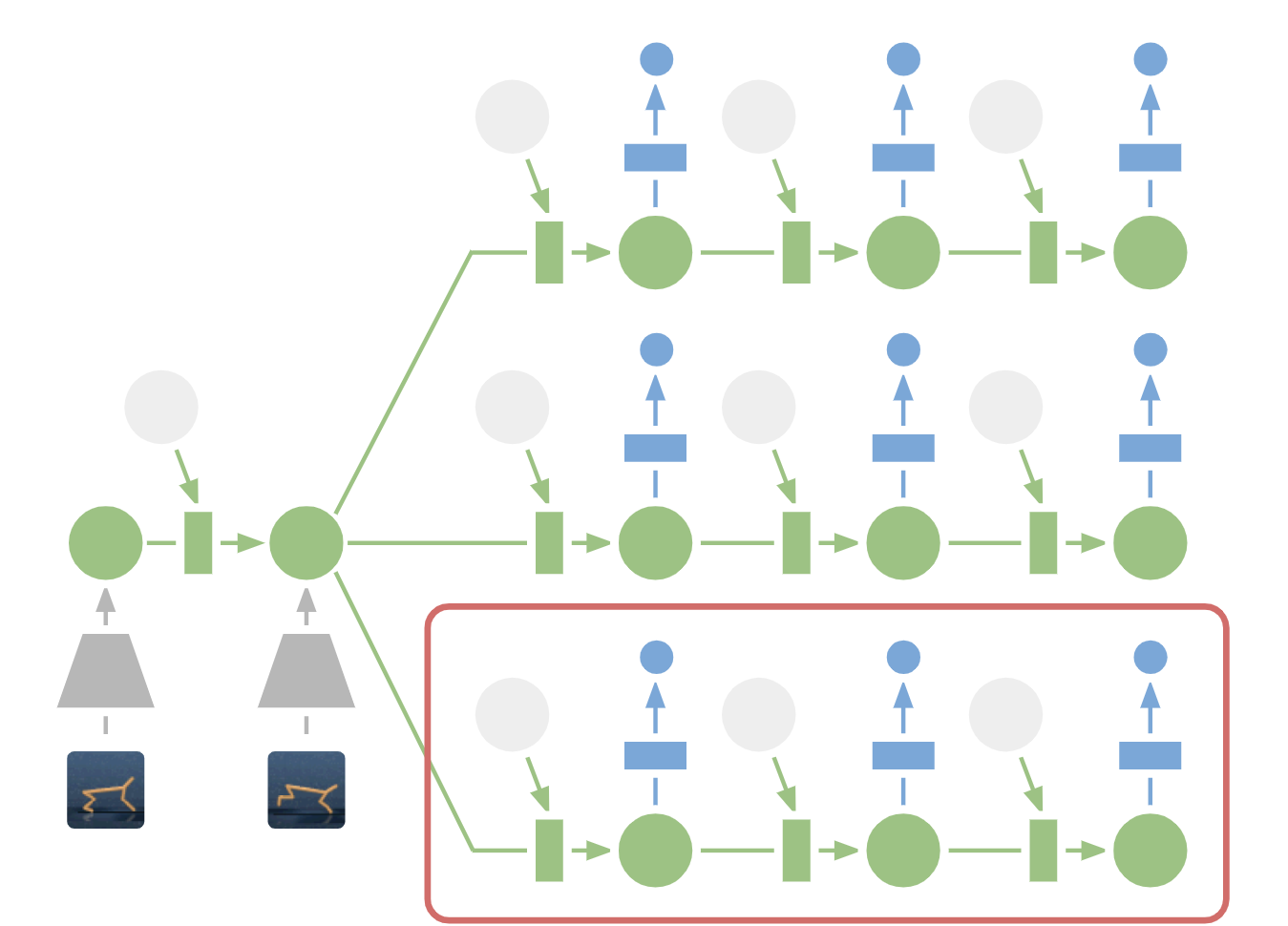
In short, PlaNet learns a dynamics model given image inputs and efficiently plans with it to gather new experience. In contrast to previous methods that plan over images, we rely on a compact sequence of hidden or latent states. This is called a latent dynamics model: instead of directly predicting from one image to the next image, we predict the latent state forward. The image and reward at each step is then generated from the corresponding latent state. By compressing the images in this way, the agent can automatically learn more abstract representations, such as positions and velocities of objects, making it easier to predict forward without having to generate images along the way.

Learned Latent Dynamics Model: In a latent dynamics model, the information of the input images is integrated into the hidden states (green) using the encoder network (grey trapezoids). The hidden state is then projected forward in time to predict future images (blue trapezoids) and rewards (blue rectangle).

To learn an accurate latent dynamics model, we introduce:

  • A Recurrent State Space Model: A latent dynamics model with both deterministic and stochastic components, allowing to predict a variety of possible futures as needed for robust planning, while remembering information over many time steps. Our experiments indicate both components to be crucial for high planning performance.
  • A Latent Overshooting Objective: We generalize the standard training objective for latent dynamics models to train multi-step predictions, by enforcing consistency between one-step and multi-step predictions in latent space. This yields a fast and effective objective that improves long-term predictions and is compatible with any latent sequence model.

While predicting future images allows us teach the model, encoding and decoding images (trapezoids in the figure above) requires significant computation, which would slow down planning. However, planning in the compact latent state space is fast since we only need to predict future rewards, and not images, to evaluate an action sequence. For example, the agent can imagine how the position of a ball and its distance to the goal will change for certain actions, without having to visualize the scenario. This allows us to compare 10,000 imagined action sequences with a large batch size every time the agent chooses an action. We then execute the first action of the best sequence found and replan at the next step.

Planning in Latent Space: For planning, we encode past images (gray trapezoid) into the current hidden state (green). From there, we efficiently predict future rewards for multiple action sequences. Note how the expensive image decoder (blue trapezoid) from the previous figure is gone. We then execute the first action of the best sequence found (red box).

Compared to our preceding work on world models, PlaNet works without a policy network — it chooses actions purely by planning, so it benefits from model improvements on the spot. For the technical details, check out our online research paper or the PDF version.

PlaNet vs. Model-Free Methods
We evaluate PlaNet on continuous control tasks. The agent is only given image observations and rewards. We consider tasks that pose a variety of different challenges:

  • A cartpole swing-up task, with a fixed camera, so the cart can move out of sight. The agent thus must absorb and remember information over multiple frames.
  • A finger spin task that requires predicting two separate objects, as well as the interactions between them.
  • A cheetah running task that includes contacts with the ground that are difficult to predict precisely, calling for a model that can predict multiple possible futures.
  • A cup task, which only provides a sparse reward signal once a ball is caught. This demands accurate predictions far into the future to plan a precise sequence of actions.
  • A walker task, in which a simulated robot starts off by lying on the ground, and must first learn to stand up and then walk.
PlaNet agents trained on a variety of image-based control tasks. The animation shows the input images as the agent is solving the tasks. The tasks pose different challenges: partial observability, contacts with the ground, sparse rewards for catching a ball, and controlling a challenging bipedal robot.

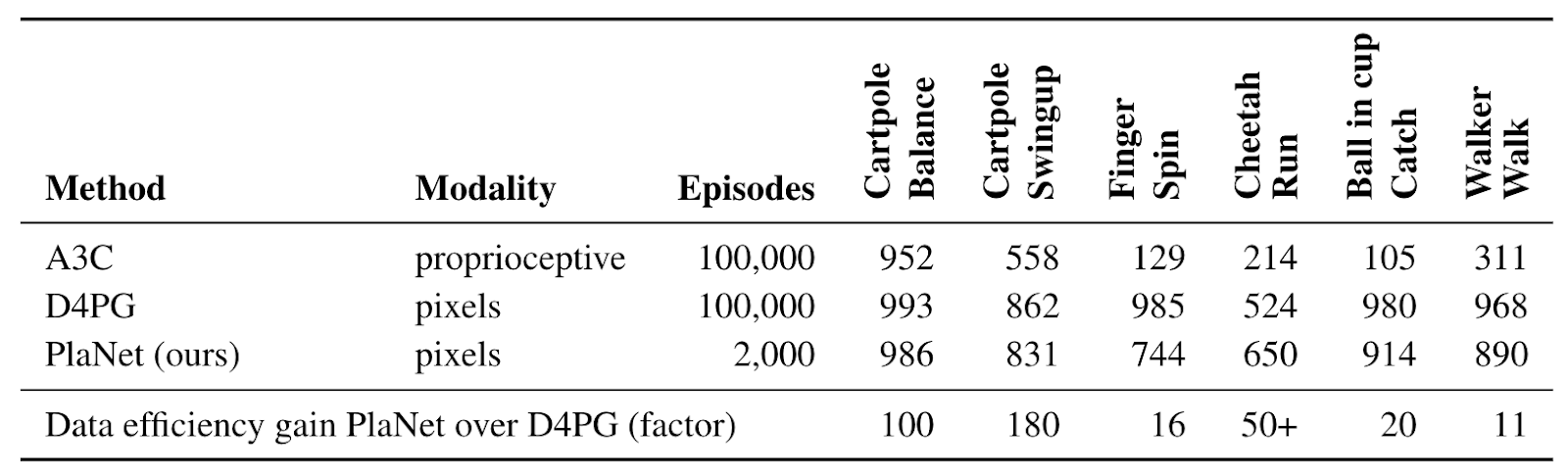
Our work constitutes one of the first examples where planning with a learned model outperforms model-free methods on image-based tasks. The table below compares PlaNet to the well-known A3C agent and the D4PG agent, that combines recent advances in model-free RL. The numbers for these baselines are taken from the DeepMind Control Suite. PlaNet clearly outperforms A3C on all tasks and reaches final performance close to D4PG while, using 5000% less interaction with the environment on average.

One Agent for All Tasks
Additionally, we train a single PlaNet agent to solve all six tasks. The agent is randomly placed into different environments without knowing the task, so it needs to infer the task from its image observations. Without changes to the hyper parameters, the multi-task agent achieves the same mean performance as individual agents. While learning slower on the cartpole tasks, it learns substantially faster and reaches a higher final performance on the challenging walker task that requires exploration.

Video predictions of the PlaNet agent trained on multiple tasks. Holdout episodes collected with the trained agent are shown above and open-loop agent hallucinations below. The agent observes the first 5 frames as context to infer the task and state and accurately predicts ahead for 50 steps given a sequence of actions.

Conclusion
Our results showcase the promise of learning dynamics models for building autonomous RL agents. We advocate for further research that focuses on learning accurate dynamics models on tasks of even higher difficulty, such as 3D environments and real-world robotics tasks. A possible ingredient for scaling up is the processing power of TPUs. We are excited about the possibilities that model-based reinforcement learning opens up, including multi-task learning, hierarchical planning and active exploration using uncertainty estimates.

Acknowledgements
This project is a collaboration with Timothy Lillicrap, Ian Fischer, Ruben Villegas, Honglak Lee, David Ha and James Davidson. We further thank everybody who commented on our paper draft and provided feedback at any point throughout the project.

Using TensorFlow eager execution with Amazon SageMaker script mode

In this blog post, I’ll discuss how to use Amazon SageMaker script mode to train models with TensorFlow’s eager execution mode. Eager execution is the future of TensorFlow; although it is available now as an option in recent versions of TensorFlow 1.x, it will become the default mode of TensorFlow 2. I’ll provide a brief overview of script mode and eager execution, and then present a typical regression task scenario. Next, I’ll describe a workflow that solves this task using script mode and eager execution together. The notebook and related code for this blog post is available on GitHub. Let’s begin with a look at script mode.

Amazon SageMaker script mode

Amazon SageMaker provides APIs and prebuilt containers that make it easy to train and deploy models using several popular machine learning (ML) and deep learning frameworks such as TensorFlow. You can use Amazon SageMaker to train and deploy models using custom TensorFlow code without having to worry about building containers or managing the underlying infrastructure. The Amazon SageMaker Python SDK TensorFlow estimators, and the Amazon SageMaker open source TensorFlow container, make it easy to write a TensorFlow script and then simply run it in Amazon SageMaker. The preferred way to leverage these capabilities is to use script mode.

Amazon SageMaker script mode was launched around AWS re:Invent 2018. It replaces the previous legacy mode, which requires structuring training code around a defined interface of specific functions and the TensorFlow Estimator API. Starting with TensorFlow version 1.11, you can use script mode with Amazon SageMaker prebuilt TensorFlow containers to train TensorFlow models with the same kind of training script you would use outside SageMaker. Your script mode code does not need to comply with any specific Amazon SageMaker-defined interface or use any specific TensorFlow API.

Although a script mode training script is very similar to a training script you might use outside of Amazon SageMaker, you also can access useful properties about the Amazon SageMaker training environment through various environment variables you set. For example, these environment variables are used to specify the dataset location (local or in Amazon S3) and hyperparameters for the algorithm. As shown in the following code snippet, if your code is written in Python, typically the code that does that actual training is placed in a main guard (if __name__ == “__main__”) since Amazon SageMaker imports the script. The main guard prevents the code from being run until Amazon SageMaker is ready to do so.


if __name__ == "__main__":
        
    args, _ = parse_args()
    
    x_train, y_train = get_train_data(args.train)
    x_test, y_test = get_test_data(args.test)
    
    device = '/cpu:0' 
    print(device)
    batch_size = args.batch_size
    epochs = args.epochs
    print('batch_size = {}, epochs = {}'.format(batch_size, epochs))

    with tf.device(device):
        
        model = get_model()
        optimizer = tf.train.GradientDescentOptimizer(0.1)
        model.compile(optimizer=optimizer, loss='mse')    
        model.fit(x_train, y_train, batch_size=batch_size, epochs=epochs,
                  validation_data=(x_test, y_test))

        # evaluate on test set
        scores = model.evaluate(x_test, y_test, batch_size, verbose=2)
        print("Test MSE :", scores)

        # save checkpoint for locally loading in notebook
        saver = tfe.Saver(model.variables)
        saver.save(args.model_dir + '/weights.ckpt')
        # create a separate SavedModel for deployment to a SageMaker endpoint with TensorFlow Serving
        tf.contrib.saved_model.save_keras_model(model, args.model_dir)

In the flow of a typical script mode script, first the command line arguments are fetched, then the data is loaded, and then the model is set up. Next is the actual training, either using convenience methods supplied by tf.keras, or using a training loop that you define. Saved models should go into the /opt/ml/model directory of the container, from which they will be automatically uploaded to Amazon S3 prior to teardown of the container when training is completed.

 TensorFlow eager execution

Eager execution is the future of TensorFlow, and it’s a major paradigm shift. Recently introduced as a more intuitive and dynamic alternative to the original graph mode of TensorFlow, eager execution will become the default mode of TensorFlow 2.

The interface of eager execution is imperative:  Operations are executed immediately, rather than being used to build a static computational graph. Advantages of eager execution include a more intuitive interface with natural control flow and less boilerplate, simplified debugging, and support for dynamic models and almost all of the available TensorFlow operations. Another key difference between eager execution and graph mode is that for graph mode, program state such as variables is globally stored, and a state object’s lifetime is managed by a tf.Session object. By contrast, for eager execution the lifetime of state objects is determined by the lifetime of their corresponding Python objects. This makes it easier to reason about how your code will work, as well as debug it.

In addition to these advantages, eager execution also works with the tf.keras API to make rapid prototyping even easier. If tf.keras is used, the model can be built using the tf.keras functional API or using a subclass from tf.Keras.Model. After model setup with tf.keras, you can simply compile it, call the fit method to train, evaluate on a test set, and save the model. If you’re not using tf.keras, you define your own training loop, and use tf.GradientTape to record operations for later automatic differentiation. Whether you use tf.keras or not, you can now use eager execution with Amazon SageMaker’s prebuilt TensorFlow containers, which was not possible with legacy mode but is now enabled by script mode.

 Workflow initial steps:  Data preprocessing and local mode

To demonstrate how eager execution works with script mode, we’ll focus on presenting a relatively complete workflow within Amazon SageMaker. The workflow includes local and hosted training, as well as inference, in the context of a straightforward regression task. The task involves predicting house prices based on the well-known, public Boston Housing dataset. This dataset contains 13 features that apply to the housing stock of towns in the Boston area, including average number of rooms, accessibility to radial highways, adjacency to the Charles River, etc. To follow along with this blog post, we recommend that you set up an Amazon SageMaker notebook instance. If you don’t have one already see the Amazon SageMaker Developer Guide for instructions. You can upload the notebook and related code from the GitHub repository for this blog post.

After preprocessing the data and writing a training script, the next step is to make sure your code is working as expected. For example, you might train the model for only a few epochs, or train the model on only small sample of the dataset rather than the full dataset. A convenient way to do this is to use Amazon SageMaker local mode training. To train in local mode, it is necessary to have Docker Compose or NVIDIA-Docker-Compose (for GPU) installed in the notebook instance. The example code has a setup shell script you can run to check this and install missing software, if any.

The following code snippet shows how to set up a TensorFlow Estimator and then starts a training job for only a few epochs to confirm that the code is working. One of the key parameters for an Estimator is the train_instance_type, which is the kind of hardware on which the training will run. In the case of local mode, we simply set this parameter to ‘local’ to invoke local mode training on the CPU, or to ‘local_gpu’ if the instance has a GPU. Other parameters of note are the algorithm’s hyperparameters, which are passed in as a dictionary, and a Boolean parameter, which indicates that we are using script mode.

import sagemaker
from sagemaker.tensorflow import TensorFlow

model_dir = '/opt/ml/model'
train_instance_type = 'local'
hyperparameters = {'epochs': 10, 'batch_size': 128}
local_estimator = TensorFlow(entry_point='train.py',
                       model_dir=model_dir,
                       train_instance_type=train_instance_type,
                       train_instance_count=1,
                       hyperparameters=hyperparameters,
                       role=sagemaker.get_execution_role(),
                       base_job_name='tf-eager-scriptmode-bostonhousing',
                       framework_version='1.12.0',
                       py_version='py3',
                       script_mode=True)

inputs = {'train': f'file://{train_dir}',
          'test': f'file://{test_dir}'}

local_estimator.fit(inputs)

To start a training job, we call local_estimator.fit(inputs), where inputs is a dictionary where the keys and named channels have values pointing to the dataset’s location. The local_estimator.fit(inputs) invocation downloads locally to the notebook instance a prebuilt TensorFlow container with TensorFlow for Python 3, CPU version. It then simulates an Amazon SageMaker training job. When training starts, the TensorFlow container executes the train.py script, passing hyperparameters as command line script arguments. You can confirm that the script is working by viewing the logs that are output in the notebook cell, including metrics for each epoch of training.

After we’ve confirmed with local mode that the code is working, we also have a model checkpoint saved in Amazon S3 that we can retrieve and load anywhere, including our notebook instance. As a further sanity check, we can then use the model to make predictions and compare them with the test set. If you do so for the Boston Housing dataset, keep in mind that the housing values are in units of $1000s. (In case you’re wondering why the actual values seem relatively low compared to today’s big city housing prices: the paper referencing the dataset was originally published in 1978.) After we confirm that our code is working, let’s move on to hosted training.

Hosted training in Amazon SageMaker

Hosted training is preferred for doing complete training on the full dataset, especially for large-scale, distributed training. When we did the local mode training, the data was accessed from local directories. Keep in mind that Amazon S3 also can be used to hold training data for local mode if you would prefer to keep all of your data in one place. However, before starting hosted training, the data must be uploaded to an Amazon S3 bucket, as shown in the notebook.

After uploading the data, we’re ready to set up an Amazon SageMaker Estimator object. It is similar to the local mode Estimator, except (1) the train_instance_type has been set to a specific instance type instead of ‘local’ for local mode, and (2) the inputs argument to the fit invocation are set to Amazon S3 locations. Also, since we’re ready to do full-scale training, the number of epochs has been increased. With these changes, we simply call the fit method again to start the actual hosted training.

train_instance_type = 'ml.c4.xlarge'
hyperparameters = {'epochs': 30, 'batch_size': 128}

estimator = TensorFlow(entry_point='train.py',
                       model_dir=model_dir,
                       train_instance_type=train_instance_type,
                       train_instance_count=1,
                       hyperparameters=hyperparameters,
                       role=sagemaker.get_execution_role(),
                       base_job_name='tf-eager-scriptmode-bostonhousing',
                       framework_version='1.12.0',
                       py_version='py3',
                       script_mode=True)

estimator.fit(inputs)

predictor = estimator.deploy(initial_instance_count=1,instance_type='ml.m4.xlarge')
results = predictor.predict(x_test[:10])['predictions'] 

As with local mode training, hosted training produces a model saved in Amazon S3 that we can retrieve and load. We can then make predictions and compare them with the test set. This also demonstrates the modularity of Amazon SageMaker. Having trained the model in Amazon SageMaker, you can now take the model out of Amazon SageMaker and run it anywhere.

Alternatively, you can deploy the model using the Amazon SageMaker hosted endpoints functionality. To do so with TensorFlow, the model must be saved in the TensorFlow SavedModel format rather than a model checkpoint format, as required by TensorFlow Serving. As shown in the last code snippet above, deployment to a hosted endpoint is simply accomplished with one line of code by calling the Estimator’s deploy method.

Conclusion

One of the goals of Amazon SageMaker is to enable data scientists and developers to quickly and easily build, train, and deploy ML models. When script mode is combined with TensorFlow eager execution mode, it’s easy to set up a workflow for rapid prototyping to large-scale training and deployment you can use for a wide variety of data science projects. If you prefer the TensorFlow original static computational graph mode, you also can use script mode. It’s your choice, and it’s just one of the many flexible options provided by Amazon SageMaker.


About the Author

Brent Rabowsky focuses on data science at AWS, and leverages his expertise to help AWS customers with their own data science projects.


Controlling False Discoveries in Large-Scale Experimentation: Challenges and Solutions

“Scientific research has changed the world. Now it needs to change itself.”

– The Economist, 2013

There has been a growing concern about the validity of scientific findings. A multitude of journals, papers and reports have recognized the ever smaller number of replicable scientific studies. In 2016, one of the giants of scientific publishing, Nature, surveyed about 1,500 researchers across many different disciplines, asking for their stand on the status of reproducibility in their area of research. One of the many takeaways to the worrisome results of this survey is the following: 90% of the respondents agreed that there is a reproducibility crisis, and the overall top answer to boosting reproducibility was “better understanding of statistics”. Indeed, many factors contributing to the explosion of irreproducible research stem from the neglect of the fact that statistics is no longer as static as it was in the first half of the 20th century, when statistical hypothesis testing came into prominence as a theoretically rigorous proposal for making valid discoveries with high confidence.

Continue reading

Read WordPress sites through Amazon Alexa devices

At the beginning of last year we announced an Amazon Polly plugin for WordPress. This plugin allows blog and website creators who are using WordPress to quickly and easily create audio versions of their posts, articles and websites. A few months later, we updated the plugin with the ability to quickly translate the content of websites to other languages using the Amazon Translate service. This functionality, together with the ability to create audio versions, allows you to voice the content of sites in translated languages. We want to allow creators and authors to reach more readers/listeners around the world using the latest AI services offered by AWS. Today we are happy to announce another extension of the plugin, which allows you to extend WordPress websites and blogs through Alexa devices. This opens new possibilities for the creators and authors of websites to reach an even broader audience. It also makes it easier for people to listen to their favorite blogs by just asking Alexa to read them! So let’s dive deep, and I’ll show you how to integrate your WordPress website with Alexa.

In addition, today we’re announcing that the official name for the plugin is changing to Amazon AI Plugin for WordPress to better reflect the broad integration with the AWS AI ecosystem.

The following diagram presents the flow of interactions and components that are required to expose your website through Alexa.

Let’s step through the process that we are going to implement:

  1. The user invokes a new Alexa skill, for example by saying: Alexa, ask Demo Blog for the latest update.
    1. The skill itself is created using one of the Alexa Skill Blueprints. This allows you to expose your skill through Alexa devices even if you don’t have deep technical knowledge.
  2. The Alexa skill analyzes the call and RSS feed that was generated by the Amazon AI plugin for WordPress, and then returns the link to the audio version of the latest article.
  3. Based on the link provided by the feed, Alexa reads the article by playing the audio file saved on Amazon S3.

The diagram illustrates that AWS services, such as Amazon Polly and Amazon Translate, are used by the WordPress plugin to generate audio versions.

So let’s go into details, and let’s expose our site using Alexa! We won’t be describing the process of installing the plugin on your WordPress website in this blog post. You can read about it in this post, or follow the instructions that are provided on the WordPress plugin website. In general, it should take just around 15 minutes to do this phase. Remember that after enabling the plugin, you should enable the text-to-speech functionality and Amazon Pollycast functionality – which will then generate an RSS feed on your WordPress site which we will be consuming in next phase. Enable Amazon S3 as the default storage for your files. It’s important that your website uses a secure HTTPS connection to expose its feed to Alexa.

After completing these steps, you should note the Amazon Pollycast link that is displayed on the podcast tab of the plugin.

If you open the feed link you should be able to see information about the posts you have published.

The next step is to create an actual skill. As I have already mentioned before, it will be really easy, because we will be using existing Alexa Skill Blueprints. Open the Alexa Skill Blueprints page, and look for the Blog blueprint.

After you find it, choose Make Your Own. After this a three-step wizard opens, which will allow you to create your skill. On the first page provide the link to your RSS feed that you have copied before, and then choose Next: Experience.

Next, you could customize your skill. For this blog post, we’ll leave it as it is, and choose Next: Name.

The next step is choosing the right name for your skill. This is the name that will be used by your readers/listeners to activate the skill and ask Alexa to read a new article. In my example I will use the name Demo Blog. Next, choose Next: Create Skill.

It will take a couple of minutes for the skill to be created, you can grab a quick coffee meanwhile.

Now, when you click the Skills you’ve made link on the top of the page, you should see your own Alexa Skill. Congratulations!

The following short video presents what the solution should look like:

Conclusion

At this stage, your skill is only available from devices that are registered on the Amazon account which you have used to build your skill. The next step would be to publish it as an official skill on the skill store. To do this, open the details page of your skill, where you will find a Publish to  Skill Store button. Just follow those instructions.

You can review the process of publishing the skill in this video:

When you are finished, you’ll be able to announce the world that your website is available on Alexa! Congratulations!


About the Author

Tomasz Stachlewski is a Solutions Architect at AWS, where he helps companies of all sizes (from startups to enterprises) in their cloud journey. He is a big believer in innovative technology, such as serverless architecture, which allows companies to accelerate their digital transformation.

Gubagoo uses Amazon Translate to build translated live chat for automotive dealers

Gubagoo is the leading provider of advanced communication solutions for automotive dealers. Gubagoo understands that automotive customers want a personalized experience and helpful information whenever they purchase a car or book a service appointment. In addition, customers want to be communicated with in their native language. However, dealerships in the US have a difficult time crafting these communications since their staff typically speaks English only. To address this problem, Gubagoo offers a live chat solution called ChatSmart. A dealership can integrate ChatSmart with its website to manage initial customer conversations in multiple languages in real-time. To accomplish this ChatSmart uses Amazon Translate, a neural machine translation service that delivers fast, high-quality, and affordable language translations.

The ChatSmart solution looks like this:

As more dealerships adopted ChatSmart, Gubagoo realized that more than 10 percent of conversations were in a language other than English. “By giving car shoppers the ability to communicate in their language of choice, we are able to reach more consumers and generate more leads for dealers,” said Ilia Alshanetsky, CTO of Gubagoo. “We realized that the most efficient way to do so is by seamlessly integrating our solution to a neural machine translation services provider.” Gubagoo tested a few different machine translation services and chose Amazon Translate because it consistently provided translation two times faster at 25 percent less cost than other solutions.

“With Amazon Translate, we can now successfully serve dealerships that sell to non-English speaking consumers,” continued Alshanetsky. “For example, we serve our dealership clients in Puerto Rico by managing any conversations initiated by Spanish speaking customers using Amazon Translate, of which 48 percent have converted into leads. The translation is so natural that it is difficult for consumers to tell that they are chatting with a non-Spanish speaker.”

When a customer initiates a conversation using the live chat, the Amazon Comprehend Language Detection API recognizes the language used by the customer. When texts are in English, no translations are required. If these texts are in a language other than English, the Amazon Translate API will translate the texts into English and deliver them to the chat specialist. When the chat specialist types back in English, the Translate API will translate these responses and provide the texts in customer’s preferred language.

Here is an illustration of this workflow:

Example: ChatSmart and Amazon Translate work together

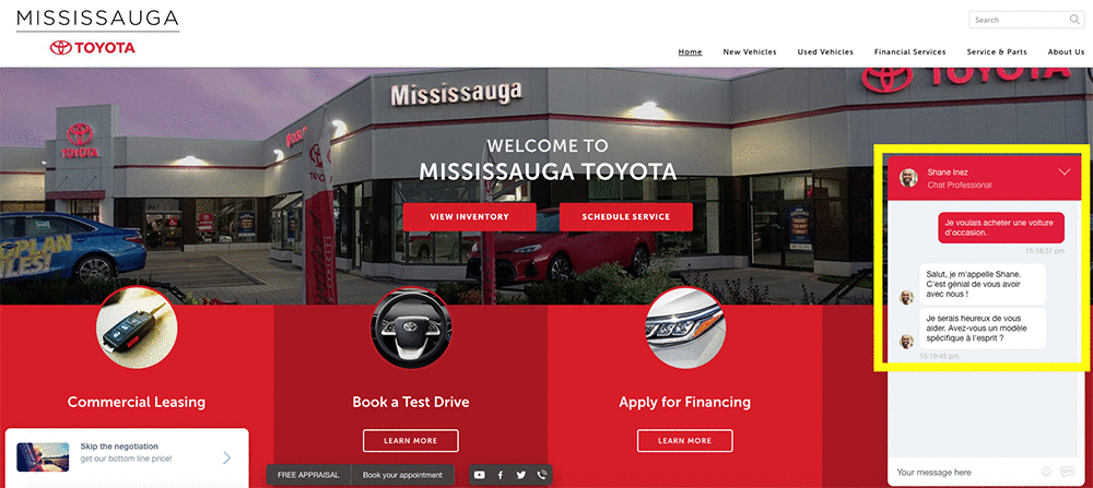
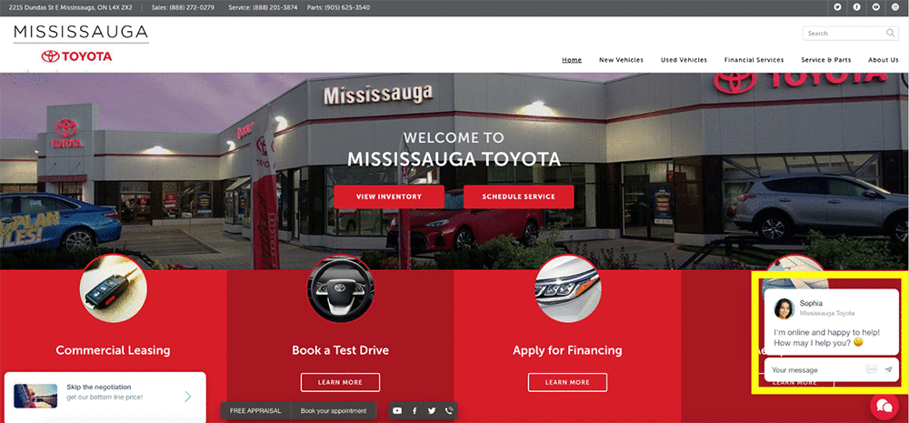
For example, here is how the family-owned-and-operated Mississauga Toyota dealership is using ChatSmart integrated with Amazon Translate. As soon as I enter their online site, I’m greeted by Sophia. See the bottom-right corner of the following screenshot.

I decided to ask, “I want to buy a used car” in French. Within a few seconds, I got two replies back in French from Shane! See Shane’s responses in the bottom-right corner of the following screenshot.

  • “Salut, je m’appelle Shane. C’est génial de vous avoir avec nous!”, which means Hi, my name is Shane. It’s great to have you with us!” in English.
  • “Je serais heureux de vous aider. Avez-vous un modèle spécifique à l’esprit?”, which means, I would be happy to help you. Do you have a specific model in mind?” in English.

“To us the ROI is clear. The amount we spend on Amazon Translate is recouped many times over in terms of the revenue and flexibility we can offer to our customers,” stated Alshanetsky. “This is also just the beginning. Amazon Translate is opening the door to new business opportunities both locally and abroad allowing us to connect with a wider range of customers, which are in some cases underserved.”


About the Author

Woo Kim is a Product Marketing Manager for AWS machine learning services. He spent his childhood in South Korea and now lives in Seattle, WA. In his spare time, he enjoys playing volleyball and tennis.



Using Global Localization to Improve Navigation

One of the consistent challenges when navigating with Google Maps is figuring out the right direction to go: sure, the app tells you to go north – but many times you’re left wondering, “Where exactly am I, and which way is north?” Over the years, we’ve attempted to improve the accuracy of the blue dot with tools like GPS and compass, but found that both have physical limitations that make solving this challenge difficult, especially in urban environments.

We’re experimenting with a way to solve this problem using a technique we call global localization, which combines Visual Positioning Service (VPS), Street View, and machine learning to more accurately identify position and orientation. Using the smartphone camera as a sensor, this technology enables a more powerful and intuitive way to help people quickly determine which way to go.

Due to limitations with accuracy and orientation, guidance via GPS alone is limited in urban environments. Using VPS, Street View and machine learning, Global Localization can provide better context on where you are relative to where you’re going.

In this post, we’ll discuss some of the limitations of navigation in urban environments and how global localization can help overcome them.

Where GPS Falls Short
The process of identifying the position and orientation of a device relative to some reference point is referred to as localization. Various techniques approach localization in different ways. GPS relies on measuring the delay of radio signals from multiple dedicated satellites to determine a precise location. However, in dense urban environments like New York or San Francisco, it can be incredibly hard to pinpoint a geographic location due to low visibility to the sky and signals reflecting off of buildings. This can result in highly inaccurate placements on the map, meaning that your location could appear on the wrong side of the street, or even a few blocks away.

GPS signals bouncing off facades in an urban environment.

GPS has another technical shortcoming: it can only determine the location of the device, not the orientation. Sometimes, sensors in your mobile device can remedy the situation by measuring the magnetic and gravity field of the earth and the relative motion of the device in order to give rough estimates of your orientation. But these sensors are easily skewed by magnetic objects such as cars, pipes, buildings, and even electrical wires inside the phone, resulting in errors that can be inaccurate by up to 180 degrees.

A New Approach to Localization
To improve the precision position and orientation of the blue dot on the map, a new complementary technology is necessary. When walking down the street, you orient yourself by comparing what you see with what you expect to see. Global localization uses a combination of techniques that enable the camera on your mobile device to orient itself much as you would.

VPS determines the location of a device based on imagery rather than GPS signals. VPS first creates a map by taking a series of images which have a known location and analyzing them for key visual features, such as the outline of buildings or bridges, to create a large scale and fast searchable index of those visual features. To localize the device, VPS compares the features in imagery from the phone to those in the VPS index. However, the accuracy of localization through VPS is greatly affected by the quality of the both the imagery and the location associated with it. And that poses another question—where does one find an extensive source of high-quality global imagery?

Enter Street View
Over 10 years ago we launched Street View in Google Maps in order to help people explore the world more deeply. In that time, Street View has continued to expand its coverage of the world, empowering people to not only preview their route, but also step inside famous landmarks and museums, no matter where they are. To deliver global localization with VPS, we connected it with Street View data, making use of information gathered and tested from over 93 countries across the globe. This rich dataset provides trillions of strong reference points to apply triangulation, helping more accurately determine the position of a device and guide people towards their destination.

Features matched from multiple images.

Although this approach works well in theory, making it work well in practice is a challenge. The problem is that the imagery from the phone at the time of localization may differ from what the scene looked like when the Street View imagery was collected, perhaps months earlier. For example, trees have lots of rich detail, but change as the seasons change and even as the wind blows. To get a good match, we need to filter out temporary parts of the scene and focus on permanent structure that doesn’t change over time. That’s why a core ingredient in this new approach is applying machine learning to automatically decide which features to pay attention to, prioritizing features that are likely to be permanent parts of the scene and ignoring things like trees, dynamic light movement, and construction that are likely transient. This is just one of the many ways in which we use machine learning to improve accuracy.

Combining Global Localization with Augmented Reality
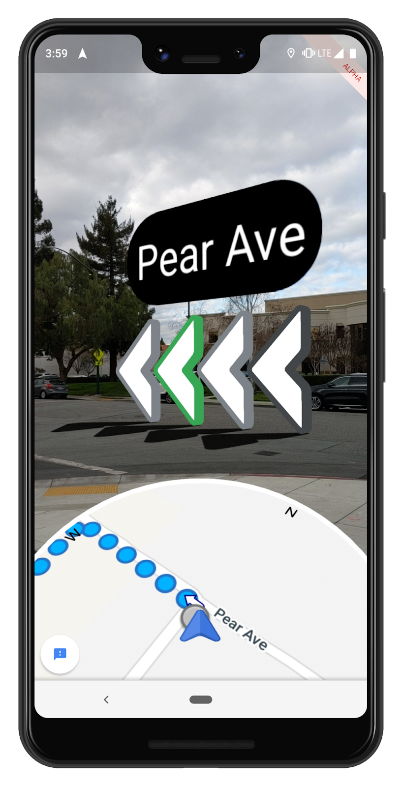
Global localization is an additional option that users can enable when they most need accuracy. And, this increased precision has enabled the possibility of a number of new experiences. One of the newest features we’re testing is the ability to use ARCore, Google’s platform for building augmented reality experiences, to overlay directions right on top of Google Maps when someone is in walking navigation mode. With this feature, a quick glance at your phone shows you exactly which direction you need to go.

Although early results are promising, there’s significant work to be done. One outstanding challenge is making this technology work everywhere, in all types of conditions—think late at night, in a snowstorm, or in torrential downpour. To make sure we’re building something that’s truly useful, we’re starting to test this feature with select Local Guides, a small group of Google Maps enthusiasts around the world who we know will offer us the feedback about how this approach can be most helpful.

Like other AI-driven camera experiences such as Google Lens (which uses the camera to let you search what you see), we believe the ability to overlay directions over the real world environment offers an exciting and useful way to use the technology that already exists in your pocket. We look forward to continuing to develop this technology, and the potential for smartphone cameras to add new types of valuable experiences.