Even in today’s highly digital workplace, documents are often manually processed in many enterprise workflows, including workflows in financial services. Alkymi, founded by a team from Bloomberg and x.ai, enlists automation to streamline this laborious and error-prone work. Using deep learning models hosted on Amazon SageMaker, Alkymi identifies patterns and relationships in unstructured data and synthesizes documents into actionable data. This gives enterprises the potential to save billions in the process by removing a stubborn barrier to automation.
Alkymi uses AWS as their primary AI/ML platform. The CEO of Alkymi, Harald Collet, notes, “We apply AI to help automate tasks on documents that require human comprehension, and AWS has enabled us to quickly launch new functionality with the security and scalability that financial services customers require.” As Alkymi ingests documents, emails, and images, the platform automates data extraction and data entry tasks by using various AWS services. “AWS allows us to scale our platform to handle customers of all sizes. Amazon SageMaker has improved our development process by providing our data scientists with a way to train and deploy models to production,” remarks Alkymi CTO Steven She.
Alkymi’s data pipeline begins with ingesting documents and images through their REST API hosted on Amazon Elastic Container Service (ECS) or as email received through Amazon Simple Email Service (SES). The data are saved into encrypted Amazon S3 buckets based in geo-regions that adhere to the compliance policies of our customers.
Documents are placed into messaging queues, then processed by pipelines of Amazon SageMaker machine learning and natural language processing models. The data science team loves Amazon SageMaker’s streamlined UI and workflow, which make it possible for the data scientists to train and deploy the models themselves. Alkymi’s sophisticated ML models are both trained and hosted on Amazon SageMaker. With just a few clicks, the team can identify the context of the information on each page, such as tables, paragraphs, info boxes, and charts. This ensures that the natural language processing can be maximally effective as it operates within context. All model predictions come with a confidence score. Documents where the models have a low confidence score are flagged and routed for human review.
After clients deploy Alkymi in production, end users, such as business or ops analysts, no longer need to use a manual copy-and-paste workflow. Instead, they only need to validate a small amount of exceptions that have been flagged by Alkymi. These corrections fuel a feedback loop that improves model accuracy and performance over time. As a result, the business can move forward quicker, with fewer missed opportunities, less risk, and much less operational overhead. Alkymi’s customers estimate that the platform automates up to 90 percent of manual document processing tasks and cuts errors by 50 percent—all while generating actionable insights in real time rather than days or weeks later.
For Alkymi, the business impact is exciting, and the potential is limitless. As customers are rapidly embracing AI / ML technologies, Alkymi is committed to maintaining its position as a pioneer in a fast-growing market. Harald Collet comments, “We’re tackling a massive opportunity to help financial services companies transform how works get done and rapidly innovate to keep pace with the market.” Building on the AWS platform and energized by the support of the AWS Accelerate program, Alkymi is on an unstoppable mission to deliver digital transformation for financial services.
About the Author
Marisa Messina is on the AWS AI marketing team, where her job includes identifying the most innovative AWS-using customers and showcasing their inspiring stories. Prior to AWS, she worked on consumer-facing hardware and then university-facing cloud offerings at Microsoft. Outside of work, she enjoys exploring the Pacific Northwest hiking trails, cooking without recipes, and dancing in the rain.
Posted by Christine Kaeser-Chen, Software Engineer and Serge Belongie, Visiting Faculty, Google AI
In recent years, fine-grained visual recognition competitions (FGVCs), such as the iNaturalist species classification challenge and the iMaterialist product attribute recognition challenge, have spurred progress in the development of image classification models focused on detection of fine-grained visual details in both natural and man-made objects. Whereas traditional image classification competitions focus on distinguishing generic categories (e.g., car vs. butterfly), the FGVCs go beyond entry level categories to focus on subtle differences in object parts and attributes. For example, rather than pursuing methods that can distinguish categories, such as “bird”, we are interested in identifying subcategories such as “indigo bunting” or “lazuli bunting.”
Previous challenges attracted a large number of talented participants who developed innovative new models for image recognition, with morethan500 teams competing at FGVC5 at CVPR 2018. FGVC challenges have also inspired new methods such as domain-specific transfer learning and estimating test-time priors, which have helped fine-grained recognition tasks reach state-of-the-art performance on several benchmarking datasets.
In order to further spur progress in FGVC research, we are proud to sponsor and co-organize the 6th annual workshop on Fine-Grained Visual Categorization (FGVC6), to be held on June 17th in Long Beach, CA at CVPR 2019. This workshop brings together experts in computer vision with specialists focusing on biodiversity, botany, fashion, and the arts, to address the challenges of applying fine-grained visual categorization to real-life settings.
The FGVC workshop at CVPR focuses on subordinate categories, including (from left to right, top to bottom) animal species from wildlife camera traps, retail products, fashion attributes, cassava leaf disease, Melastomataceae species from herbarium sheets, animal species from citizen science photos, butterfly and moth species, cuisine of dishes, and fine-grained attributes for museum art objects.
In the iMet Collection challenge, participants compete to train models on artistic attributes including object presence, culture, content, theme, and geographic origin. The Metropolitan Museum of Art provided a large training dataset for this task based on subject matter experts’ descriptions of their museum collections. This dataset highlights the challenge of inferring fine-grained attributes that are grounded in the visual context indirectly (e.g., period, culture, medium).
A diverse sample of images included in the iMet Collection challenge dataset. Images were taken from the Metropolitan Museum of Art’s public domain dataset.
The iMet Collection challenge is also noteworthy for its status as the first image-based Kernels-only competition, a recently introduced option on Kaggle that levels the playing field for data scientists who might not otherwise have access to adequate computational resources. Kernel competitions provide all participants with the same hardware allowances, giving rise to a more balanced competition. Moreover, the winning models tend to be simpler than their counterparts in other competitions, since the participants must work within the compute constraints imposed by the Kernels platform.At the time of writing, the iMet Collection challenge has over 250 participating teams.
In the Herbarium challenge, researchers are invited to tackle the problem of classifying species from the flowering plant family Melastomataceae. This challenge is distinguished from the iNaturalist competition, since the included images depict dried specimens preserved on herbarium sheets, exclusively. Herbarium sheets are essential to plant science, as they not only preserve the key details of the plants for identification and DNA analysis, but also provide a rare perspective into plant ecology in a historical context. As the world’s second largest herbarium, NYBG’s Steere Herbarium collection contributed a dataset of over 46,000 specimens for this year’s challenge.
In the Herbarium challenge, participants will identify species from the flowering plant family Melastomataceae. The New York Botanical Garden (NYBG) provided a dataset of over 46,000 herbarium specimens including over 680 species. Images used with permission of the NYBG.
Every one of this year’s challenges requires deep engagement with subject matter experts, in addition to institutional coordination. By teeing up image recognition challenges in a standard format, the FGVC workshop paves the way for technology transfer from the top of the Kaggle leaderboards into the hands of everyday users via mobile apps such as Seek by iNaturalist and Merlin Bird ID. We anticipate the techniques developed by our competition participants will not only push the frontier of fine-grained recognition, but also be beneficial for applying machine vision to advance scientific exploration and curatorial studies.
Invitation to Participate We invite teams to participate in these competitions to help advance the state-of-the-art in fine-grained image recognition. Deadlines for entry into the competitions range from May 26 to June 3, depending on the challenge. The results of these competitions will be presented at the FGVC6 workshop at CVPR 2019, and will provide broad exposure to the top performing teams. We are excited to encourage the community’s development of more accurate and broadly impactful algorithms in the field of fine-grained visual categorization!
Acknowledgements We’d like to thank our colleagues and friends on the FGVC6 organizing committee for working together to advance this important area. At Google we would like to thank Hartwig Adam, Chenyang Zhang, Yulong Liu, Kiat Chuan Tan, Mikhail Sirotenko, Denis Brulé, Cédric Deltheil, Timnit Gebru, Ernest Mwebaze, Weijun Wang, Grace Chu, Jack Sim, Andrew Howard, R.V. Guha, Srikanth Belwadi, Tanya Birch, Katherine Chou, Maggie Demkin, Elizabeth Park, and Will Cukierski.
The new release of MXNet 1.4 for Amazon Elastic Inference now includes Java and Scala support. Apache MXNet is an open source deep learning framework used to build, train, and deploy deep neural networks. Amazon Elastic Inference (EI) is a service that allows you to attach low-cost GPU-powered acceleration to Amazon EC2 and Amazon SageMaker instances. Amazon EI reduces the cost of running deep learning inference by up to 75%. In this post, we will show you how to run inference in Java using MXNet and an Elastic Inference Accelerator (EIA).
Setting up Amazon Elastic Inference with Amazon EC2
Starting up an EC2 instance with an attached Amazon EI accelerator requires some pre-configuration steps when you set up your AWS account. You can use the setup tool to easily start up everything you need. Or, you can launch an instance with an accelerator by following the instructions in the Amazon Elastic Inference documentation. Here, we start with a basic Ubuntu Amazon Machine Image (AMI), and configure it for our needs. Start by connecting to your instance via SSH and installing the following dependencies:
Start by downloading and unzipping the demo project.
wget https://s3.amazonaws.com/aws-ml-blog/artifacts/inference-blog/eiaBlogPostDemo.zip
unzip eiaBlogPostDemo.zip
cd eiaBlogpostDemo
Inside the archive is a pom.xml file that will build the project with the Amazon EI MXNet dependency. It uses an additional Maven repository located on Amazon S3 that contains the Amazon EI MXNet package:
With these changes, Maven can access the appropriate repository and will automatically download the Amazon EI MXNet jar to make it accessible from the project.
Creating a ResNet-152 application
In this section we will walk through the demo code in the archive at:
src/main/java/mxnet/ImageClassificationDemo.java
Let’s write some code to perform a simple image classification using the ResNet-152 model. First, we need to download the model, names of the different image classification labels, and a test image.
String urlPath = "http://data.mxnet.io/models/imagenet";
String filePath = System.getProperty("java.io.tmpdir");

// Download Model and Image
FileUtils.copyURLToFile(new URL(urlPath + "/resnet/152-layers/resnet-152-0000.params"),
        new File(filePath, "resnet-152/resnet-152-0000.params"));
FileUtils.copyURLToFile(new URL(urlPath + "/resnet/152-layers/resnet-152-symbol.json"),
        new File(filePath, "resnet-152/resnet-152-symbol.json"));
FileUtils.copyURLToFile(new URL(urlPath + "/synset.txt"),
        new File(filePath, "resnet-152/synset.txt"));
FileUtils.copyURLToFile(new URL("https://github.com/dmlc/web-data/blob/master/mxnet/doc/tutorials/python/predict_image/cat.jpg?raw=true"),
        new File(filePath, "cat.jpg"));
Then, we create a Predictor object to run the model. It takes in an image as a 1 element batch of images where each image is a 3 x 224 x 224 NDArray of Floats. Since the image is the only input to the model, we make a list with that inputDescriptor as the only element. We also provide the path to the model on the local file system. In order to run this predictor with Amazon EI we pass in Context.eia(). You could also use Context.cpu() to run inference locally on the CPU only (this could be useful for debugging).
Now that we have the predictor, we need to get the image to run the prediction on. There are some utilities within the ObjectDetector class to help simplify this process. Let’s load the image from the file, reshape it to 224 x 224, and convert it into an NDArray.
Let’s print out the top 5 predicted classes of the image. After we execute the prediction, we need to find the results with largest confidence values. Then, we need to find the corresponding names for each element in the results from the synset.txt file.
List<String> synsetLines = FileUtils.readLines(new File(filePath + "/resnet-152/synset.txt"));

int[] best = IntStream.range(0, results.length)
        .boxed().sorted(Comparator.comparing(i -> -results[i]))
        .mapToInt(ele -> ele).toArray();

for (int i = 0; i < 5; i++) {
    int ind = best[i];
    System.out.println(i + ": " + synsetLines.get(ind) + " - " + best[ind]);
}
Building and running the ResNet-152 application
To build the project, simply navigate to the main directory containing the README and pom.xml and run mvn package. After it’s built, we can run the example by using mvn exec:java -Dexec.mainClass=mxnet.ImageClassificationDemo -Dexec.cleanupDaemonThreads=false.
Lets analyze the performance of the various configurations using the latency or time required to complete one inference call. Amazon EI accelerators are currently available in three sizes: eia1.medium, eia1.large, and eia1.xlarge. Each has from 1 to 4 GB of memory and from 8 to 32 TFLOPS of compute. For this example, we’ll run the resnet-152 model on P2, P3, C5.4xlarge, and C5.large EC2 instance types plus all EIA options.
Looking at the results, we can see the latencies of the standard instances are, from best to worst, 13.26ms for P3, 43.52ms for P2, and 64.91ms for C5.4xlarge. The latencies for the EIA instances fall between the best, P3, and the middle, P2, with 22.11ms for c5.large + eia1.xlarge, 26.28 for c5.large + eia1.large, and 41.7ms for c5.large + eia1.medium. However, the cost efficiencies of the standard EC2 instances range from $1.08 to $1.19 per 100,000 inferences while the Amazon EI accelerator instances have cost efficiencies from $.24 to $.37, up to a 78% savings.
Compared to running inferences on CPU instances such as the c5.4xlarge, the Amazon EI options are up to 56% faster, while being cheaper as well. They have better performance than the P2 while being up to 76% cheaper. Although the P3 instances have better latency, you can get up to 13 Amazon EI instances for the same price, which is 93% cheaper.
In summary, if your application requires the lowest latency available, you probably need to stick to the P3 instance type. But if your application allows for just slightly higher latencies, you can take advantage of Amazon EI and save up to 78% compared to the cost of P2 and P3 instances. The results for the EIA instances show that EIA provides another option in terms of raw performance between P2 and P3 instances, but with the best cost efficiency of any instance type. Refer to Appendix 1 for a detailed performance comparison between different CPU, GPU, and EIA flavors.
Conclusion
The Java/Scala support for MXNet on Amazon EI enables Java applications to add cost-effective deep learning acceleration to existing production systems. Using Amazon EI accelerators can reduce latencies by 56% compared to using just CPU while reducing the inference cost by up to 78%.
Appendix 1 – Raw performance and cost results for ResNet-152
This table provides the data collected across a number of instance types both with and without Amazon Elastic Inference. We show the times to do a single prediction (latency), the number of predictions per second (throughput), the cost of the instances, and the cost effectiveness ($/100k inferences). For example, if your main goal is to get minimal latency while keeping costs under control (e.g., you don’t want expensive GPU hosts), one of the best choices for you is to use a c5.2xlarge instance with an eia1.xlarge accelerator. If your primary goal is to minimize costs, and your latency requirements are more lenient, you can use a c5.large instance with an eia1.large accelerator. Compared to the latency-optimized case inference time would increase by ~28%, but the corresponding cost reduction would be ~50%.
Remember that these metrics are only for the Resnet-152 model. You would need to collect data on your application’s model in order to find the best options for you.
Instance Type
p50 Latency
p90 Latency
Throughput per sec
Instance Cost per hour
$/100k inferences
Notes
c5.4xlarge
62.73
64.91
15.94
$0.68
$1.19
c5.9xlarge
39.61
39.81
25.25
$1.53
$1.68
c5.large + eia1.medium
40.19
41.37
24.88
$0.22
$0.24
c5.large + eia1.large
26.28
27.15
38.05
$0.35
$0.25
Best for cost effectiveness with EI
c5.large + eia1.xlarge
22.11
23.13
45.23
$0.61
$0.37
c5.xlarge + eia1.medium
39.62
41.35
25.24
$0.30
$0.33
c5.xlarge + eia1.large
26.24
26.92
38.11
$0.43
$0.31
c5.xlarge + eia1.xlarge
21.04
21.61
47.52
$0.69
$0.40
c5.2xlarge + eia1.medium
38.8
43.24
25.78
$0.47
$0.50
c5.2xlarge + eia1.large
26.27
27.03
38.07
$0.60
$0.44
c5.2xlarge + eia1.xlarge
20.89
21.26
47.88
$0.86
$0.50
Best for latency with EI
p2.xlarge
43.23
43.52
23.13
$0.90
$1.08
p3.2xlarge
13.26
13.54
75.44
$3.06
$1.13
About the authors
Zach Kimberg is a Software Engineer with AWS Deep Learning working mainly on Apache MXNet for Java and Scala. Outside of work he enjoys reading, especially Fantasy.
Sam Skalicky is a Software Engineer with AWS Deep Learning and enjoys building heterogeneous high performance computing systems. He is an avid coffee enthusiast and avoids hiking at all costs.
Denis Davydenko is an Engineering Manager with AWS Deep Learning. He focuses on building Deep Learning tools that enable developers and scientists to build intelligent applications. In his spare time he enjoys spending time with his family, playing poker and video games.
During the past few years, the demand for machine learning specialists and engineers has soared. These two roles now rank among the top emerging jobs on LinkedIn. More recently, machine learning is being adopted by a wide range of industries, from medical diagnostic companies to finance firms and more. Udacity created the Intro to Machine Learning Nanodegree program and Machine Learning Engineer Nanodegree program in response to this demand to provide access to this growing tech field to a broader audience.
There is a growing demand for engineers who are able to integrate machine learning models into globally available production applications like voice assistants and recommendation engines. Knowing how to build machine learning models is a great starting point. But, to truly make an impact, a data scientist or developer needs to know how to take a model out of the lab and into the real world so that it can be used to make millions or billions of predictions.
“Industry demand for the latest AI skills is at an all-time high. In collaboration with Amazon, we’ve updated the Udacity Machine Learning Nanodegree program to make it possible to gain the latest machine learning deployment skills anywhere in the world on the AWS platform,” says Sebastian Thrun, Co-Founder, President, Executive Chairman of Udacity.
AWS Educate and Amazon SageMaker collaborated with Udacity to create new deployment content for the Machine Learning Engineer Nanodegree program. AWS Educate provides Udacity students with access to AWS content and AWS promotional credits. These benefits allow students to use Amazon SageMaker for assignments developed in tandem with AWS subject matter experts (SMEs). The course examines a variety of machine learning models as they are applied at-scale to real-world tasks. Students learn how to deploy both unsupervised and supervised algorithms, and apply them to tasks such as feature engineering and time-series forecasting. This content addresses questions such as:
How do you decide on the correct machine learning model for a given task?
How can you use cloud deployment tools such as Amazon SageMaker to work with data and improve your machine learning models?
Machine Learning Engineer Nanodegree program description from Udacity.com
In addition to learning about model deployment, students also learn about model serving and updating. The course now shows how to connect a deployed sentiment analysis model to a website by using an AWS API. After deploying the model, it’s updated to account for changes in the underlying text data – an especially valuable skill in industries that continuously collect data. By the end of this section, students should have the skills needed to train and deploy models to solve tasks of their own design!
Enroll today to get practical experience deploying machine learning models at-scale with an AWS Educate membership.
About the Author
Sally Revell is a Senior Manager, Product Marketing for AWS AI. She loves to work on innovative products that have the potential to impact people’s lives in a positive way. In her spare time, she loves to do yoga, horseback riding and being outdoors in the beauty of the Pacific Northwest.
Posted by Olivier Bachem, Research Scientist, Google AI Zürich
The ability to understand high-dimensional data, and to distill that knowledge into useful representations in an unsupervised manner, remains a key challenge in deep learning. One approach to solving these challenges is through disentangled representations, models that capture the independent features of a given scene in such a way that if one feature changes, the others remain unaffected. If done successfully, a machine learning system that is designed to navigate the real world, such as a self driving car or a robot, can disentangle the different factors and properties of objects and their surroundings, enabling the generalization of knowledge to previously unobserved situations. While, unsupervised disentanglement methods have already been used for curiosity driven exploration, abstract reasoning, visual concept learning and domain adaptation for reinforcement learning, recent progress in the field makes it difficult to know how well different approaches work and the extent of their limitations.
In “Challenging Common Assumptions in the Unsupervised Learning of Disentangled Representations” (to appear at ICML 2019), we perform a large-scale evaluation on recent unsupervised disentanglement methods, challenging some common assumptions in order to suggest several improvements to future work on disentanglement learning. This evaluation is the result of training more than 12,000 models covering most prominent methods and evaluation metrics in a reproducible large-scale experimental study on seven different data sets. Importantly, we have also released both the code used in this study as well as more than 10,000 pretrained disentanglement models. The resulting library, disentanglement_lib, allows researchers to bootstrap their own research in this field and to easily replicate and verify our empirical results.
Understanding Disentanglement To better understand the ground-truth properties of an image that can be encoded in a disentangled representation, first consider the ground-truth factors of the data set Shapes3D. In this toy model, shown in the figure below, each panel represents one factor that could be encoded into a vector representation of the image. The model shown is defined by the shape of the object in the middle of the image, its size, the rotation of the camera and the color of the floor, the wall and the object.
Visualization of the ground-truth factors of the Shapes3D data set: Floor color (upper left), wall color (upper middle), object color (upper right), object size (bottom left), object shape (bottom middle), and camera angle (bottom right).
The goal of disentangled representations is to build models that can capture these explanatory factors in a vector. The figure below presents a model with a 10-dimensional representation vector. Each of the 10 panels visualizes what information is captured in one of the 10 different coordinates of the representation. From the top right and the top middle panel we see that the model has successfully disentangled floor color, while the two bottom left panels indicate that object color and size are still entangled.
Visualization of the latent dimensions learned by a FactorVAE model (see below). The ground-truth factors wall and floor color as well as rotation of the camera are disentangled (see top right, top center and bottom center panels), while the ground-truth factors object shape, size and color are entangled (see top left and the two bottom left images).
Key Results of this Reproducible Large-scale Study While the research community has proposed a variety of unsupervised approaches to learn disentangled representations based on variational autoencoders and has devised different metrics to quantify their level of disentanglement, to our knowledge no large-scale empirical study has evaluated these approaches in a unified manner. We propose a fair, reproducible experimental protocol to benchmark the state of unsupervised disentanglement learning by implementing six different state-of-the-art models (BetaVAE, AnnealedVAE, FactorVAE, DIP-VAE I/II and Beta-TCVAE) and six disentanglement metrics (BetaVAE score, FactorVAE score, MIG, SAP, Modularity and DCI Disentanglement). In total, we train and evaluate 12,800 such models on seven data sets. Key findings of our study include:
We do not find any empirical evidence that the considered models can be used to reliably learn disentangled representations in an unsupervised way, since random seeds and hyperparameters seem to matter more than the model choice. In other words, even if one trains a large number of models and some of them are disentangled, these disentangled representations seemingly cannot be identified without access to ground-truth labels. Furthermore, good hyperparameter values do not appear to consistently transfer across the data sets in our study. These results are consistent with the theorem we present in the paper, which states that the unsupervised learning of disentangled representations is impossible without inductive biases on both the data set and the models (i.e., one has to make assumptions about the data set and incorporate those assumptions into the model).
For the considered models and data sets, we cannot validate the assumption that disentanglement is useful for downstream tasks, e.g., that with disentangled representations it is possible to learn with fewer labeled observations.
The figure below demonstrates some of these findings. The choice of random seed across different runs has a larger impact on disentanglement scores than the model choice and the strength of regularization (while naively one might expect that more regularization should always lead to more disentanglement). A good run with a bad hyperparameter can easily beat a bad run with a good hyperparameter.
The violin plots show the distribution of FactorVAE scores attained by different models on the Cars3D data set. The left plot shows how the distribution changes as different disentanglement models are considered while the right plot displays the different distributions as the regularization strength in a FactorVAE model is varied. The key observation is that the violin plots substantially overlap which indicates that all methods strongly depend on the random seed.
Based on these results, we make four observations relevant to future research:
Given the theoretical result that the unsupervised learning of disentangled representations without inductive biases is impossible, future work should clearly describe the imposed inductive biases and the role of both implicit and explicit supervision.
Finding good inductive biases for unsupervised model selection that work across multiple data sets persists as a key open problem.
The concrete practical benefits of enforcing a specific notion of disentanglement of the learned representations should be demonstrated. Promising directions include robotics, abstract reasoning and fairness.
Experiments should be conducted in a reproducible experimental setup on a diverse selection of data sets.
Open Sourcing disentanglement_lib In order for others to verify our results, we have released disentanglement_lib, the library we used to create the experimental study. It contains open-source implementations of the considered disentanglement methods and metrics, a standardized training and evaluation protocol, as well as visualization tools to better understand trained models.
The advantages of this library are three-fold. First, with less than four shell commands disentanglement_lib can be used to reproduce any of the models in our study. Second, researchers may easily modify our study to test additional hypotheses. Third, disentanglement_lib is easily extendible and can be used to bootstrap research into the learning of disentangled representations—it is easy to implement new models and compare them to our reference implementation using a fair, reproducible experimental setup.
Reproducing all the models in our study requires a computational effort of approximately 2.5 GPU years, which can be prohibitive. So, we have also released >10,000 pretrained disentanglement_lib models from our study that can be used together with disentanglement_lib.
We hope that this will accelerate research in this field by allowing other researchers to benchmark their new models against our pretrained models and to test new disentanglement metrics and visualization approaches on a diverse set of models.
Acknowledgments This research was done in collaboration with Francesco Locatello, Mario Lucic, Stefan Bauer, Gunnar Rätsch, Sylvain Gelly and Bernhard Schöpf at Google AI Zürich, ETH Zürich and the Max-Planck Institute for Intelligent Systems. We also wish to thank Josip Djolonga, Ilya Tolstikhin, Michael Tschannen, Sjoerd van Steenkiste, Joan Puigcerver, Marcin Michalski, Marvin Ritter, Irina Higgins and the rest of the Google Brain team for helpful discussions, comments, technical help and code contributions.
Robotics often involves training complex sequences of behaviors. For example, consider a robot designed to follow or track another object. Although the goal is easy to describe (the closer the robot is to the object, the better), creating the logic that accomplishes the task is much more difficult. Reinforcement learning (RL), an emerging Machine Learning technique, can help develop solutions for exactly these kinds of problems.
This post is an introduction to RL and it explains how we used AWS RoboMaker to develop an application that trains a TurtleBot Waffle Pi to track and move toward a TurtleBot Burger. The AWS RoboMaker sample application, object tracker, uses the Intel Reinforcement Learning Coach and OpenAI’s Gym libraries. The Coach library is an easy-to-use RL framework written in Python. It was used to train the model that the TurtleBot uses for autonomous driving. OpenAI’s Gym is a toolkit that was used to develop and design RL agents that make autonomous decisions.
An agent, which decides which actions the robot should take
The environment, which combines the action with the robot’s dynamics and physics of the world to determine the robot’s next state
In a nut shell, the agent uses a model to decide on an action. For the robot’s current state, the model maps possible actions to guesses of how good each action might be (in reinforcement learning, this is known as a reward). Initially, the model has no idea which actions are best, and its guesses are usually wrong. As the agent learns to maximize the potential rewards it can receive, the model improves and its guesses about which actions are good improve. The following graphic shows how this works.
In the sample object tracker application, RL works like this:
With the robot in some starting position, the agent guesses the best action to take.
The environment calculates the new state and a reward. The reward lets the agent know how good its last action was.
The agent and environment interact, deciding on new actions and calculating new states. The agent accumulates rewards for its good actions and punishments for its bad actions.
When one round of training ends, the robot has a total reward that tells it how well it did overall.
By taking many actions, the agent slowly learns which actions are better (have a greater reward), and favors those actions when making decisions.
Building an RL application with AWS RoboMaker
Now let’s look at the object tracker source code to see how the application is implemented. We recommend looking at the code as you read. If you haven’t already run the sample application, you can download the code from Github repo.
Training the robot
The application has the following main components:
Simulation workspace – This workspace contains the code that defines the RL agent and environment.
Robot workspace – After training the RL model, the robot workspace is built and the model is deployed to a real robot.
Robot Operation System (ROS) – The development framework for robot applications. ROS provides a simple abstraction for interacting with the robot’s camera and motors.
Gazebo – A simulator that takes the robot’s state and action and calculates its next state. Gazebo also simulates the camera images that is fed into the RL agent.
Intel Coach library – A Python RL framework that was used to train the model that the TurtleBot uses to drive itself.
Open AI Gym – A toolkit used to develop and design the RL agent that makes autonomous decisions about turning, speed control, and so on.
TensorFlow – A machine learning library written by Google that stores and trains the model that the agent uses to make decisions.
In the development environment, navigate to the simulation_ws folder. The code in the simulation workspace trains the RL model. The Python file called single_machine_training_worker.py is the application entry point. In this file, environment variables, such as MARKOV_PRESET_FILE, are passed to the application to execute. The application begins by creating a new TensorFlow model and storing it in an Amazon Simple Storage Service (Amazon S3) bucket. If there’s already a trained model in Amazon S3, the application uses that model instead. That way, it doesn’t have to start from scratch every time you restart training. All of these parameters are then passed to create a graph manager object. The graph manager is responsible for training the model. Finally, training starts when the improve method of the graph manager object is called.
The object_tracker.py file contains the hyperparameters for configuring the RL environment. The application uses a learning strategy known as ClippedPPO (Proximal Policy Optimization). PPO is an algorithm recommended by Open AI as a good starting point for RL. It has fewer parameters to tune than other RL algorithms, but still provides good overall performance. OpenAI Gym is also configured in this file with the custom-level RoboMaker-ObjectTraker-v0, as follows:
The TurtleBot3ObjectTrackerAndFollowerDiscreteEnv class contains the other elements needed to perform RL, such as instructions on how to reset the environment when the robot completes a round of training, the reward function, and the set of actions that the robot can take.
You might have noticed that the application uses an image captured by the camera as the state. For this reason, the real world should be as similar as possible to the simulated world in Gazebo for optimal performance. For example, the current simulated world is dark gray. When the trained model is deployed to a physical TurtleBot Waffle Pi, it should operate in a similar environment. If you want to train in a simulation environment that is closer to the real world, such as your room, you can add more details. For example, you can take pictures of the walls in your room and import them as textures to match the real world as much as possible.
In this application, the Waffle Pi uses its camera to move around. For every action it takes, it takes an image from its camera as the current state for everyone action it takes. The code is defined in the infer_reward_state(self) method of the TurtleBot3ObjectTrackerAndFollowerEnv class.
Remember that the goal is for the TurtleBot Waffle Pi to reach the stationary TurtleBot Burger. For each correct step that the TurtleBot Waffle Pi takes towards the stationary TurtleBot Burger, it should receive a large reward. The reward calculation code is defined in the infer_reward_state(self) method of the TurtleBot3ObjectTrackerAndFollowerEnv class. If the current distance between the TurtleBots is less than it was in the last state, the TurtleBot Waffle Pi is moving closer to the stationary TurtleBot Burger, so it gets a reward. The closer the TurtleBot Waffle Pi gets to the goal, the greater the reward. If the distance is longer than 5 meters, the TurtleBot Waffle Pi is too far from the stationary TurtleBot Burger, and the agent ends the episode and starts a new one.
You can try to optimize the logic of the reward function code so that the agent can train faster and more accurately. For example, you can try giving a negative reward if the Waffle Pi moves further from the stationary TurtleBot compared to its last state. You can also try to use computer vision techniques, such as object detection, to find the stationary TurtleBot and then calculate the distance for further optimization.
The actions that the robot can take are defined in the TurtleBot3ObjectTrackerAndFollowerDiscreteEnv class at the end of the object_tracker_env.py file. The actions are labeled from 0 to 4, and each action is one steering and throttle command for the TurtleBot. For example, when the action is 0, the TurtleBot should turn left at a speed of 0.1 meters per second.
Remember that the code trains the model in TensorFlow. When deploying to the TurtleBot Waffle Pi, it has to be able to download the TensorFlow model stored in Amazon S3 and load it on the Waffle Pi itself. The robot_ws workspace is used for deploying the model to the Waffle Pi. The download_model Python file in the robot_ws workspace downloads the trained model from Amazon S3. Code in the inference_worker Python file loads the model into a TensorFlow session and instructs the Waffle Pi to take actions (steering, throttle) based on the images fed from its camera.
ROS uses launch files to start applications. The local_training.launch file contains details about all of the nodes (processes) that you want to start when you launch the application. The node element instructs the ROS runtime to launch the shell script run_local_rl_agent.sh at startup.
The roboMakerSettings.json file is specific to AWS RoboMaker. It defines which AWS resources and rules to use to start the application. For example, the file specified for the launchFile parameter in the simulation configuration that the ROS framework launches at runtime.
Environment variables can be passed in the settings file. For example, the MARKOV_PRESET_FILE environment variable is where the main application code resides. The application is loaded at runtime using this variable. One handy feature of the roboMakerSettings.json file is that it allows you to create and configure workflows to automatically build, bundle, and run a simulation job for the application. This saves you from performing the steps manually when you need to make a change.
"type": "simulation",
      "cfg": {
        "simulationApp": {
          "name": "RoboMakerObjectTrackerSimulation",
          …
          "launchConfig": {
            "packageName": "object_tracker_simulation",
            "launchFile": "local_training.launch",
            "environmentVariables": {
              "MARKOV_PRESET_FILE": "object_tracker.py",
              "MODEL_S3_BUCKET": "<bucket name of your trained model>",
              "MODEL_S3_PREFIX": "model-store",
              "ROS_AWS_REGION": "<the AWS Region of your S3 model bucket>"
            }
          },
Summary
We hope this blog helps you understand how the sample object tracker application works, and how easy it is to develop and deploy complex machine learning techniques, such as RL, in AWS RoboMaker. If you want to try using the sample object tracker application, see How to train a robot using reinforcement learning.
About the Author
Tristan Li is a Solutions Architect with Amazon Web Services. He works with enterprise customers in the US, helping them adopt cloud technology to build scalable and secure solutions on AWS.
Wayne Davis is an Enterprise Solutions Architect for Amazon Web Services. Over the last 24 months he has been helping customers to come up to speed on cloud technologies as fast as possible.
Robert Meagher is a software development engineer for AWS RoboMaker. He enjoys designing and tinkering with robotics systems, both in and out of the office.
Amazon SageMaker Ground Truth helps you quickly build highly accurate training datasets for machine learning (ML). To get your data labeled, you can use your own workers, a choice of vendor-managed workforces that specialize in data labeling, or a public workforce powered by Amazon Mechanical Turk.
The public workforce is large and economical but as with any set of diverse workers, can be prone to errors. One way to produce a high quality label from these lower quality annotations is to systematically combine the responses from different workers for the same item into a single label. Amazon SageMaker Ground Truth has built-in annotation consolidation algorithms that perform this aggregation so that you can get high accuracy labels as a result of a labeling job.
This blog post focuses on the consolidation algorithm for the case of classification (e.g. labeling an image as that of an “owl,” “falcon,” or “parrot”), and shows its benefit over two competing baseline approaches of single responses and majority voting.
Background
The most straightforward way of generating a labeled dataset is to send each image out to a single worker. However, a dataset where each image is only labeled by a single worker is more likely to be poor quality. Errors can creep in from workers providing low quality labels, stemming from factors like low skill or indifference. Quality can be improved if responses can be elicited from multiple workers and then aggregated in a principled manner. A simple way to aggregate responses from multiple annotators is to use majority voting (MV), which simply outputs the label that receives the most votes, breaking any ties randomly. So, if three workers labeled an image as “owl,” “owl,” and “falcon” respectively, MV would output “owl” as the final label. It can also assign a confidence of 0.67 (=2/3) to this output, since the winning response, “owl” was supplied by 2 out of the 3 workers.
While simple and intuitive in principle, MV misses the mark substantially when workers differ in skills. For example, suppose we knew that the first two workers (both of whom supplied the label “owl”) tend to be correct 60 percent of the times, and the last worker (who supplied the label “falcon”) tends to be correct 80 percent of the time. A probability computation using the Bayes Rule then shows that the label “owl” now only has a 0.36 probability (= 0.6*0.6*0.2*0.5/(0.6*0.6*0.2*0.5 + 0.4*0.4*0.8*0.5)) of being the correct answer, and consequently the label “falcon” has a 0.64 probability (= 1 – 0.36) of being correct. Thus, having an understanding of worker skills can drastically change our final output, favoring responses from workers with higher skills.
Our aggregation model, which is inspired by the classic Expectation Maximization method proposed by Dawid and Skene [1], takes worker skills into account. However, unlike the example we just discussed, the algorithm doesn’t have any prior understanding of worker accuracies, and has to learn those while also figuring out the final label. This is a bit of a chicken-and-egg problem, since if we knew the workers’ skills we can compute the final label (as we did earlier), and if we knew the true final label, we can estimate worker skills (by seeing how often they are right). When we don’t know either, we need to work out some mathematical formalism (as in [1]) to learn these concurrently. The algorithm achieves this by iteratively learning worker skills as well as the final label, terminating only when the iterations stop yielding any significant change to worker skill and final label estimates. For interested readers, we highly recommend looking into the original paper. We use our modified Dawid-Skene (MDS) model in the subsequent analysis.
Comparing the aggregation methods
There are two ways to follow along this post for a more hands-on experience. Once you have downloaded the analysis notebook, you can:
Run a new job for another dataset using either the Ground Truth Console or Ground Truth API.
In the discussion that follows, we will use the pre-annotated 302 birds dataset. The plot that follows shows the distribution of classes in the dataset. Note that the dataset is not balanced, and there are some categories which can be mistaken for one another — like “owl” vs. “falcon,” or “sparrow” vs. “parrot” vs. “canary.”
Now we look at how our modified Dawid-Skene (MDS) model performs compared to the two baselines:
Single Worker (SW). We only ask one worker to annotate any image and use their response as the final label.
Majority voting (MV). The final label is the one that received the most votes, breaking any ties randomly.
The plot below shows how the error (=1 – accuracy) changes as we increase the number of annotators labeling each image. The dotted line is the average performance of the SW baseline, and understandably stays constant with increasing number of annotators, since no matter what, we only look at one annotation per image. With only a single annotation, the performance of both MDS and MV matches that of SW because there are no responses to aggregate. However, as we start using more and more annotators, the consolidation methods (MDS and MV) start outperforming the SW baseline.
An interesting observation here is that the performance of majority voting with 2 annotators is approximately the same as with 1 annotator. This is because with 2 annotators (A and B) for an image, if there is agreement, the final output is the same as if only 1 worker (A or B) participated. If there is disagreement with ties broken randomly, and B wins the tie, the final output is the same as if only 1 worker (B) participated. This is not the case for our model because if A tends to agree with many different workers, the model will learn to trust A more over B, leading to better performance.
Another interesting and insightful visualization is a confusion matrix, which essentially looks at how often does one class in the dataset gets mistaken for another. The following plot shows the row normalized confusion matrices for raw annotations (all responses from the individual workers without aggregation), after MDS is used, and after MV is used. An ideal confusion matrix would be an identity matrix with 1s on the diagonal and 0s elsewhere, so that no class is ever confused for another class. We note that the raw confusion matrix is fairly “noisy.” For example, the label “goose” sometimes got assigned to “duck,” “swan,” and “falcon” (the “goose” column). Similarly, “parrot” often got mislabeled as “sparrow” and “canary” (the “parrot” row). Both majority voting and modified Dawid-Skene correct many errors, with MDS doing so slightly more effectively leading to a confusion matrix that is closer to an identity matrix. However, we note that this dataset is relatively easy leading to MV being comparable to MDS with 5 annotators.
In the experiment run we report, out of the 302 images, MDS recovered the true label for 273 images, whereas MV recovered the true label for 272 images. There were 2 image that MV had mislabeled but MDS managed to correct, and 1 image that MDS had mislabeled but MV managed to correct. Note that all the absolute numbers in our results are only broadly representative of the algorithms because the algorithms are not fully deterministic (like random tie breaks), and because our model is slated for consistent improvements (parameter tuning, modifications, etc.).
Let’s look at the imags that MDS gets right but MV doesn’t. In this case, it appears that the random tie break of MV ended up with the wrong answer over the trust based decision of MDS, but since on average MDS performs better than MV, the randomness alone does not account for the perfomance difference. For some datasets, the performance of MV can be comparable to that of MDS. Specifically, when the dataset is relatively easy or when workers do not differ much in quality. For this dataset, MV performance comes close to MDS with 5 annotators, but lags more with fewer annotators. For some other datsets that we tasted the two algorithms on, the performance difference can be more substantial.
The 1 image that MV gets right but MDS doesn’t:
The images that both MDS and MV got wrong are interestingly also qualitatively some of the hardest ones. As noticed in the confusion matrices, “parrot,” “sparrow,” and “canary” are often mislabeled as one another.
Conclusion
This blog post shows how aggregating responses from public workers can lead to more accurate labels. On a 302 image birds dataset, the error goes down by 20% when we aggregate responses from just 2 workers as opposed to using a single worker. Our algorithm also outperforms the commonly used majority voting technique for a range of annotator count, by incorporating estimates of worker skill. The potential accuracy improvement from our algorithm will vary depending on the dataset and the worker population, with most improvement when the dataset is difficult, and a public workforce is used that has workers with varied levels of skills.
Ground Truth currently supports three other task types: text classification, object detection and semantic segmentation. The aggregation method for text classification is the same as the image classification discussed here, however, different algorithms are needed for aggregating labels in the cases of object detection and semantic segmentation. Despite this, the central tenet remains the same — combining potentially lower quality annotations into a more accurate final label.
Disclosure regarding the Open Images Dataset V4
Open Images Dataset V4 is created by Google Inc. In some cases we have modified the images or the accompanying annotations. You can obtain the original images and annotations here. The annotations are licensed by Google Inc. under CC BY 4.0 license. The images are listed as having a CC BY 2.0 license. The following paper describes Open Images V4 in depth: from the data collection and annotation to detailed statistics about the data and evaluation of models trained on it.
A. Kuznetsova, H. Rom, N. Alldrin, J. Uijlings, I. Krasin, J. Pont-Tuset, S. Kamali, S. Popov, M. Malloci, T. Duerig, and V. Ferrari. The Open Images Dataset V4: Unified image classification, object detection, and visual relationship detection at scale. arXiv:1811.00982, 2018. (pdf)
[1] Dawid, A. P., & Skene, A. M. (1979). Maximum likelihood estimation of observer error‐rates using the EM algorithm. Journal of the Royal Statistical Society: Series C (Applied Statistics), 28(1), 20-28 (pdf).
About the Authors
Sheeraz Ahmad is an applied scientist in the AWS AI Lab. He received his PhD from University of California, San Diego working at the intersection of machine learning and cognitive science, where he built computational models of how biological agents learn and make decisions. At Amazon, he works on improving the quality of crowdsourced data. In his spare time, Sheeraz loves to play board games, read science fiction, and lift weights.
Lauren Moos is a software engineer with AWS AI. At Amazon, she has worked on a broad variety of machine learning problems, including machine learning algorithms for streaming data, consolidation of human annotations, and computer vision. Her primary interest is in machine learning’s relationship with cognitive science and modern philosophy. In her free time she reads, drinks coffee, and does yoga.
Most people wouldn’t think to teach five-year-olds how to hit a baseball by handing them a bat and ball, telling them to toss the objects into the air in a zillion different combinations and hoping they figure out how the two things connect.
And yet, this is in some ways how we approach machine learning today — by showing machines a lot of data and expecting them to learn associations or find patterns on their own.
For many of the most common applications of AI technologies today, such as simple text or image recognition, this works extremely well.
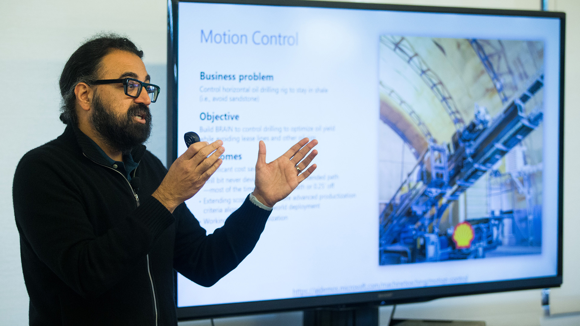
But as the desire to use AI for more scenarios has grown, Microsoft scientists and product developers have pioneered a complementary approach called machine teaching. This relies on people’s expertise to break a problem into easier tasks and give machine learning models important clues about how to find a solution faster. It’s like teaching a child to hit a home run by first putting the ball on the tee, then tossing an underhand pitch and eventually moving on to fastballs.
“This feels very natural and intuitive when we talk about this in human terms but when we switch to machine learning, everybody’s mindset, whether they realize it or not, is ‘let’s just throw fastballs at the system,’” said Mark Hammond, Microsoft general manager for Business AI. “Machine teaching is a set of tools that helps you stop doing that.”
Machine teaching seeks to gain knowledge from people rather than extracting knowledge from data alone. A person who understands the task at hand — whether how to decide which department in a company should receive an incoming email or how to automatically position wind turbines to generate more energy — would first decompose that problem into smaller parts. Then they would provide a limited number of examples, or the equivalent of lesson plans, to help the machine learning algorithms solve it.
In supervised learning scenarios, machine teaching is particularly useful when little or no labeled training data exists for the machine learning algorithms because an industry or company’s needs are so specific.
YouTube Video
In difficult and ambiguous reinforcement learning scenarios — where algorithms have trouble figuring out which of millions of possible actions it should take to master tasks in the physical world — machine teaching can dramatically shortcut the time it takes an intelligent agent to find the solution.
It’s also part of larger goal to enable a broader swath of people to use AI in more sophisticated ways. Machine teaching allows developers or subject matter experts with little AI expertise, such as lawyers, accountants, engineers, nurses or forklift operators, to impart important abstract concepts to an intelligent system, which then performs the machine learning mechanics in the background.
Microsoft researchers began exploring machine teaching principles nearly a decade ago, and those concepts are now working their way into products that help companies build everything from intelligent customer service bots to autonomous systems.
“Even the smartest AI will struggle by itself to learn how to do some of the deeply complex tasks that are common in the real world. So you need an approach like this, with people guiding AI systems to learn the things that we already know,” said Gurdeep Pall, Microsoft corporate vice president for Business AI. “Taking this turnkey AI and having non-experts use it to do much more complex tasks is really the sweet spot for machine teaching.”
Today, if we are trying to teach a machine learning algorithm to learn what a table is, we could easily find a dataset with pictures of tables, chairs and lamps that have been meticulously labeled. After exposing the algorithm to countless labeled examples, it learns to recognize a table’s characteristics.
But if you had to teach a person how to recognize a table, you’d probably start by explaining that it has four legs and a flat top. If you saw the person also putting chairs in that category, you’d further explain that a chair has a back and a table doesn’t. These abstractions and feedback loops are key to how people learn, and they can also augment traditional approaches to machine learning.
“If you can teach something to another person, you should be able to teach it to a machine using language that is very close to how humans learn,” said Patrice Simard, Microsoft distinguished engineer who pioneered the company’s machine teaching work for Microsoft Research. This month, his team moves to the Experiences and Devices group to continue this work and further integrate machine teaching with conversational AI offerings.
Microsoft researchers Patrice Simard, Alicia Edelman Pelton and Riham Mansour (left to right) are working to infuse machine teaching into Microsoft products. Photo by Dan DeLong for Microsoft.
Millions of potential AI users
Simard first started thinking about a new paradigm for building AI systems when he noticed that nearly all the papers at machine learning conferences focused on improving the performance of algorithms on carefully curated benchmarks. But in the real world, he realized, teaching is an equally or arguably more important component to learning, especially for simple tasks where limited data is available.
If you wanted to teach an AI system how to pick the best car but only had a few examples that were labeled “good” and “bad,” it might infer from that limited information that a defining characteristic of a good car is that the fourth number of its license plate is a “2.” But pointing the AI system to the same characteristics that you would tell your teenager to consider — gas mileage, safety ratings, crash test results, price — enables the algorithms to recognize good and bad cars correctly, despite the limited availability of labeled examples.
In supervised learning scenarios, machine teaching improves models by identifying these high-level meaningful features. As in programming, the art of machine teaching also involves the decomposition of tasks into simpler tasks. If the necessary features do not exist, they can be created using sub-models that use lower level features and are simple enough to be learned from a few examples. If the system consistently makes the same mistake, errors can be eliminated by adding features or examples.
One of the first Microsoft products to employ machine teaching concepts is Language Understanding, a tool in Azure Cognitive Services that identifies intent and key concepts from short text. It’s been used by companies ranging from UPS and Progressive Insurance to Telefonica to develop intelligent customer service bots.
“To know whether a customer has a question about billing or a service plan, you don’t have to give us every example of the question. You can provide four or five, along with the features and the keywords that are important in that domain, and Language Understanding takes care of the machinery in the background,” said Riham Mansour, principal software engineering manager responsible for Language Understanding.
Microsoft researchers are exploring how to apply machine teaching concepts to more complicated problems, like classifying longer documents, email and even images. They’re also working to make the teaching process more intuitive, such as suggesting to users which features might be important to solving the task.
Imagine a company wants to use AI to scan through all its documents and emails from the last year to find out how many quotes were sent out and how many of those resulted in a sale, said Alicia Edelman Pelton, principal program manager for the Microsoft Machine Teaching Group.
As a first step, the system has to know how to identify a quote from a contract or an invoice. Oftentimes, no labeled training data exists for that kind of task, particularly if each salesperson in the company handles it a little differently.
If the system was using traditional machine learning techniques, the company would need to outsource that process, sending thousands of sample documents and detailed instructions so an army of people can attempt to label them correctly — a process that can take months of back and forth to eliminate error and find all the relevant examples. They’ll also need a machine learning expert, who will be in high demand, to build the machine learning model. And if new salespeople start using different formats that the system wasn’t trained on, the model gets confused and stops working well.
By contrast, Pelton said, Microsoft’s machine teaching approach would use a person inside the company to identify the defining features and structures commonly found in a quote: something sent from a salesperson, an external customer’s name, words like “quotation” or “delivery date,” “product,” “quantity,” or “payment terms.”
It would translate that person’s expertise into language that a machine can understand and use a machine learning algorithm that’s been preselected to perform that task. That can help customers build customized AI solutions in a fraction of the time using the expertise that already exists within their organization, Pelton said.
Pelton noted that there are countless people in the world “who understand their businesses and can describe the important concepts — a lawyer who says, ‘oh, I know what a contract looks like and I know what a summons looks like and I can give you the clues to tell the difference.’”
Microsoft Corporate Vice President for Business AI Gurdeep Pall talks at a recent conference about autonomous systems solutions that employ machine teaching. Photo by Dan DeLong for Microsoft.
Making hard problems truly solvable
More than a decade ago, Hammond was working as a systems programmer in a Yale neuroscience lab and noticed how scientists used a step-by-step approach to train animals to perform tasks for their studies. He had a similar epiphany about borrowing those lessons to teach machines.
That ultimately led him to found Bonsai, which was acquired by Microsoft last year. It combines machine teaching with deep reinforcement learning and simulation to help companies develop “brains” that run autonomous systems in applications ranging from robotics and manufacturing to energy and building management. The platform uses a programming language called Inkling to help developers and even subject matter experts decompose problems and write AI programs.
Deep reinforcement learning, a branch of AI in which algorithms learn by trial and error based on a system of rewards, has successfully outperformed people in video games. But those models have struggled to master more complicated real-world industrial tasks, Hammond said.
Adding a machine teaching layer — or infusing an organization’s unique subject matter expertise directly into a deep reinforcement learning model — can dramatically reduce the time it takes to find solutions to these deeply complex real-world problems, Hammond said.
For instance, imagine a manufacturing company wants to train an AI agent to autonomously calibrate a critical piece of equipment that can be thrown out of whack as temperature or humidity fluctuates or after it’s been in use for some time. A person would use the Inkling language to create a “lesson plan” that outlines relevant information to perform the task and to monitor whether the system is performing well.
Armed with that information from its machine teaching component, the Bonsai system would select the best reinforcement learning model and create an AI “brain” to reduce expensive downtime by autonomously calibrating the equipment. It would test different actions in a simulated environment and be rewarded or penalized depending on how quickly and precisely it performs the calibration.
Telling that AI brain what’s important to focus on at the outset can short circuit a lot of fruitless and time-consuming exploration as it tries to learn in simulation what does and doesn’t work, Hammond said.
“The reason machine teaching proves critical is because if you just use reinforcement learning naively and don’t give it any information on how to solve the problem, it’s going to explore randomly and will maybe hopefully — but frequently not ever — hit on a solution that works,” Hammond said. “It makes problems truly solvable whereas without machine teaching they aren’t.”
The AWS DeepRacer League is the first of its kind global autonomous racing league, providing developers of all skill levels with the opportunity to get hands-on with machine learning and have fun doing it.
In another first for the AWS DeepRacer League, the race went truly global on April 17, 2019 as three live racing events got underway on the same day and in three different countries. We crowned three more AWS DeepRacer League champions. They are all heading to re:Invent 2019 on an expenses-paid trip to compete in the AWS DeepRacer Championship Cup final.
Following the sun to crown the champions
The races began in Seoul, South Korea, where developers were eager to get on the tracks in an attempt to beat the current world record set by the Singapore champion, Juv Chan.
Seoul was the second two day event on the summit circuit calendar. At the end of the qualifying rounds on the first day, the bar was set high. Racers then returned on the second day to try and capture the top spot. After the first day, “Steve’s” autonomous vehicle time was just under 10 seconds. He was about eight-tenths of a second from the current world record.
As the first day of racing in Seoul was nearly done, developers began competing in Dubai, UAE. Crowds gathered to watch developers put their skills to the test on the tracks. It was a close race in the top spots, but “Mats @ virgin mobile” emerged victorious with a winning time of 18.078 seconds. He trained his model at home using the Sagemaker RL notebook.
The Top 3 on the podium at Dubai
While the story unfolded in Dubai, the races in Amsterdam, Netherlands got underway. Another high-energy event, more developers gathered in Amsterdam to build, train, and deploy reinforcement learning models to their AWS DeepRacer fleet cars. The winner in Amsterdam, Pon Datalab, came to the summit with his colleagues to learn more about how AWS can improve data science for their business. He registered for a DeepRacer workshop with a few teammates because this was the first time any of them tried to build a machine learning model. When asked what the best part of his day was, Pon Datalab said “Going to the workshop, then working as a team to train our model, then seeing it in action, seeing it in first place was amazing, I cannot believe it!”
The Amsterdam champion “Pon Datalab”
Rounding out the triple with more record lap times
As we crowned the second of three champions, our competitors in Seoul were preparing for a final day of racing. The first day ended with the promise of an exciting day 2, as racers went home setting close to a record lap times and armed with new knowledge of how to improve their models from DeepRacer workshops, and experts at the track. The promise was kept, as 8 of our top 10 broke the 10 second barrier and our top 3 all smashed the previous record of 9.090 with sub 9 second laps!
Although all of our participants had some fantastic performances, there can be only one champion. He was Yejun Kim, who had started building his model 3 days prior to the summit using the SageMaker RL notebook. He attended a workshop and tweaked is racing model based on what he learnt there and improved his lap time each time he raced! His record time was 7.998 seconds!! He is now the AWS DeepRacer world record holder, and is excited to see what he can do when he gets to the finals at re:invent. Watch his winning lap time and listen to his excitement below.
#AWSDeepRacer world record has been set at 7.998 secs #Seoul, kudos to the winner and #AWSKorea team who provided all the support to developers. Watch out for the 3rd lap, that’s under 8secs. pic.twitter.com/B16nOXNfxl
Developers of all skill levels can race for prizes and glory, from anywhere in the world
The global developer community is achieving some amazing lap times. Can you? Whether you are new to machine learning or building on existing skills, you can race with enthusiasm and have fun doing it. Each summit champion is awarded an expenses-paid trip to the finals at re:Invent 2019 in Las Vegas, Nevada. There, the global champions compete for a chance to win the AWS DeepRacer Cup. It doesn’t matter whether you set a world record time or win by learning brand new skills.
Coming soon is the virtual league, where you can compete online through the AWS DeepRacer console. The virtual league gives you the same opportunity to compete and advance to the finals in Las Vegas, whatever continent or country you are in! With tracks varying in difficulty, and exciting themes that will be unveiled each month, the AWS DeepRacer League provides developers the opportunity to succeed.
About the Author
Alexandra Bush is a Senior Product Marketing Manager for AWS AI. She is passionate about how technology impacts the world around us and enjoys being able to help make it accessible to all. Out of the office she loves to run, travel and stay active in the outdoors with family and friends.

 Marisa Messina is on the AWS AI marketing team, where her job includes identifying the most innovative AWS-using customers and showcasing their inspiring stories. Prior to AWS, she worked on consumer-facing hardware and then university-facing cloud offerings at Microsoft. Outside of work, she enjoys exploring the Pacific Northwest hiking trails, cooking without recipes, and dancing in the rain.
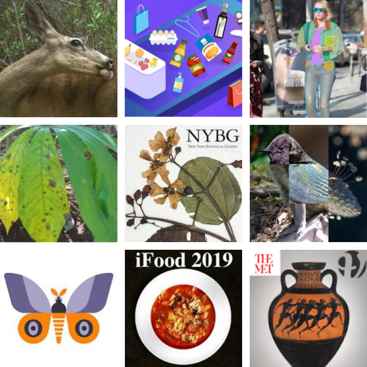


 Zach Kimberg is a Software Engineer with AWS Deep Learning working mainly on Apache MXNet for Java and Scala. Outside of work he enjoys reading, especially Fantasy.
 Sam Skalicky is a Software Engineer with AWS Deep Learning and enjoys building heterogeneous high performance computing systems. He is an avid coffee enthusiast and avoids hiking at all costs.
 Denis Davydenko is an Engineering Manager with AWS Deep Learning. He focuses on building Deep Learning tools that enable developers and scientists to build intelligent applications. In his spare time he enjoys spending time with his family, playing poker and video games.
 Sally Revell is a Senior Manager, Product Marketing for AWS AI. She loves to work on innovative products that have the potential to impact people’s lives in a positive way. In her spare time, she loves to do yoga, horseback riding and being outdoors in the beauty of the Pacific Northwest.


 Tristan Li is a Solutions Architect with Amazon Web Services. He works with enterprise customers in the US, helping them adopt cloud technology to build scalable and secure solutions on AWS.
 Wayne Davis is an Enterprise Solutions Architect for Amazon Web Services. Over the last 24 months he has been helping customers to come up to speed on cloud technologies as fast as possible.
 Robert Meagher is a software development engineer for AWS RoboMaker. He enjoys designing and tinkering with robotics systems, both in and out of the office.


 Sheeraz Ahmad is an applied scientist in the AWS AI Lab. He received his PhD from University of California, San Diego working at the intersection of machine learning and cognitive science, where he built computational models of how biological agents learn and make decisions. At Amazon, he works on improving the quality of crowdsourced data. In his spare time, Sheeraz loves to play board games, read science fiction, and lift weights.
 Lauren Moos is a software engineer with AWS AI. At Amazon, she has worked on a broad variety of machine learning problems, including machine learning algorithms for streaming data, consolidation of human annotations, and computer vision. Her primary interest is in machine learning’s relationship with cognitive science and modern philosophy. In her free time she reads, drinks coffee, and does yoga.


 Alexandra Bush is a Senior Product Marketing Manager for AWS AI. She is passionate about how technology impacts the world around us and enjoys being able to help make it accessible to all. Out of the office she loves to run, travel and stay active in the outdoors with family and friends.