Category: Global
Amazon SageMaker Ground Truth: Using A Pre-Trained Model for Faster Data Labeling
With Amazon SageMaker Ground Truth, you can build highly accurate training datasets for machine learning quickly. SageMaker Ground Truth offers easy access to public and private human labelers and provides them with built-in workflows and interfaces for common labeling tasks. Additionally, SageMaker Ground Truth can lower your labeling costs by up to 70% using automatic labeling, which works by training Ground Truth from data labeled by humans so that the service learns to label data independently. This previous blog post explains how automated data labeling works and how to evaluate its results.
What you may not know is that SageMaker Ground Truth trains models for you over the course of a labeling job, and that these models are available for use after a labeling job concludes! In this blog post, we will explain how you can use a model trained from a previous labeling job to “jump start” a subsequent labeling job. This is an advanced feature, only available through the SageMaker Ground Truth API.
| About this blog post | |
| Time to read | 30 minutes |
| Time to complete | 8 hours |
| Cost to complete | Under $600 |
| Learning level | Intermediate (200) |
| AWS services | Amazon SageMaker, Amazon SageMaker GroundTruth |
This post builds on the following prior post – you may find it useful to review it first:
As part of this blog, we will create three different labeling jobs, as described below.
- An initial labeling job with the “auto labeling” feature enabled. At the end of this labeling job, we will have a trained machine learning model capable of making high quality predictions on the sample dataset.
- A subsequent labeling job with a different set of images drawn from the same dataset as the first labeling job. In this labeling job, the machine learning model that was produced as an output of the first labeling job will be provided to accelerate the labeling process
- A repetition of the second labeling job, but without the pre-trained machine learning model. This labeling job is intended to serve as a control to demonstrate the benefit of using the pre-trained model.
We will use an Amazon SageMaker Jupyter notebook that uses the API to produce bounding box labels for our dataset.
To access the demo notebook, start an Amazon SageMaker notebook instance using an ml.m4.xlarge instance type. You can follow this step-by-step tutorial to set up an instance. On Step 3, make sure to mark “Any S3 bucket” when you create the IAM role! Open the Jupyter notebook, choose the SageMaker Examples tab, and launch object_detection_pretrained_model.ipynb.
Prepare Datasets
Let’s prepare our dataset to be used in creating our labeling jobs. We will create two sets of 1250 images from this dataset. We will use the first batch in our initial labeling job and the other batch for our two subsequent jobs, one with the pre-trained model and one without.
Next, run all the cells under ‘Prepare Dataset’ in the demo notebook. Running these cells will perform the following steps.
- Get the full collection of 2500 images from the dataset repository.
- Divide the dataset in two batches of 1250 images each.
Create An Initial Labeling Job With Active Learning
Now let’s run our first job. Run all of the cells under the “Iteration #1: Create Initial Labeling Job” heading of the notebook. You need to modify some of the cells, so read the notebook instructions carefully. Running these sections will perform the following steps.
- Prepare the first set of 1250 from the previous step for use in our first labeling job.
- Create labeling instructions for an object detection labeling job.
- Create an object detection labeling job request.
- Submit the labeling job request to SageMaker Ground Truth.
The job should take about four hours. When it’s done, run all of the cells in the “Analyze Initial Active Learning labeling job results” sections. These sections will produce a wealth of information that will help you understand the labeling job that you performed. In particular, we can see that the total cost was $217.18, of which 78% was attributable to the costs of manual labeling by the public work team. It’s worth pointing out that even at this stage there is modest cost savings due to our use of auto labeling – without it, the labeling cost would have been $235. In general, larger datasets (on the order of multiple thousands of objects) will be able to leverage greater use of auto labeling. In the rest of this blog, we will seek to improve the auto labeling performance even on this small 1,250-object dataset through the use of a pre-trained model.
In a previous blog post “Annotate data for less with Amazon SageMaker Ground Truth and automated data labeling” we described the batch-wise nature of a labeling job. In this blog post, we again refer to the batch-by-batch statistics of our labeling job. The plots below show that the model did not begin auto-labeling images until the 4th iteration. In the end, the ML model was able to annotate a little less than half of the entire dataset. We will look to increase the share of machine labeled data and consequently decrease the overall cost by using a pre-trained model in the next step.
Verify that the cell titled “Wait for Completion of Job” returns the job status “Completed” before proceeding to the next step.
Figure 1. Labeling costs and metrics for the initial labeling job.
Create A Second Labeling Job With A Pre-Trained Model
Now that the first labeling job is complete, we’ll prepare the second labeling job. We’ll reuse much of the original labeling job request, but we’ll need to specify the pre-trained machine learning model. We can query the original labeling job to get the Amazon ARN for the final machine learning model trained during the first job.
We’ll use this for the InitialActiveLearningModelArn parameter in the labeling job request.
In the demo notebook, run all the cells under the “Iteration #2: Labeling Job with Pre-Trained Model” heading. Running these sections will perform the following steps.
- Create an object detection labeling job request in which the model trained in the previous labeling job is provided.
- Submit the labeling job request to Ground Truth.
The job should take about four hours. When it’s done, run all of the cells in the “Analyze Active Learning labeling job with pre-trained model results” sections. This will produce a wealth of information similar to what we saw after the previous labeling job. You should already see some key differences in the number of machine-labeled dataset objects! In particular, the machine learning model is able to start labeling data in the third iteration, and when it does, it annotates almost the entire remainder of the dataset! Note that the cost associated with manual labeling is much lower than before. Although the cost associated with auto labeling has increased, this increase is smaller in magnitude than the decrease in the human labeling cost. Consequently, the overall cost of this labeling job – $146.80 – is 33% lower than that of the first labeling job.
Verify that the cell titled “Wait for Completion of Job” returns the job status “Completed” before proceeding to the next step.
Figure 2. Labeling costs and metrics for the second labeling job with the use of a pre-trained model.
Repeat the Second Labeling Job Without the Pre-Trained Model
In the previous labeling job, we saw a substantial improvement in run time and the number of machine labeled dataset objects relative to the first dataset. However, one may naturally ask how much of the difference is due to the difference in the underlying data. Although both datasets have the same labels and are sampled from the same, larger dataset, a controlled study will provide a fairer assessment. To that end, we’ll now repeat the second labeling job with all the same settings, but remove the pre-trained model. In the demo notebook, run all the cells in the “Labeling Job without Pre-trained model”. Running these sections will perform the following steps.
- Duplicate the labeling job request from the second labeling job with the removal of the pre-trained model.
- Submit the labeling job request to Ground Truth
The job should take about four hours. When it’s done, run all of the cells under the “Iteration #3: Second Data Subset Without Pre-Trained Model” heading. Again, this will produce plots that look similar to those generated in the previous steps. However, these figures should look more similar to the results of the first labeling job than the second. Notice that the overall cost is $189.64, and that the job took five iterations to complete. Notice that this is 29% larger than when we used the pre-trained model to help label this data!
Figure 3. Labeling costs and metrics for the third labeling job, which uses the same dataset as the second labeling job without the benefit of the pre-trained model.
Compare Results
Now that we’ve run all there labeling jobs, we can compare the results more fully. First, consider the left-hand plot shown below. The total elapsed running time for the labeling job that uses the pre-trained model is less than half the time required for the jobs that don’t make use of the pre-trained model. We can also see in the right-hand plot below that this reduction in time goes hand-in-hand with a larger fraction of auto-labeled data. The reason that the labeling job that uses the pre-trained model is so much faster is because the machine learning model does more of the work, which is much more efficient than manual labeling.
It should be noted that some amount of variability is expected in these results. Due to the small random effects introduced by the pool of workers available when these labeling jobs were performed, the small fluctutations that may be seen in training the machine learning model, etc., a repeated trial of these three labeling jobs may result in slightly different numbers. However, the substantial gain in cost and time savings seen in experiment #2 is predominately due to the use of the pre-trained model.

Figure 4. Comparison of labeling time and auto-labeling efficiency across the three labeling jobs.
Finally, the plot below shows that the reduction in labeling time and the increase in the fraction of data annotated by the machine learning model lead to a measurable reduction in the total labeling cost. In this example we see that when labeling the second dataset, using a pre-trained model leads to a 23% reduction in cost relative to the control scenario where the pre-trained model was not used – $146.80 vs $189.64.
Figure 5. Total labeling cost across the three labeling jobs.
Conclusion
Let’s review what we covered in this exercise.
- We gathered a dataset consisting of 2500 images of birds from the Open Images dataset.
- We split this dataset into two halves.
- We created an object detection labeling job for the first subset of 1250 images and saw that approximately 48% of the dataset was machine-labeled.
- We created a second labeling job for the second subset, and we specified the machine learning model that was trained during the first labeling job. This time we found that approximately 80% of the dataset was machine-labeled.
- As a final benchmark, we re-ran the second labeling job without specifying the pre-trained model. Now we found that approximately 60% of the dataset was machine-labeled.
- In the end, we saw a 50% reduction in time required to acquire labels, and a 23% reduction in total labeling cost when we use a pre-trained model. This is highly context dependent, and results will vary from application to application. However, the workflow illustrated in this example demonstrates the value of using a pre-trained model for successive labeling jobs.
If we were to acquire a new unlabeled dataset in this domain (e.g., object detection for birds), we could setup another labeling job, and specify the model trained in our second labeling job. The use of pre-trained machine learning models thus allows you to run labeling jobs in succession, with each job improving from the predictive ability gained through the previous job. Remember that the pre-trained model capability requires you to use the “job chaining” feature (described in https://aws.amazon.com/blogs/aws/amazon-sagemaker-ground-truth-keeps-simplifying-labeling-workflows/) or to use the Amazon SageMaker Ground Truth API, as we demonstrated in the accompanying example notebook.
About the Authors
 Prateek Jindal is a software development engineer for AWS AI. He is working on solving complex data labeling problems in the machine learning world and has a keen interest in building scalable distributed solutions for his customers. In his free time, he loves to cook, try out new restaurants, and hit the gym.
 Jonathan Buck is a software engineer at Amazon. His focus is on building impactful software services and products to democratize machine learning.
Striking a Chord: Anthem Helps Patients Navigate Healthcare with Ease
AI is bringing convenience to your healthcare experience.
Health insurance company Anthem helps patients personalize and better understand their healthcare information through AI.
Operating in 14 states with more than 40 million members on its health plans, Anthem is developing into “AI and digital-first company” to better assist their customers.
“We have to acknowledge that our legacy has been that we’re an insurance company, and we’re quite good at it,” said Rajeev Ronanki, senior vice president and chief digital officer at Anthem, in a conversation with AI Podcast host Noah Kravitz. “But more and more the world is evolving to where insurance is really about data. And to make data meaningful and useful, we need AI, hence the transformation.”
Ronanki believes that “digital data and AI are the bridge” to solving the issues in the healthcare industry, and that, in the future, the medical field will employ a variety of AI-assisted tools to augment patient care.
“Almost no one gives the US healthcare system high marks,” Ronanki said. “Hard to use, hard to understand, it’s too expensive — the system is just broken.”
“If we can think of healthcare as a supply and demand problem, and systematically digitize all the supply points so your doctors’ offices, hospitals, retail, clinics… and make all of that supply available in a consistent and systematic manner to the demand of the patients, then we can thrive.”
Acknowledging the concerns over data privacy, Ronanki stressed Anthem’s mission for patients to have greater transparency into and full control over their own entire health history.
“That’s the paradigm shift that we want to make,” said Ronanki. “Which is to liberate data from all the places that it exists today, and make it available to consumers and let them make the choice and to who to make that data available to.”
Later this fall, Anthem plans to launch their AI-powered product that gives users the opportunity to diagnose themselves, schedule video consultations, and book doctors’ appointments all with a few clicks of a button.
Help Make the AI Podcast Better
Have a few minutes to spare? It’d help us if you fill out this short listener survey.
Your answers will help us learn more about our audience, which will help us deliver podcasts that meet your needs, what we can do better, and what we’re doing right.
How to Tune into the AI Podcast
Our AI Podcast is available through iTunes, Castbox, DoggCatcher, Google Play Music, Overcast, PlayerFM, Podbay, PodBean, Pocket Casts, PodCruncher, PodKicker, Stitcher, Soundcloud and TuneIn.
If your favorite isn’t listed here, email us at aipodcast [at] nvidia [dot] com.
The post Striking a Chord: Anthem Helps Patients Navigate Healthcare with Ease appeared first on The Official NVIDIA Blog.
Startup Takes On Cancer Treatment Procedure With Quadro RTX-Powered AI
As more physicians turn to the latest advancements in technology to improve medical practices, one company is bringing the power of AI to the fight against cancer.
Most people know that chemotherapy and surgery are used to treat cancer, but thermal ablation is often under the radar. It’s a minimally invasive process that applies intense heat to tissue to remove early-stage tumors.
Thermal ablation is a safe, effective procedure that’s quickly becoming one of the best alternative treatments for cancer, especially for patients who are unable to undergo surgery.
To date, doctors performing thermal ablation typically haven’t had the tools to visualize or control the damage created during the procedure. This means tumor removal could be incomplete or healthy tissue could be harmed. Plus, physicians needed to wait up to 24 hours to see how effective the procedure was on the targeted tissue.
To address this challenge, Israel-based company TechsoMed has developed BioTrace, the world’s first real-time monitoring and control system for thermal ablation.
With the help of NVIDIA Quadro RTX 8000 GPUs, BioTrace uses AI algorithms applied to image data from ultrasound devices to perform monitoring and analysis during thermal ablation procedures.
The technology tracks the real-time biological response of the tissue so physicians can have better visibility and understand the results of the cancer treatment as it’s performed.
RTX Brings Real-Time Results
For BioTrace to process data instantly and provide real-time feedback, TechsoMed runs advanced AI algorithms using dual NVIDIA Quadro RTX 8000 graphics packed inside a Lenovo ThinkStation P920 workstation.
Quadro RTX 8000 is the world’s most powerful GPU based on NVIDIA’s latest Turing architecture and features Tensor Cores specifically designed to accelerate AI algorithms.
TechsoMed uses two RTX 8000 GPUs paired with NVIDIA NVLink high-speed interconnect technology to scale up performance and memory capacity to 96GB, which is critical when working with massive image data in real time.
“BioTrace is taking the guesswork out of ablation procedures through AI algorithms and image processing technologies, and the NVIDIA RTX GPUs help make it possible,” said Yossi Abu, founder and CEO of TechsoMed. “By defining the exact algorithm practitioners need to visualize the results, RTX enables our work to bring thermal ablation procedures to a new level.”
The real-time feedback from BioTrace brings benefits such as faster recovery, fewer potential complications and less damage to surrounding healthy tissue. With RTX powering their simulations, doctors can take advantage of higher resolution images and real-time feedback to improve accuracy and minimize damage.
Find more information about TechsoMed’s BioTrace or learn more about NVIDIA RTX.
The post Startup Takes On Cancer Treatment Procedure With Quadro RTX-Powered AI appeared first on The Official NVIDIA Blog.
Innovations in Graph Representation Learning
Relational data representing relationships between entities is ubiquitous on the Web (e.g., online social networks) and in the physical world (e.g., in protein interaction networks). Such data can be represented as a graph with nodes (e.g., users, proteins), and edges connecting them (e.g., friendship relations, protein interactions). Given the widespread prevalence of graphs, graph analysis plays a fundamental role in machine learning, with applications in clustering, link prediction, privacy, and others. To apply machine learning methods to graphs (e.g., predicting new friendships, or discovering unknown protein interactions) one needs to learn a representation of the graph that is amenable to be used in ML algorithms.
However, graphs are inherently combinatorial structures made of discrete parts like nodes and edges, while many common ML methods, like neural networks, favor continuous structures, in particular vector representations. Vector representations are particularly important in neural networks, as they can be directly used as input layers. To get around the difficulties in using discrete graph representations in ML, graph embedding methods learn a continuous vector space for the graph, assigning each node (and/or edge) in the graph to a specific position in a vector space. A popular approach in this area is that of random-walk-based representation learning, as introduced in DeepWalk.
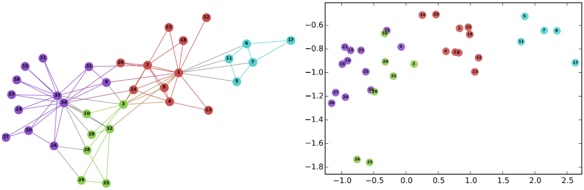 |
| Left: The well-known Karate graph representing a social network. Right: A continuous space embedding of the nodes in the graph using DeepWalk. |
Here we present the results of two recent papers on graph embedding: “Is a Single Embedding Enough? Learning Node Representations that Capture Multiple Social Contexts” presented at WWW’19 and “Watch Your Step: Learning Node Embeddings via Graph Attention” at NeurIPS’18. The first paper introduces a novel technique to learn multiple embeddings per node, enabling a better characterization of networks with overlapping communities. The second addresses the fundamental problem of hyperparameter tuning in graph embeddings, allowing one to easily deploy graph embeddings methods with less effort. We are also happy to announce that we have released the code for both papers in the Google Research github repository for graph embeddings.
Learning Node Representations that Capture Multiple Social Contexts
In virtually all cases, the crucial assumption of standard graph embedding methods is that a single embedding has to be learned for each node. Thus, the embedding method can be said to seek to identify the single role or position that characterizes each node in the geometry of the graph. Recent work observed, however, that nodes in real networks belong to multiple overlapping communities and play multiple roles—think about your social network where you participate in both your family and in your work community. This observation motivates the following research question: is it possible to develop methods where nodes are embedded in multiple vectors, representing their participation in overlapping communities?
In our WWW’19 paper, we developed Splitter, an unsupervised embedding method that allows the nodes in a graph to have multiple embeddings to better encode their participation in multiple communities. Our method is based on recent innovations in overlapping clustering based on ego-network analysis, using the persona graph concept, in particular. This method takes a graph G, and creates a new graph P (called the persona graph), where each node in G is represented by a series of replicas called the persona nodes. Each persona of a node represents an instantiation of the node in a local community to which it belongs. For each node U in the graph, we analyze the ego-network of the node (i.e., the graph connecting the node to its neighbors, in this example A, B, C, D) to discover local communities to which the node belongs. For instance, in the figure below, node U belongs to two communities: Cluster 1 (with the friends A and B, say U’s family members) and Cluster 2 (with C and D, say U’s colleagues).
 |
| Ego-net of node U |
Then, we use this information to “split” node U into its two personas U1 (the family persona) and U2 (the work persona). This disentangles the two communities, so that they no longer overlap.
 |
| The ego-splitting method separating the U nodes in 2 personas. |
This technique has been used to improve the state-of-the-art results in graph embedding methods, showing up to 90% reduction in link prediction (i.e., predicting which link will form in the future) error on a variety of graphs. The key reason for this improvement is the ability of the method to disambiguate highly overlapping communities found in social networks and other real-world graphs. We further validate this result with an in-depth analysis of co-authorship graphs where authors belong to overlapping research communities (e.g., machine learning and data mining).
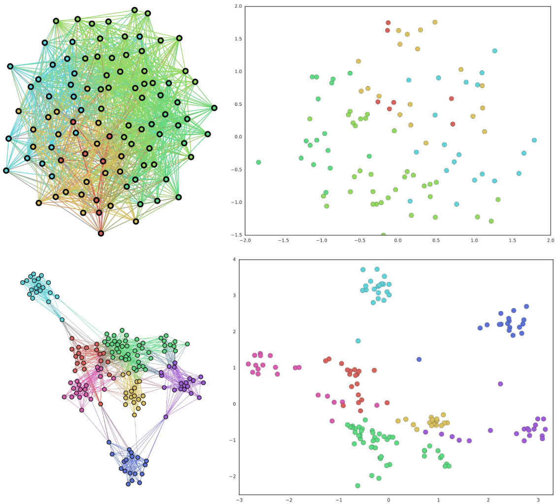 |
| Top Left: A typical graphs with highly overlapping communities. Top Right: A traditional embedding of the graph on the left using node2vec. Bottom Left: A persona graph of the graph above. Bottom Right: The Splitter embedding of the persona graph. Notice how the persona graph clearly disentangles the overlapping communities of the original graph and Splitter outputs well-separated embeddings. |
Automatic hyper-parameter tuning via graph attention.
Graph embedding methods have shown outstanding performance on various ML-based applications, such as link prediction and node classification, but they have a number of hyper-parameters that must be manually set. For example, are nearby nodes more important to capture when learning embeddings than nodes that are further away? Even though experts may be able to fine tune these hyper-parameters, one must do so independently for each graph. To obviate such manual work, in our second paper, we proposed a method to learn the optimal hyper-parameters automatically.
Specifically, many graph embedding methods, like DeepWalk, employ random walks to explore the context around a given node (i.e. the direct neighbors, the neighbors of the neighbors, etc). Such random walks can have many hyper-parameters that allow tuning of the local exploration of the graph, thus regulating the attention given by the embeddings to nearby nodes. Different graphs may present different optimal attention patterns and hence different optimal hyperparameters (see the picture below, where we show two different attention distributions). Watch Your Step formulates a model for the performance of the embedding methods based on the above mentioned hyper-parameters. Then we optimize the hyper-parameters to maximize the performance predicted by the model, using standard backpropagation. We found that the values learned by backpropagation agree with the optimal hyper-parameters obtained by grid search.
 |
| Our new method for automatic hyper-parameter tuning, Watch Your Step, uses an attention model to learn different graph context distributions. Shown above are two example local neighborhoods about a center node (in yellow) and the context distributions (red gradient) that was learned by the model. The left-side graph shows a more diffused attention model, while the distribution on the right shows one concentrated on direct neighbors. |
This work falls under the growing family of AutoML, where we want to alleviate the burden of optimizing the hyperparameters—a common problem in practical machine learning. Many AutoML methods use neural architecture search. This paper instead shows a variant, where we use the mathematical connection between the hyperparameters in the embeddings and graph-theoretic matrix formulations. The “Auto” portion corresponds to learning the graph hyperparameters by backpropagation.
We believe that our contributions will further advance the state of the research in graph embedding in various directions. Our method for learning multiple node embeddings draws a connection between the rich and well-studied field of overlapping community detection, and the more recent one of graph embedding which we believe may result in fruitful future research. An open problem in this area is the use of multiple-embedding methods for classification. Furthermore, our contribution on learning hyperparameters will foster graph embedding adoption by reducing the need for expensive manual tuning. We hope the release of these papers and code will help the research community pursue these directions.
Acknowledgements
We thank Sami Abu-el-Haija who contributed to this work and is now a Ph.D. student at USC.

How Siemens Healthineers Is Streamlining Cancer Therapy with AI
Cancer incidence rates are on the rise — expected to increase by 63 percent over the next two decades. To meet the growing demand for care, medical technology leaders are turning to AI tools that can help radiation oncologists provide high-quality, individualized treatment faster.
One of the world’s leading healthcare companies, Siemens Healthineers, is using an NVIDIA GPU-based supercomputing infrastructure to develop AI software for generating organ segmentations that enable precision radiation therapy.
Siemens Healthineers’ Sherlock AI supercomputer is powered by NVIDIA HGX 1 and HGX 2 servers loaded with NVIDIA V100 Tensor Core GPUs. The system provides 20 petaflops of performance and is used to run over 500 AI experiments daily.
Both Siemens Healthineers and NVIDIA this week are sharing their latest work in AI for medical imaging at the Society for Imaging Informatics in Medicine annual conference, held outside Denver, Colorado. The event brings together the medical informatics community to share, debate, and address the challenges and opportunities facing medical imaging.
Augmenting Radiation Therapy Workflows
Radiation therapy for cancer patients is a complex workflow that includes modeling the patient, contouring the target and organs at risk, simulating the treatment, planning and delivering the treatment.
One of the most time-consuming tasks in this process is protecting the healthy organs at risk that surround a patient’s tumor and need to be spared from excessive radiation dose. Traditionally, radiation oncologists contour the tumor target volume and organs at risk, deciding how much radiation should be used to treat tumors without damaging neighboring normal tissue.
To help oncologists develop radiation treatment plans faster, Siemens Healthineers uses syngo.via RT Image Suite, a software tool that automatically outlines organs using AI-assisted AutoContouring. Trained on over 4.5 million images using the Sherlock supercomputer, the AI model saves radiation-oncologist time and eases organs-at-risk contouring tasks. In their current research, Siemens Healthineers automatically outlines 28 organs using AI technology.
“AI-assisted AutoContouring helps save time and improve standardization in organ at risk contouring,” said Dr. Fernando Vega, Head of Software and Concept Definition for Radiation Oncology at Siemens Healthineers. “This allows radiation-oncologists to better focus on other crucial aspects of patient care.”
Tapping into Software To Write Software
Behind this explosion of AI in medical imaging is a new dynamic within the software development paradigm: the advent of software that writes other software.
Traditionally, engineers have written applications from start to finish, a time-consuming process that requires niche computing expertise. Now, with access to powerful compute resources, AI algorithms can leverage training data to learn processes like medical image analysis without every element being explicitly coded by a developer.
Siemens Healthineers, which has been involved in machine learning since the 1990s, is harnessing this AI capability with the Sherlock system. The supercomputer learns from the company’s massive data lake of over 750 million curated images as well as radiology reports and clinical and genomic data. So far, it has led to the development of more than 40 AI-powered applications approved for clinical use.
“We believe that AI is starting a new era in software development, where advanced neural network architectures, large collections of curated data, and massive computational power come together to deliver tremendous performance and high clinical value,” said Dr. Dorin Comaniciu, Senior Vice President of artificial intelligence and digital innovation at Siemens Healthineers.
Simple and Scalable Infrastructure
Siemens Healthineers’ 20 petaflop Sherlock supercomputer addresses a key computing need in the healthcare industry for an optimized and scalable infrastructure that can be used to develop deep learning tools for imaging and other clinical applications.
The NVIDIA DGX POD reference architecture provides a tested infrastructure for setting up a scalable AI computing system. Through the DGX-Ready Data Center program, NVIDIA and its colocation service providers offer simplified, rapid deployment for customers building and deploying world-class AI data centers for the healthcare industry.
For more on how NVIDIA’s AI platform is enabling advances in medicine and research, see the NVIDIA Healthcare page.
The post How Siemens Healthineers Is Streamlining Cancer Therapy with AI appeared first on The Official NVIDIA Blog.
Another triple for the DeepRacer League brings more world records and the first female winner!
The AWS DeepRacer League is the world’s first global autonomous racing league, open to anyone. Developers of all skill levels can compete in person at 22 AWS events globally, or online via the AWS DeepRacer console, for a chance to win an expense paid trip to re:Invent 2019, where they will race to win the Championship Cup 2019.
Last week the AWS DeepRacer League visited three cities around the world – Washington D.C, USA, Taipei, Taiwan, and Tokyo, Japan. Each race spanned multiple days, providing developers with numerous opportunities to record a winning lap time.
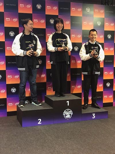
The first female winner and another world record
The Tokyo race was the biggest one yet. Over 20,000 AWS customers came to the AWS Summit at the Makuhari Messe, located just outside of the city, for three days of learning, hands-on labs, and networking. There were two DeepRacer tracks for developers to race on throughout the summit, virtual racing pods, and multiple workshops to learn how to build a DeepRacer model.

Virtual racing pods, for customers to build models and learn more about the AWS DeepRacer league.
Hundreds of developers tested out their model on the tracks, but none could take the top spot from our first female winner, sola@DNP, who took home the cup with a world record winning time of 7.44 seconds – that means DeepRacer is travelling at the equivalent of roughly 100mph if scaled up to a real size car! Here is sola@DNP celebrating on the podium with her teammates. Check out the lightning fast winning lap!
We have a new world record where the current champion set 7.5 and 7.44sec laps in her trials. #AWSDeepRacer #Tokyo pic.twitter.com/j8e96fKB0u
— sunil mallya (@sunilmallya) June 14, 2019
She came to the AWS Summit as part of a team created at her company DNP (Dai Nippon Printing, a Japanese printing company operating in areas such as Information Communications, Lifestyles and Industrial Supplies and, Electronics). 28 of them placed on the leaderboard, with the top 3 all being from the team – 2 of them beating the previous world record (7.62 seconds) set just the week before at Amazon re:MARS.
To prepare for such a strong showing, DNP created DeepRacer study groups where employees share their knowledge and newly acquired machine learning skills. They see DeepRacer as a fun and engaging way to grow their engineers’ skills in AI.
“We currently have around 2000 IT personnel in the group and fewer than 200 employees experienced in working with AI. We want to double the number within 5 years.” – Mr. Shinichiro Fukuda, Deputy Director, C & I Center, DNP Information Innovation Division

Race Stats
The race in Japan was the most competitive yet. The top 33 competitors achieved lap times of under 10 seconds, the top 17 were under 9 seconds and the top 4 were under 8 seconds – breaking the world record twice! Check out the fast times and final results from the race on the Tokyo Leaderboard.
Washington DC
The AWS Public Sector Summit in Washington DC on June 10 also had an exciting race and there was a familiar face back on the tracks – our second place winner at Amazon re:MARS, John Amos. John narrowly missed out on the win and the opportunity to compete at re:Invent, in Las Vegas, when Anthony Navarro beat his world record time in the last few minutes of racing. In Washington, he took the lead early on and held his position steadfast in his pursuit of the win and will now be winging his way to re:Invent with the other Summit and Virtual circuit winners. He is really enjoying his AWS DeepRacer experience and has a new hobby to boot!
“I think everyone should have a hobby and this is a healthy one. There’s lots of stuff you can get addicted to, but with this you’re out there running models using technology. I’m used to playing video games online, but this helps it become real. What you do in the reward function impacts what’s happening with the car, so taking it from the simulator out onto the track is just exhilarating, and who doesn’t love a good challenge?”

Taipei
In Taipei, developers were also burning rubber and posting fast times on the leaderboard, and the winner took the top spot by a narrow margin (just 0.04 of a second), and in an exciting last few minutes of the race! He was Roger@NCTU_CGI, with a winning time of 8.734 seconds. Congratulations to all of the winners this week, it’s going to be an exciting final round at re:Invent 2019.

The AWS DeepRacer League Summit Circuit is in the homestretch
The AWS DeepRacer League Summit circuit only has five more races, (Hong Kong, Cape Town, New York, Mexico City, and Toronto) before the finale in Las Vegas, and it is shaping up to be an exciting event. Join the league at one of the 5 remaining races on the summit circuit, or race online in the virtual circuit today for your chance to win your trip to compete!
About the Author
 Alexandra Bush is a Senior Product Marketing Manager for AWS AI. She is passionate about how technology impacts the world around us and enjoys being able to help make it accessible to all. Out of the office she loves to run, travel and stay active in the outdoors with family and friends.
Quantib’s Quest: Startup Assists Radiologists in Detecting Dementia
Dementia diagnosis starts with uncertainty — patients or their family members make an appointment after noticing symptoms that suggest something’s wrong.
It may take months or years to reach a final diagnosis, as doctors must observe how a patient’s condition progresses over time.
Radiologists don’t typically have serial quantitative brain data — calculated measurements of a patient’s brain structures taken at different times — on hand during this process. They rely instead on visual assessments of the scans, rating a patient’s brain atrophy levels on a four or five-point scale.
Experts rely on these qualitative scores because even when serial scans are available, it would radiologists inordinately long to quantify the data, as they have to calculate brain structure volumes by hand.
“It’d just be too expensive to let radiologists do that,” said Jorrit Glastra, chief technology officer of Quantib, a Netherlands-based startup using deep learning to tackle this problem.
AI can accelerate the analysis of brain MRI data, taking just a few minutes to generate a report of structure volumes for radiologists and neurologists, who work together to study a patient’s scans and cognitive test results. Looking at the hard numbers can help experts more easily measure the change in a patient’s brain over time, shortening the time to diagnosis.
“The longer disease diagnosis is delayed, the more care a patient will need and the higher the costs,” Glastra said. “It’s very valuable to diagnose cases early.”
A member of the NVIDIA Inception program, Quantib trains its deep learning algorithms on NVIDIA V100 and K80 GPUs. Its deep learning software, Quantib ND, is FDA cleared in the United States and CE marked in Europe.
The company’s technology is installed in around 20 countries across Europe, North America and Asia.
AI’ll Do the Math
Dementia affects 50 million people worldwide — a figure expected to grow in coming years as life expectancy rises. Artificial intelligence tools like Quantib ND can help radiologists monitor disease progress in patients and diagnose new cases earlier.
Quantib ND quantifies brain atrophy by segmenting brain structures and white matter hyperintensities, which signify the level of disease-induced damage in the brain.
Radiologists can also use the tool to compare a patient’s brain tissue volumes to a reference library of MRI scans. This database makes it easier to determine whether a patient’s brain is showing normal aging or not.
Based on a dataset of 5,000 brain scans, Quantib ND’s AI can differentiate between brain atrophy patterns indicative of Alzheimer’s disease and ones associated with other kinds of dementia. The tool can also be used to compare an individual patient’s scans over time to determine how a disease is progressing.
Beyond the Brain
Quantib is also building deep learning solutions for oncologists detecting prostate cancer and breast cancer. Its AI algorithm for prostate cancer, currently in development, can segment, classify and predict the state of suspicious lesions from MRI scans. Doctors can then use these insights to determine which lesions to target with a biopsy.
The company’s breast cancer screening AI analyzes MRI scans for women with high breast density — an independent risk factor for developing breast cancer. Radiologists and oncologists use these scans to determine if a patient will require a biopsy.
Glastra said for both breast and prostate cancer screening, the AI must analyze a set of multiple images from different time points. The complexity of the deep learning task demands powerful computation tools for inference.
“For breast cancer screening, the data volume going into that set of scans is unbelievable. It’s several orders of magnitude higher than the brain,” he said. “Running inference on the types of models that can handle those inputs can only be done with GPU support.”
Quantib benchmarked the performance of its prostate cancer AI using the 70-watt NVIDIA T4 GPUs for inference — and found the algorithms run 24x faster compared to using a CPU cluster with the same power usage.
“For on-premises inference,” Glastra said, “the low-power footprint of the T4 makes it a very attractive option.”
The post Quantib’s Quest: Startup Assists Radiologists in Detecting Dementia appeared first on The Official NVIDIA Blog.
Train and deploy Keras models with TensorFlow and Apache MXNet on Amazon SageMaker
Keras is a popular and well-documented open source library for deep learning, while Amazon SageMaker provides you with easy tools to train and optimize machine learning models. Until now, you had to build a custom container to use both, but Keras is now part of the built-in TensorFlow environments for TensorFlow and Apache MXNet. Not only does this simplify the development process, it also allows you to use standard Amazon SageMaker features like script mode or automatic model tuning.
Keras’s excellent documentation, numerous examples, and active community make it a great choice for beginners and experienced practitioners alike. The library provides a high-level API that makes it easy to build all kind of deep learning architectures, with the option to use different backends for training and prediction: TensorFlow, Apache MXNet, and Theano.
In this post, I show you how to train and deploy Keras 2.x models on Amazon SageMaker, using the built-in TensorFlow environments for TensorFlow and Apache MXNet. In the process, you also learn the following:
- To run the same Keras code on Amazon SageMaker that you run on your local machine, use script mode.
- To optimize hyperparameters, launch automatic model tuning.
- Deploy your models with Amazon Elastic Inference.
The Keras example
This example demonstrates training a simple convolutional neural network on the Fashion MNIST dataset. This dataset replaces the well-known MNIST dataset. It has the same number of classes (10), samples (60,000 for training, 10,000 for validation), and image properties (28×28 pixels, black and white). But it’s also much harder to learn, which makes for a more interesting challenge.
First, set up TensorFlow as your Keras backend (and switch to Apache MXNet later on). For more information, see the mnist_keras_tf_local.py script.
The process is straightforward:
- Grab optional parameters from the command line, or use default values if they’re missing.
- Download the dataset and save it to the /data directory.
- Normalize the pixel values, and one hot encode labels.
- Build the convolutional neural network.
- Train the model.
- Save the model to TensorFlow Serving format for deployment.
Positioning your image channels can be tricky. Black and white images have a single channel (black), while color images have three channels (red, green, and blue). The library expects data to have a well-defined shape when training a model, describing the batch size, the height and width of images, and the number of channels. TensorFlow specifically requires the input shape formatted as (batch size, width, height, channels), with channels last. Meanwhile, MXNet expects (batch size, channels, width, height), with channels first. To avoid training issues created by using the wrong shape, I add a few lines of code to identify the active setting and reshape the dataset to compensate.
Now check that this code works by running it on a local machine, without using Amazon SageMaker.
Training and deploying the Keras model
You must make a few minimal changes, but script mode does most of the work for you. Before invoking your code inside the TensorFlow environment, Amazon SageMaker sets four environment variables
- SM_NUM_GPUS—The number of GPUs present on the instance.
- SM_MODEL_DIR— The output location for the model.
- SM_CHANNEL_TRAINING— The location of the training dataset.
- SM_CHANNEL_VALIDATION—The location of the validation dataset.
You can use these values in your training code with just a simple modification:
What about hyperparameters? No work needed there. Amazon SageMaker passes them as command line arguments to your code.
For more information, see the updated script, mnist_keras_tf.py.
Training on Amazon SageMaker
After deploying your Keras model, you can begin training on Amazon SageMaker. For more information, see the Fashion MNIST-SageMaker.ipynb notebook.
The process is straightforward:
- Download the dataset.
- Define the training and validation channels.
- Configure the TensorFlow estimator, enabling script mode and passing some hyperparameters.
- Train, deploy, and predict.
In the training log, you can see how Amazon SageMaker sets the environment variables and how it invokes the script with the three hyper parameters defined in the estimator:
Because you saved your model in TensorFlow Serving format, Amazon SageMaker can deploy it just like any other TensorFlow model by calling the deploy() API on the estimator. Finally, you can grab some random images from the dataset and predict them with the model you just deployed.
Script mode makes it easy to train and deploy existing TensorFlow code on Amazon SageMaker. Just grab those environment variables, add command line arguments for your hyperparameters, save the model in the right place, and voilà!
Switching to the Apache MXNet backend
As mentioned earlier, Keras also supports MXNet as a backend. Many customers find that it trains faster than TensorFlow, so you may want to give it a shot.
Everything discussed above still applies (script mode, etc.). You only make two changes:
- Use channels_first.
- Save the model in MXNet format, creating an extra file (model-shapes.json) required to load the model for prediction.
For more information, see the mnist_keras_mxnet.py training code for MXNet.
You can find the Amazon SageMaker steps in the notebook. Apache MXNet uses virtually the same process I just reviewed, aside from using the MXNet estimator.
Automatic model tuning on Keras
Automatic model tuning is a technique that helps you find the optimal hyperparameters for your training job, that is, the hyperparameters that maximize validation accuracy.
You have access to this feature by default because you’re using the built-in estimators for TensorFlow and MXNet. For the sake of brevity, I only show you how to use it with Keras-TensorFlow, but the process is identical for Keras-MXNet.
First, define the hyperparameters you’d like to tune, and their ranges. How about all of them? Thanks to script mode, your parameters are passed as command line arguments, allowing you to tune anything.
When configuring automatic model tuning, define which metric to optimize on. Amazon SageMaker supports predefined metrics that it can read automatically from the training log for built-in algorithms (XGBoost, etc.) and frameworks (TensorFlow, MXNet, etc.). That’s not the case for Keras. Instead, you must tell Amazon SageMaker how to grab your metric from the log with a simple regular expression:
Then, you define your tuning job, run it, and deploy the best model. No difference here.
Advanced users may insist on using early stopping to avoid overfitting, and they would be right. You can implement this in Keras using a built-in callback (keras.callbacks.EarlyStopping). However, this also creates difficulty in automatic model tuning.
You need Amazon SageMaker to grab the metric for the best epoch, not the last epoch. To overcome this, define a custom callback to log the best validation accuracy. Modify the regular expression accordingly so that Amazon SageMaker can find it in the training log.
For more information, see the 02-fashion-mnist notebook.
Conclusion
I covered a lot of ground in this post. You now know how to:
- Train and deploy Keras models on Amazon SageMaker, using both the TensorFlow and the Apache MXNet built-in environments.
- Use script mode to use your existing Keras code with minimal change.
- Perform automatic model tuning on Keras metrics.
Thank you very much for reading. I hope this was useful. I always appreciate comments and feedback, either here or more directly on Twitter.
About the Author
 Julien is the Artificial Intelligence & Machine Learning Evangelist for EMEA. He focuses on helping developers and enterprises bring their ideas to life. In his spare time, he reads the works of JRR Tolkien again and again.
Schedule an appointment in Office 365 using an Amazon Lex bot
You can use chatbots for automating tasks such as scheduling appointments to improve productivity in enterprise and small business environments. In this blog post, we show how you can build the backend integration for an appointment bot with the calendar software in Microsoft Office 365 Exchange Online. For scheduling appointments, the bot interacts with the end user to find convenient time slots and reserves a slot.
We use the scenario of a retail banking customer booking an appointment using a chatbot powered by Amazon Lex. The bank offers personal banking services and investment banking services and uses Office 365 Exchange Online for email and calendars.
Bank customers interact with the bot using a web browser. Behind the scenes, Amazon Lex uses an AWS Lambda function to connect with the banking agent’s Office 365 calendar. This function looks up the bank agent’s calendar and provides available times to Amazon Lex, so these can be displayed to the end user. After the booking is complete, an invitation is saved on the agent’s Office 365 and the bank customer’s calendar as shown in the following graphic:

The following flowchart describes the scenario:

Architecture
To achieve this automation we use an AWS Lambda function to call Office 365 APIs to fulfill the Amazon Lex intent. The Office 365 secrets are stored securely in AWS Secrets Manager. The bot is integrated with a web application that is hosted on Amazon S3. Amazon Cognito is used to authorize calls to Amazon Lex services from the web application.

To make it easy to build the solution, we have split it into three stages:
- Stage 1: Create an Office 365 application. In this stage, you create an application in Office 365. The application is necessary to call the Microsoft Graph Calendar APIs for discovering and booking free calendar slots. You need to work with your Azure Active Directory (AAD) admin to complete this stage.
- Stage 2: Create the Amazon Lex bot for booking appointments. In this stage, you create an Amazon Lex bot with necessary intents, utterances, and slots. You also create an AWS Lambda function that calls Office 365 APIs for fulfilling the intent.
- Stage 3: Deploy the bot to a website. After completion of stage 1 and stage 2, you have a fully functional bot that discovers and books Office 365 calendars slots.
Let’s start building the solution.
Stage 1: Create an Office 365 application
Follow these steps to create the Office 365 application. If you don’t have an existing office 365 account for testing, you can use the free trial of Office 365 business premium.
Notes:
- To complete this stage, you will need to work with your Azure Active Directory administrator.
- The Office 365 application can be created using Microsoft Azure portal or the Application Registration portal. The following steps uses the Application Registration portal for creating the Office 365 application.
Log in to https://apps.dev.microsoft.com/ with your Office365 credentials and click Add an App.
- On the Create App Screen, enter the name and choose Create.
- On the Registration screen, Copy the Application Id and choose Generate New Password in the Application Secrets.
- In the New password generated pop-up window, save the newly generated password in a secure location. Note that this password will be displayed only once.
- Click Add Platform and select Web.
- In the Web section, enter the URL of the web app where the Amazon Lex chatbot will be hosted. For testing purposes, you can also use a URL on your computer, such as http://localhost/myapp/. Keep a note of this URL.
- In the Microsoft Graph Permissions section, choose Add in Application Permissions sub-section.
- In the Select Permission pop-up window, select Calendars.ReadWrite permission.
- Choose Save to create the application.
- Request your Azure Active Directory (AAD) Administrator to give you the tenant ID for your organization. The AAD tenant ID is available on the Azure portal.
- Request your AAD Administrator for the user id of the agents whose calendar you wish to book. This information is available on the Azure portal.
- Admin Consent: Your AAD administrator needs to provide consent to the application to access 365 APIs. This is done by constructing the following URL and granting access explicitly.URL: https://login.microsoftonline.com/{Tenant_Id}/adminconsent?client_id={Application_Id}&state=12345&redirect_uri={Redirect_URL}For the previous parameters substitute suitable values.
- {AAD Tenant_Id}: AAD Tenant ID from step 9
- {Application_Id}: Application ID from step 2
- {Redirect_URL}: Redirect URL from step 5
Your AAD administrator will be prompted for administrator credentials on clicking the URL. On successful authentication the administrator gives explicit access by clicking Accept.
Notes:
- This step can be done only by the AAD administrator.
- The administrator might receive a page not found error after approving the application if the redirect URL specified in step 5 is http://localhost/myapp/ . This is because the approval page redirects to the redirect URL configured. You can ignore this error and proceed
- To proceed to the next step, a few important parameters need to be saved. Open a text pad and create the following key value pairs. These are the keys that you need to use.
Key
Values/ Details
Azure Active Directory Id The AAD Administrator has this information as described in step 9. Application Id The ID of the Office 365 application that you created. Specified in step 2. Redirect Uri The redirect URI specified in step 5. Application Password The Office 365 application password stored in step 3. Investment Agent UserId The user ID of the investment agent from step 10. Personal Agent UserId The User ID of the personal banking agent from step 10.
Stage 2: Create the Amazon Lex bot for booking appointments
In this stage, you create the Amazon Lex bot and the AWS Lambda function and store the application passwords in AWS Secrets Manager. After completing this stage you will have a fully functional bot that is ready for deployment. The code for the lambda function is available here.
This stage is automated using AWS CloudFormation and accomplishes the following tasks:
- Creates an Amazon Lex bot with required intents, utterances, and slots.
- Stores Office 365 secrets in AWS Secrets Manager.
- Deploys the AWS Lambda function.
- Creates AWS Identity and Access Management (IAM) roles necessary for the AWS Lambda function.
- Associates the Lambda function with the Amazon Lex bot.
- Builds the Amazon Lex bot.
Choose the launch stack button to deploy the solution.
![]()
On the AWS CloudFormation console, use the data from Step 11 of Stage 1 as parameters to deploy the solution.

The key aspects of the solution are the Amazon Lex bot and the AWS Lambda function used for fulfilment. Let’s dive deep into these components.
Amazon Lex bot
The Amazon Lex bot consist of intents, utterances, and slots. The following image describes them.

AWS Lambda function
The AWS Lambda function gets inputs from Amazon Lex and calls Office 365 APIs to book appointments. The following are the key AWS Lambda functions and methods.
Function: 1 – Get Office 365 bearer token
To call Office 365 APIs, you first need to get the bearer token from Microsoft. The method described in this section gets the bearer token by passing the Office 365 application secrets stored in AWS Secrets Manager.
Function: 2 – Book calendar slots
This function books a slots in the agent’s calendar. The Graph API called is user/events. As noted earlier, the access token is necessary for all API calls and is passed as a header.
You have completed Stage 2, and you have built the bot. It’s now time to test the bot and deploy it on a website. Use the following steps to the test the bot in the Amazon Lex console.
Testing the bot
- In the Amazon Lex console, choose the MakeAppointment bot, choose Test bot, and then enter Book an appointment.

- Select Personal/ Investment and Choose a Day from the response cards.
- Specify a time from the list of slots available.
- Confirm the appointment.

- Go to the outlook calendar of the investment/ personal banking agent to verify that a slot has been booked on the calendar.

Congratulations! You have successfully deployed and tested a bot that is able to book appointments in Office 365.
Stage 3: Make the bot available on the web
Now your bot is ready to be deployed. You can choose to deploy it on a mobile application or on messaging platforms like Facebook, Slack, and Twilio by using these instructions. You can also use this blog that shows you how you can integrate your Amazon Lex bot with a web application. It gives you an AWS CloudFormation template to deploy the web application.
Note: To deploy this in production, use AWS Cognito user pools or use federation to add authentication and authorization to access the website.
Clean up
You can delete the entire CloudFormation stack. Open the AWS CloudFormation console, select the stack, and choose the Delete Stack option on the Actions menu. It will delete all the AWS Lambda functions and secrets stored in AWS Secrets Manager. To delete the bot, go to the Amazon Lex console, select the Make Appointments bot, and then choose Delete on the Actions menu.
Conclusion
This blog post shows you how to build a bot that schedules appointments with Office 365 and deploys it to your website within minutes. This is one of the many ways bots can help you improve productivity and deliver a better customer experience.
About the Author

Rahul Kulkarni is a solutions architect at Amazon Web Services. He works with partners and customers to help them build on AWS