In this blog post, we’ll introduce Inference Pipelines, a new feature in Amazon SageMaker that enables you to specify a sequence of steps that are executed in order for each inference request. Using this feature, you can reuse the data processing steps applied in training during inference without the need to maintain two separate copies of the same code. This ensures accuracy of your predictions and reduces development overhead. In our example, we’ll pre-process input data for training and inference using transformers in Apache Spark MLlib and train a machine learning model to predict the condition of a car using Amazon SageMaker’s XGBoost algorithm.

Introduction

Data scientists and developers spend a large portion of their time cleaning and preparing data before training machine learning (ML) models. This is because the real-world data cannot be used directly. There may be missing values, duplicate information, or multiple variations of the same information that need to be standardized. Additionally, data often needs to be transformed from one format to another so it can be used by machine learning algorithms. For example, the XGBoost algorithm can only accept numerical data, so if input data in strings or categorical format, it needs to be converted to numerical format before it can be used. In other cases, combining multiple input features into a single feature can result in more accurate machine learning models. For example, using a combination of temperature and humidity to predict flight delays produces more accurate models.

When you deploy machine learning models into production to make predictions on new data (a process called inference), you need to ensure that the same data processing steps that were used in training are also applied to each inference request. Otherwise, you can get incorrect prediction results. Until now, you had to maintain two copies of the same data processing steps for use in training and inference and ensure that they were always in sync. Also, the data processing steps had to be coupled either with the application code making requests to the machine learning models or baked into the inference logic. As a result, development overhead and complexity was higher than it needed to be, and your ability to iterate quickly was limited.

Now, you can reuse the same data processing steps from training during inference by creating an inference pipeline in Amazon SageMaker. You can use an inference pipeline to specify up to five data processing and inference steps. These steps are executed for every prediction request. You can reuse the data processing steps from training, so you only manage one copy of the data processing code, and you can independently update the data processing steps without the need to update your client application or inference logic.

Amazon SageMaker provides flexibility in how you compose your inference pipelines. For data processing steps, you can use built-in data transformers available in Scikit-Learn and Apache SparkMLlib to process and convert data from one format to another for common use cases, or you can write your custom transformers. For inference, you can use the built-in machine learning algorithms and frameworks available in Amazon SageMaker, or use your custom trained models. The same inference pipeline can be used for real-time and batch inferences. All steps in the inference pipelines execute on the same instance, so there is minimal latency impact.

Example

In this example, we’ll use Apache Spark MLLib for data processing using AWS Glue and reuse the data processing code during inference. We’ll use the Car Evaluation Data Set from UCI’s Machine Learning Repository. Our goal is to predict the acceptability of a specific car, amongst the values of unacc, acc, good, and vgood. At the core, it is a classification problem, and we will train a machine learning model using Amazon SageMaker’s built-in XGBoost algorithm. However, the dataset only contains six categorical string features – buying, maint, doors, persons, lug_boot, and safety and XGBoost can only process data that is in numerical format. Therefore we will pre-process the input data using SparkML StringIndexer followed by OneHotEncoder to convert it to a numerical format. We will also apply a post-processing step on the prediction result using IndexToString to convert our inference output back to their original labels that correspond to the predicted condition of the car.

We’ll write our pre-processing and post-processing scripts once, and apply them for processing training data using AWS Glue. Then, we will serialize and capture these artifacts produced by AWS Glue to Amazon S3 using MLeap, a common serialization format and execution engine for machine learning pipelines. This is so the pre-processing steps can be reused during inference for real-time requests using the SparkML Serving container that Amazon SageMaker provides. Finally, we will deploy the pre-processing, inference, and post-processing steps in an inference pipeline and will execute these steps for each real-time inference request.

The following figure summarizes the steps we will follow:

The following figure shows how the inference pipeline will be deployed on an endpoint for real-time inferences. The same inference pipeline can also be used in batch transform jobs for processing batch requests.

Start a notebook Instance and download the notebook

For this example, we will show two complementary workflows within the AWS ecosystem: The first uses the AWS Management Console, and the second uses Boto3 and a Jupyter notebook in an Amazon SageMaker notebook instance. Both workflows will start within Jupyter notebooks to help speed up some of the setup. This will help us place the necessary files in your account’s Amazon S3 bucket and set up the necessary AWS Identity and Access Management (IAM) roles so that Amazon SageMaker and AWS Glue have the necessary access to the data. You can also use the high-level Python SDK for deploying inference pipelines and can refer to this example. If you want to use Scikit-Learn instead of SparkML, you can refer to this example.

Start by going to Amazon SageMaker in the console by selecting Services, and Amazon SageMaker under Machine Learning. While this feature is available in any Region with Amazon SageMaker, for this example, make sure that your Region is set to Oregon in the upper right. We need to make sure that both our Amazon S3 bucket and the services we are using are in the same Region. In the Amazon SageMaker console, under Notebook, choose Notebook instances. Now choose Create notebook instance.

We need to give our new notebook instance a name. Let’s name it processing example. The default instance size will be sufficient for this exercise, as will most of the other settings. However, we still need to create an IAM role for Amazon SageMaker to execute its functions under. Under IAM role, choose Create a new role.

When creating a new IAM role, we can specify None for the S3 buckets you specify. This is because we are going to create an S3 bucket during this example with the name sagemaker as part of the name, and the default role will have access to this bucket. Select Create role.

Your notebook instance settings should now look like this:

Choose Create notebook instance.

After a few minutes, your Notebook instance will be ready. After its status is set to InService, select the Open Jupyter link.

Once the notebook has been loaded, open the tab labeled SageMaker examples and select the Advanced Functionality header. Choose the folder titled inference_pipeline_sparkml_xgboost_car_evaluation and choose Use option next to the .ipynb notebook. This will create a copy of the notebook and open it in the Jupyter notebook interface.

Preparing files and roles

Whether you are going to follow our example in the notebook or on the console, there is some initial setup. This is done more conveniently within the notebook. After your AWS environment is properly set up, feel free to follow along either in the notebook or on the console.

First, we need to set up an S3 bucket within your account and upload the necessary files to this bucket. To set up the bucket, we will run the first code block, labeled Setup S3 bucket. To run the cell while the code cell is selected, you can either press Shift and Return at the same time or choose the Run button at the top of the Jupyter notebook.

Make a note of the S3 bucket name that was created here. If you are planning to follow along in the console, you will need this name later.

Now we need to upload the raw data and the AWS Glue processing script to Amazon S3. We can do that by running the code blocks in the notebook labeled Upload files to S3. The first downloads the files to your notebook instance, while the second uploads them to the relevant bucket in S3.

Your S3 bucket is now set up for our example.

Pre-processing using Apache Spark in AWS Glue

If you take a look at the data we downloaded, you’ll notice all of the fields are categorical data in string format, which XGBoost can’t natively handle. To utilize the Amazon SageMaker XGBoost, we need to pre-process our data into a series of one hot encoded columns. Apache Spark provides pre-processing pipeline capabilities that we will utilize.

Furthermore, to make our endpoint particularly useful, we also generate a post-processor in this script, which can convert our label indexes back to their original labels. All of these processor artifacts will be saved to S3 for use in Amazon SageMaker later.

In this example, you download our pre-processor.py script, and we recommend that you take the time to explore how Spark pipelines are handled. Let’s take a look at the relevant part of the code where we define and fit our Spark pipeline:

    # Target label
    catIndexer = StringIndexer(inputCol="cat", outputCol="label")
    
    labelIndexModel = catIndexer.fit(train)
    train = labelIndexModel.transform(train)
    
    converter = IndexToString(inputCol="label", outputCol="cat")

    # Index labels, adding metadata to the label column.
    # Fit on whole dataset to include all labels in index.
    buyingIndexer = StringIndexer(inputCol="buying", outputCol="indexedBuying")
    maintIndexer = StringIndexer(inputCol="maint", outputCol="indexedMaint")
    doorsIndexer = StringIndexer(inputCol="doors", outputCol="indexedDoors")
    personsIndexer = StringIndexer(inputCol="persons", outputCol="indexedPersons")
    lug_bootIndexer = StringIndexer(inputCol="lug_boot", outputCol="indexedLug_boot")
    safetyIndexer = StringIndexer(inputCol="safety", outputCol="indexedSafety")
    

    # One Hot Encoder on indexed features
    buyingEncoder = OneHotEncoder(inputCol="indexedBuying", outputCol="buyingVec")
    maintEncoder = OneHotEncoder(inputCol="indexedMaint", outputCol="maintVec")
    doorsEncoder = OneHotEncoder(inputCol="indexedDoors", outputCol="doorsVec")
    personsEncoder = OneHotEncoder(inputCol="indexedPersons", outputCol="personsVec")
    lug_bootEncoder = OneHotEncoder(inputCol="indexedLug_boot", outputCol="lug_bootVec")
    safetyEncoder = OneHotEncoder(inputCol="indexedSafety", outputCol="safetyVec")

    # Create the vector structured data (label,features(vector))
    assembler = VectorAssembler(inputCols=["buyingVec", "maintVec", "doorsVec", "personsVec", "lug_bootVec", "safetyVec"], outputCol="features")

    # Chain featurizers in a Pipeline
    pipeline = Pipeline(stages=[buyingIndexer, maintIndexer, doorsIndexer, personsIndexer, lug_bootIndexer, safetyIndexer, buyingEncoder, maintEncoder, doorsEncoder, personsEncoder, lug_bootEncoder, safetyEncoder, assembler])

    # Train model.  This also runs the indexers.
    model = pipeline.fit(train)

This snippet defines both our pre-processor and post-processor. The pre-processor converts all the training columns from categorical labels into a vector of one hot encoded columns, while the post-processor converts our label index back to a human-readable string.

Also, it may be helpful to examine the code that allows us to serialize and store our Spark pipeline artifacts in the MLeap format. Because the Spark framework was designed around batch use cases, we need to use MLeap here. MLeap serializes Spark ML Pipelines and provides a run time for deploying for real-time, low latency use cases. Amazon SageMaker has launched a SparkML Serving container that uses MLEAP to make it easy to use for inference. Let’s look at the following code:

    # Serialize and store via MLeap  
    SimpleSparkSerializer().serializeToBundle(model, "jar:file:/tmp/model.zip", predictions)
    
    # Unzipping as SageMaker expects a .tar.gz file but MLeap produces a .zip file.
    import zipfile
    with zipfile.ZipFile("/tmp/model.zip") as zf:
        zf.extractall("/tmp/model")

    # Writing back the content as a .tar.gz file
    import tarfile
    with tarfile.open("/tmp/model.tar.gz", "w:gz") as tar:
        tar.add("/tmp/model/bundle.json", arcname='bundle.json')
        tar.add("/tmp/model/root", arcname='root')

    s3 = boto3.resource('s3')
    file_name = args['s3_model_bucket_prefix'] + '/' + 'model.tar.gz'
    s3.Bucket(args['s3_model_bucket']).upload_file('/tmp/model.tar.gz', file_name)

    os.remove('/tmp/model.zip')
    os.remove('/tmp/model.tar.gz')
    shutil.rmtree('/tmp/model')
    
    # Save postprocessor
    SimpleSparkSerializer().serializeToBundle(converter, "jar:file:/tmp/postprocess.zip", predictions)

    with zipfile.ZipFile("/tmp/postprocess.zip") as zf:
        zf.extractall("/tmp/postprocess")

    # Writing back the content as a .tar.gz file
    import tarfile
    with tarfile.open("/tmp/postprocess.tar.gz", "w:gz") as tar:
        tar.add("/tmp/postprocess/bundle.json", arcname='bundle.json')
        tar.add("/tmp/postprocess/root", arcname='root')

    file_name = args['s3_model_bucket_prefix'] + '/' + 'postprocess.tar.gz'
    s3.Bucket(args['s3_model_bucket']).upload_file('/tmp/postprocess.tar.gz', file_name)

    os.remove('/tmp/postprocess.zip')
    os.remove('/tmp/postprocess.tar.gz')
    shutil.rmtree('/tmp/postprocess')

You’ll notice that we unzip this archive and re-archive it into a tar.gz file that Amazon SageMaker recognizes.

To run our Spark pipelines in Amazon SageMaker, we are going to utilize our notebook instance. In the Amazon SageMaker notebook, you can run the cell labeled Create and run AWS Glue Preprocessing Job, which looks like this:

### Create and run AWS Glue Preprocessing Job

# Define the Job in AWS Glue
glue = boto3.client('glue')

try:
    glue.get_job(JobName='preprocessing-cars')
    print("Job already exists, continuing...")
except glue.exceptions.EntityNotFoundException:
    response = glue.create_job(
        Name='preprocessing-cars',
        Role=role,
        Command={
            'Name': 'glueetl',
            'ScriptLocation': 's3://{}/scripts/preprocessor.py'.format(bucket_name)
        },
        DefaultArguments={
            '--s3_input_data_location': 's3://{}/data/car.data'.format(bucket_name),
            '--s3_model_bucket_prefix': 'model',
            '--s3_model_bucket': bucket_name,
            '--s3_output_bucket': bucket_name,
            '--s3_output_bucket_prefix': 'output',
            '--extra-py-files': 's3://{}/scripts/python.zip'.format(bucket_name),
            '--extra-jars': 's3://{}/scripts/mleap_spark_assembly.jar'.format(bucket_name)
        }
    )

    print('{}n'.format(response))

# Run the job in AWS Glue
try:
    job_name='preprocessing-cars'
    response = glue.start_job_run(JobName=job_name)
    job_run_id = response['JobRunId']
    print('{}n'.format(response))
except glue.exceptions.ConcurrentRunsExceededException:
    print("Job run already in progress, continuing...")

    
# Check on the job status
import time

job_run_status = glue.get_job_run(JobName=job_name,RunId=job_run_id)['JobRun']['JobRunState']
while job_run_status not in ('FAILED', 'SUCCEEDED', 'STOPPED'):
    job_run_status = glue.get_job_run(JobName=job_name,RunId=job_run_id)['JobRun']['JobRunState']
    print (job_run_status)
    time.sleep(30)

This cell will define the job in AWS Glue, run the job, and monitor the status until the job has completed.

In summary, we have now pre-processed our data into a training and validation set, with one hot encoding for all of the string values. We have also serialized a pre-processor and post-processor into the MLeap format so that we can reuse these pipelines in our endpoint later. The next step is to train a machine learning model. We will be using the Amazon SageMaker built-in XGBoost for this.

Training an Amazon SageMaker XGBoost model

Now that we have our data pre-processed in a format that XGBoost recognizes, we can run a simple training job to train a classifier model on our data. We can do this from the console with the following settings: Set the Job name to xgboost-cars (you may need to append unique characters to this if you’ve run an identical job name previously). Select the IAM role you created above for your Notebook instance. For Algorithm source, choose Amazon SageMaker built-in algorithm, and under Algorithm choose XGBoost.

Under Hyperparameters set early_stopping_rounds to 5, num_rounds to 10, change the objective to multi:softmax, num_class to 4, and eval_metric to mlogloss. This will configure XGBoost to run a classification model that works with the data was pre-processed in AWS Glue.

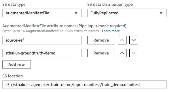
For the Input data configuration, leave the Channel name as train, for Content type put csv, Compression type as None, Record wrapper as None, S3 data type as S3Prefix, and S3 data distribution type as FullyReplicated. Finally, your S3 location should be s3://<your-bucket-name>/output/train .

Select Add channel, and repeat this input for the validation set. Set the Channel name as validation, for Content type put csv, Compression type as None, Record wrapper as None, S3 data type as S3Prefix, and S3 data distribution type as FullyReplicated. Finally, your S3 location should be s3://<your-bucket-name>/output/validation .

Finally, for the Output data configuration, set the S3 output path to s3://<your-bucket-name>/xgb.

Choose Create training job.

Alternatively, we can run this entire process in our Jupyter notebook. Run the following cell, labeled Run Amazon SageMaker XGBoost Training Job:

### Run Amazon SageMaker XGBoost Training Job

from sagemaker.amazon.amazon_estimator import get_image_uri

import random
import string

# Get XGBoost container image for current region
training_image = get_image_uri(region, 'xgboost', repo_version="latest")

# Create a unique training job name
training_job_name = 'xgboost-cars-'+''.join(random.choice(string.ascii_lowercase + string.digits) for _ in range(8))

# Create the training job in Amazon SageMaker
sagemaker = boto3.client('sagemaker')
response = sagemaker.create_training_job(
    TrainingJobName=training_job_name,
    HyperParameters={
        'early_stopping_rounds ': '5',
        'num_round': '10',
        'objective': 'multi:softmax',
        'num_class': '4',
        'eval_metric': 'mlogloss'

    },
    AlgorithmSpecification={
        'TrainingImage': training_image,
        'TrainingInputMode': 'File',
    },
    RoleArn=role,
    InputDataConfig=[
        {
            'ChannelName': 'train',
            'DataSource': {
                'S3DataSource': {
                    'S3DataType': 'S3Prefix',
                    'S3Uri': 's3://{}/output/train'.format(bucket_name),
                    'S3DataDistributionType': 'FullyReplicated'
                }
            },
            'ContentType': 'text/csv',
            'CompressionType': 'None',
            'RecordWrapperType': 'None',
            'InputMode': 'File'
        },
        {
            'ChannelName': 'validation',
            'DataSource': {
                'S3DataSource': {
                    'S3DataType': 'S3Prefix',
                    'S3Uri': 's3://{}/output/validation'.format(bucket_name),
                    'S3DataDistributionType': 'FullyReplicated'
                }
            },
            'ContentType': 'text/csv',
            'CompressionType': 'None',
            'RecordWrapperType': 'None',
            'InputMode': 'File'
        },
    ],
    OutputDataConfig={
        'S3OutputPath': 's3://{}/xgb'.format(bucket_name)
    },
    ResourceConfig={
        'InstanceType': 'ml.m4.xlarge',
        'InstanceCount': 1,
        'VolumeSizeInGB': 1
    },
    StoppingCondition={
        'MaxRuntimeInSeconds': 3600
    },)

print('{}n'.format(response))

# Monitor the status until completed
job_run_status = sagemaker.describe_training_job(TrainingJobName=training_job_name)['TrainingJobStatus']
while job_run_status not in ('Failed', 'Completed', 'Stopped'):
    job_run_status = sagemaker.describe_training_job(TrainingJobName=training_job_name)['TrainingJobStatus']
    print (job_run_status)
    time.sleep(30)

This will run our XGBoost training job in Amazon SageMaker, and monitor the progress of the job. Once the job status is ‘Completed,’ you can move on to the next cell.

This will train the model on the preprocessed data we created earlier. After a few minutes, usually less than 5, the job should be completed successfully, and it should output our model artifacts to the S3 location we specified. After this is done, we can deploy an inference pipeline that consists of pre-processing, inference, and post-processing steps.

Deploying an Amazon SageMaker endpoint using your pre-processing artifacts

Now that we have a set of model artifacts, we can set up an inference pipeline that executes sequentially in Amazon SageMaker. We start by setting up a model, which will point to all of our model artifacts, then we setup an endpoint configuration to specify our hardware, and finally we can stand up an endpoint. With this endpoint, we will pass the raw data and no longer need to write pre-processing logic in our application code. The same pre-processing steps that ran for training can be applied to inference input data for better consistency and ease of management.

From the Amazon SageMaker console, select Models choose Inference options on the left. Choose Create model. This will bring you to the model settings. For the Model name, put pipeline-xgboost. For the IAM role, select the SageMaker execution role you created earlier for your Notebook instance. It should look like this:

For Container definition 1, under Container input options, choose Provide model artifacts and inference image location. Under Location of inference image enter 246618743249.dkr.ecr.us-west-2.amazonaws.com/sagemaker-sparkml-serving:2.2. This is the SparkML serving image provided by Amazon SageMaker. The full list of SparkML images provided for every region is available here. Under Location of model artifacts, enter s3://<your-bucket-name>/model/model.tar.gz. These are the pre-processor artifacts created when running the AWS Glue job we ran earlier.

Next, we need to define a schema for our SparkML serving container via an Environment variable. For the Key enter SAGEMAKER_SPARKML_SCHEMA, and for Value enter:

{"input":[{"type":"string","name":"buying"},{"type":"string","name":"maint"},{"type":"string","name":"doors"},{"type":"string","name":"persons"},{"type":"string","name":"lug_boot"},{"type":"string","name":"safety"}],"output":{"type":"double","name":"features","struct":"vector"}}

Select Add container.

For Container definition 2, under Container input options, select Provide model artifacts and inference image location.

Under Location of inference image enter 433757028032.dkr.ecr.us-west-2.amazonaws.com/xgboost:latest. This is the XGBoost serving container provided by Amazon SageMaker. Under Location of model artifacts, enter s3://<your-bucket-name>/xgb/xgb/output/model.tar.gz. This archive contains the serialized XGBoost model artifacts from our earlier training job.

No Environment variables are needed for Container definition 2.

Choose Add container.

Finally, for Container definition 3, under Container input options, select Provide model artifacts and inference image location. Under Location of inference image enter 246618743249.dkr.ecr.us-west-2.amazonaws.com/sagemaker-sparkml-serving:2.2. This is the same SparkML serving image provided by Amazon SageMaker that we used for Container definition 1. Under Location of model artifacts, enter s3://<your-bucket-name>/model/postprocess.tar.gz. This is the reverse indexer that allows us to go from the indexed value output by XGBoost back to the original label.

Next we need to define a schema for our SparkML serving container using an Environment variable. For the Key enter SAGEMAKER_SPARKML_SCHEMA, and for Value enter:

{"input": [{"type": "double", "name": "label"}], "output": {"type": "string", "name": "cat"}}

After all three container definitions are in place, choose Create model.

You can now find your models underneath Inference, Models in the Amazon SageMaker console. Select the pipeline-xgboost model from the list to bring up the model details. Now choose the Create endpoint button.

Under Endpoint, Endpoint name, input pipeline-xgboost.

Under New endpoint configuration provide the Endpoint configuration name of pipeline-xgboost. Choose Create endpoint configuration.

Finally, choose Create endpoint at the bottom.

Alternatively, all of these steps can be run in the notebook by running the cell labeled Create SageMaker endpoint with pipeline:

### Create SageMaker endpoint with pipeline
from botocore.exceptions import ClientError

# Image locations are published at: https://github.com/aws/sagemaker-sparkml-serving-container
sparkml_images = {
    'us-west-1': '746614075791.dkr.ecr.us-west-1.amazonaws.com/sagemaker-sparkml-serving:2.2',
    'us-west-2': '246618743249.dkr.ecr.us-west-2.amazonaws.com/sagemaker-sparkml-serving:2.2',
    'us-east-1': '683313688378.dkr.ecr.us-east-1.amazonaws.com/sagemaker-sparkml-serving:2.2',
    'us-east-2': '257758044811.dkr.ecr.us-east-2.amazonaws.com/sagemaker-sparkml-serving:2.2',
    'ap-northeast-1': '354813040037.dkr.ecr.ap-northeast-1.amazonaws.com/sagemaker-sparkml-serving:2.2',
    'ap-northeast-2': '366743142698.dkr.ecr.ap-northeast-2.amazonaws.com/sagemaker-sparkml-serving:2.2',
    'ap-southeast-1': '121021644041.dkr.ecr.ap-southeast-1.amazonaws.com/sagemaker-sparkml-serving:2.2',
    'ap-southeast-2': '783357654285.dkr.ecr.ap-southeast-2.amazonaws.com/sagemaker-sparkml-serving:2.2',
    'ap-south-1': '720646828776.dkr.ecr.ap-south-1.amazonaws.com/sagemaker-sparkml-serving:2.2',
    'eu-west-1': '141502667606.dkr.ecr.eu-west-1.amazonaws.com/sagemaker-sparkml-serving:2.2',
    'eu-west-2': '764974769150.dkr.ecr.eu-west-2.amazonaws.com/sagemaker-sparkml-serving:2.2',
    'eu-central-1': '492215442770.dkr.ecr.eu-central-1.amazonaws.com/sagemaker-sparkml-serving:2.2',
    'ca-central-1': '341280168497.dkr.ecr.ca-central-1.amazonaws.com/sagemaker-sparkml-serving:2.2',
    'us-gov-west-1': '414596584902.dkr.ecr.us-gov-west-1.amazonaws.com/sagemaker-sparkml-serving:2.2'
}



try:
    sparkml_image = sparkml_images[region]

    response = sagemaker.create_model(
        ModelName='pipeline-xgboost',
        Containers=[
            {
                'Image': sparkml_image,
                'ModelDataUrl': 's3://{}/model/model.tar.gz'.format(bucket_name),
                'Environment': {
                    'SAGEMAKER_SPARKML_SCHEMA': '{"input":[{"type":"string","name":"buying"},{"type":"string","name":"maint"},{"type":"string","name":"doors"},{"type":"string","name":"persons"},{"type":"string","name":"lug_boot"},{"type":"string","name":"safety"}],"output":{"type":"double","name":"features","struct":"vector"}}'
                }
            },
            {
                'Image': training_image,
                'ModelDataUrl': 's3://{}/xgb/{}/output/model.tar.gz'.format(bucket_name, training_job_name)
            },
            {
                'Image': sparkml_image,
                'ModelDataUrl': 's3://{}/model/postprocess.tar.gz'.format(bucket_name),
                'Environment': {
                    'SAGEMAKER_SPARKML_SCHEMA': '{"input": [{"type": "double", "name": "label"}], "output": {"type": "string", "name": "cat"}}'
                }

            },
        ],
        ExecutionRoleArn=role
    )

    print('{}n'.format(response))
    
except ClientError:
    print('Model already exists, continuing...')


try:
    response = sagemaker.create_endpoint_config(
        EndpointConfigName='pipeline-xgboost',
        ProductionVariants=[
            {
                'VariantName': 'DefaultVariant',
                'ModelName': 'pipeline-xgboost',
                'InitialInstanceCount': 1,
                'InstanceType': 'ml.m4.xlarge',
            },
        ],
    )
    print('{}n'.format(response))

except ClientError:
    print('Endpoint config already exists, continuing...')


try:
    response = sagemaker.create_endpoint(
        EndpointName='pipeline-xgboost',
        EndpointConfigName='pipeline-xgboost',
    )
    print('{}n'.format(response))

except ClientError:
    print("Endpoint already exists, continuing...")


# Monitor the status until completed
endpoint_status = sagemaker.describe_endpoint(EndpointName='pipeline-xgboost')['EndpointStatus']
while endpoint_status not in ('OutOfService','InService','Failed'):
    endpoint_status = sagemaker.describe_endpoint(EndpointName='pipeline-xgboost')['EndpointStatus']
    print(endpoint_status)
    time.sleep(30)

After a few minutes, Amazon SageMaker creates an endpoint using all three of the provided containers on a single instance. When the endpoint is invoked with a payload, the output of the earlier containers is passed as the input to the later containers, until the payload reaches its final output.

In this example, the raw string categories are sent to our preprocessing MLeap container and run through a Spark pipeline to one hot encode the features. Then the one hot encoded data is sent to our XGBoost container, where our model makes a prediction to an index. The index is then fed to our post-processing MLeap container, with a Spark model artifact, which converts the index back to its original label string, which is returned to the client. These are the same steps you used for preprocessing training data, and it was only necessary to write the code once.

Testing the endpoint, monitoring, and metrics

After the Amazon SageMaker endpoint is InService, we can test it by calling the invoke-endpoint command from the AWS CLI. For example, we can use the following command:

aws sagemaker-runtime invoke-endpoint --point-name pipeline-xgboost --content-type text/csv --body low,low,5more,more,big,high out

If successful, you should see a message like this:

{
    "ContentType": "text/csv",
    "InvokedProductionVariant": "default-variant-name"
}

The output of the invocation appears in the file out, and you can see it with the following command:

cat out

If successful, this should return one of the following values: unacc, acc, good, vgood.

Alternatively, this can be done in the notebook by running the cell labeled Invoke the Endpoint:

### Invoke the Endpoint
client = boto3.client('sagemaker-runtime')

sample_payload=b'low,low,5more,more,big,high'

response = client.invoke_endpoint(
    EndpointName='pipeline-xgboost',
    Body=sample_payload,
    ContentType='text/csv'
)

print('Our result for this payload is: {}'.format(response['Body'].read().decode('ascii')))

Metrics for your inference pipelines

When building your deployments, you may find you need to monitor or debug your endpoint, and the new inference pipelines change how the logs appear in Amazon CloudWatch. You can now see logs and metrics for each of your containers within a single endpoint. To see these logs, return to the AWS Management Console, and go to Services, Amazon SageMaker, Inference, and then Endpoints. Locate your pipeline-xgboost endpoint in the list, and select it by the name to see the endpoint details.

Locate the Monitor section, and you will find a View logs link. Select it, and you will be taken to a CloudWatch Logs interface. For our example endpoint, there are three sets of log streams, one for each container. It should look like this:

If an invocation gives an error, the relevant output will appear in the relevant log stream. Whatever is output to stdout for each container will end up at this location.

Cleaning up your AWS environment

When you are done with this experiment, make sure to delete your Amazon SageMaker endpoint to avoid incurring unexpected costs. You can do this from the console by going to Services, Amazon SageMaker, Inference, and Endpoints. Choose pipeline-xgboost under Endpoints. In the upper-right, choose Delete. This will remove the endpoint from your AWS account. You will also want to make sure to stop your Notebook instance.

A more extensive cleanup can be done from your Notebook instance by running the code cell labeled Environment cleanup, as follows:

### Environment cleanup

print('Deleting SageMaker endpoint...')
result = sagemaker.delete_endpoint(
    EndpointName='pipeline-xgboost'
)
print(result)

print('Deleting SageMaker endpoint config...')
result = sagemaker.delete_endpoint_config(
    EndpointConfigName='pipeline-xgboost'
)
print(result)

print('Deleting SageMaker model...')
result = sagemaker.delete_model(
    ModelName='pipeline-xgboost'
)
print(result)

print('Deleting Glue job...')
result = glue.delete_job(
    JobName='preprocessing-cars'
)
print(result)

Conclusion

Congratulations! You have now learned how to do pre-processing and post-processing using Apache Spark in AWS Glue as part of your Amazon SageMaker ML workflow. You can now deploy a sequence of five data processing and inference steps that are executed on each inference request in Amazon SageMaker. With this new feature, you can write your pre-processing code once, and use it for both training and inference (real-time or batch). This will improve consistency between your training and deployment of your ML models. Furthermore, with the new SparkML Serving container provided by Amazon SageMaker, you can make use of Spark pipelines for real-time data. Feel free to adapt this process to different data sets or different models.

Citations

Dua, D. and Karra Taniskidou, E. (2017). UCI Machine Learning Repository. Irvine, CA: University of California, School of Information and Computer Science.

About the Authors

Thomas Hughes is a Data Scientist with AWS Professional Services. He has a PhD from UC Santa Barbara and has tackled problems in the social sciences, education, and advertising fields. He is currently working to solve some of the trickiest problems that arise when machine learning meets big data.

Urvashi Chowdhary is a Senior Product Manager for Amazon SageMaker. She is passionate about working with customers and making machine learning more accessible. In her spare time, she loves sailing, paddle boarding, and kayaking.

More than ten years ago, simpleshow started to help their customers explain materials, ideas, and products by using three-minute animated explainer videos. These explainer videos use two hands and simple, black and white illustration to lead viewers through a story. Today, the company also provides mysimpleshow.com, a platform that allows anyone to produce high-quality explainer videos about virtually any topic. This platform is integrated with Amazon Polly, so anyone can use natural sounding voices for explainer videos, as long as transcripts are provided.

First I’ll tell you a bit more about simpleshow, and then I’ll show you how mysimpleshow is integrated with Amazon Polly.

Over the past ten years, simpleshow has scientifically proven the effectiveness of the explainer video format. simpleshow experts have helped customers present their topics in a simple and entertaining way in thousands of explainer videos.

The production of these videos requires many talents in the team:

• Storytelling: Certified simpleshow concept writers create stories around basic facts.
• Illustration: Talented artists illustrate objects and concepts at the right abstraction level.
• Visualization: Storyboard artists and motion designers visualize the stories and animate them.
• Voice: A network of professional speakers ensures the right tone.

The simpleshow team realized that explainer videos are a very versatile format, so they wanted to make the resource available to even more users in even more subject areas. Therefore, the simpleshow team created mysimpleshow.com, a platform that allows anyone to produce high-quality explainer videos about virtually any topic. mysimpleshow uses artificial intelligence (AI) and has an easy-to-use user interface..

The process at mysimpleshow is very simple:

• First, users write their story. mysimpleshow provides guidance with templates and inspiration with sample stories that cover a broad selection of topics.
• The text of the story is then analyzed by the artificial intelligence at the core of mysimpleshow—the Explainer Engine. The Explainer Engine uses natural language processing (NLP) to identify meaningful keywords, people, and places. Using Wikidata, the knowledge base behind Wikipedia, keyword terms are then generalized. For example, if the name of a tennis player or basketball player is present in the story, the Explainer Engine uses Wikidata to identify the profession of the person, as a result a tennis racket or a basketball is suggested as a suitable illustration.
  
  This means that even if an illustration hasn’t been created for the person in the story, the story is visualized in a highly fitting way. For location names in the story, the Explainer Engine finds out the number of inhabitants and offers a suitable skyline as an illustration.
  
• At the click of a button, the Explainer Engine searches for the right image in the simpleshow database of all illustrations. All illustrations are tagged using a multi-tiered system.

simpleshow teams up with Amazon Polly

Spoken words are crucial for the transfer of knowledge in explainer videos. Most of the information is transmitted by voice. The illustrations and animations draw the user’s attention and support the storytelling for better understanding. As a result, the multisensory content is better retained than just a voice or animation alone.

mysimpleshow supports its users with another important component of an explainer video—it provides a computer-generated voice that reads the users’ stories. For reading the story, mysimpleshow uses Amazon Polly.

Why simpleshow uses Amazon Polly

simpleshow uses Amazon Polly for several reasons as the automated voice for explainer videos.

• mysimpleshow is an AWS-based software as a service (SaaS), making extensive use of AWS Elastic Beanstalk, Amazon DynamoDB, Amazon Simple Workflow Service (SWF), Amazon Simple Queue Service (SQS), and other AWS services. The integration of mysimpleshow and Amazon Polly was straightforward.
• With Amazon Polly, simpleshow was able to optimize the costs for text-to-speech. The team was able to significantly simplify maintenance and operations and improve scalability.
• Amazon Polly supports many languages. mysimpleshow already exists in English and German. Amazon Polly voices are available for possible extension to many other languages.
• The Amazon Polly voices are of high quality.
• Amazon Polly allows customized pronunciation of words.

All of these reasons are important, but the last one especially stood out. The Amazon Polly pronunciation lexicons enable mysimpleshow to customize the pronunciation of words.

For example, in the German language, new words are often formed by putting together existing words. Rindfleischetikettierungsüberwachungsaufgabenübertragungsgesetz (literally “beef labeling supervision duties delegation law”)[1] is a very long German compound word. Amazon Polly can handle these linguistic compounds very well on its own. However, in German, this type of word formation is also extended to words imported from other languages. For example, the name of the product—mysimpleshow— is a combination of the words my-simple-show. German-speaking users are advised to divide compounds derived from English words into the individual words. This usually significantly improves the pronunciation of these words.

Some code examples

The following code samples illustrate how mysimpleshow uses Amazon Polly.

mysimpleshow uses Simple Synthesis Markup Language (SSML) for requests to Amazon Polly. SSML gives the highest level of control over how the voices are rendered. In addition, the SSML representation is very useful for debugging purposes.

SSML

<speak><prosody volume="+20dB" rate="100%"><break time="500.0ms"/>This is Tom. He wants to buy a used car. So he starts browsing the internet.</prosody></speak>

In the first step, timings for the spoken words are requested from Amazon Polly. Timings for the keywords define when the illustration related to the keyword is placed in the scene. The spoken words basically define the timeline of the video. This is somewhat specific to Amazon Polly. Other TTS services may provide MP3 and timings together.

TTS Call Timings

import com.amazonaws.services.polly.AmazonPolly;
import com.amazonaws.services.polly.model.OutputFormat;
import com.amazonaws.services.polly.model.SynthesizeSpeechRequest;
import com.amazonaws.services.polly.model.SynthesizeSpeechResult;
import com.amazonaws.services.polly.model.TextType;
import com.mysimpleshow.backend.common.enums.Voice;
import com.mysimpleshow.backend.common.service.DictionaryService;

class TTSService {

    private DictionaryService dictionaryService;

    private AmazonPolly polly;

    public SynthesizeSpeechResult synthesizePolly(final String text, final Voice voice) {
        final SynthesizeSpeechRequest request = new SynthesizeSpeechRequest()
                .withOutputFormat(OutputFormat.Json)
                .withText(text)
                .withTextType(TextType.Ssml)
                .withVoiceId(voice.getVoiceId())
                .withLexiconNames(dictionaryService.getDictionaryNameForLocale(voice.getLocale());

        return polly.synthesizeSpeech(request);
    }
}

In the second step, the MP3 for the spoken words is generated. This is pretty much the same call as before – only the result is now MP3 instead of the JSON with the earlier timings.

TTS Call MP3

import com.amazonaws.services.polly.AmazonPolly;
import com.amazonaws.services.polly.model.OutputFormat;
import com.amazonaws.services.polly.model.SynthesizeSpeechRequest;
import com.amazonaws.services.polly.model.SynthesizeSpeechResult;
import com.amazonaws.services.polly.model.TextType;
import com.mysimpleshow.backend.common.enums.Voice;
import com.mysimpleshow.backend.common.service.DictionaryService;

class TTSService {

    private DictionaryService dictionaryService;

    private AmazonPolly polly;

    public SynthesizeSpeechResult synthesizePolly(final String text, final Voice voice) {
        final SynthesizeSpeechRequest request = new SynthesizeSpeechRequest()
            .withOutputFormat(OutputFormat.Mp3)
            .withText(text)
            .withTextType(TextType.Ssml)
            .withVoiceId(voice.getVoiceId())
            .withLexiconNames(dictionaryService.getDictionaryNameForLocale(voice.getLocale()));

        return polly.synthesizeSpeech(request);
    }
}

In the third and final step, the Amazon Polly voice, background music, more sounds, and the animation are combined into a finished video using ffmpeg.

ffmpeg -y -i <video-path> -i <sound-path> <output-path> -shortest

mysimpleshow can provide a great experience for our customers by using the variety of human voices Amazon Polly provides. In addition, using Amazon Polly is low cost; it provides an easy integration through its API; and it gives us the ability to customize voices. Amazon Polly has been a crucial AI service for mysimpleshow, and we look forward to innovating more with it.

About the Author

Hans-Christian Pahlig is Head of IT at simpleshow. He leads the development and the IT infrastructure teams. He is an internationally experienced IT expert in the media industry. As a math graduate, Hans-Christian comes from the school of thought where neural networks were conceived. If not on the job, he is inspired by the art and zen of landscape photography.

Amazon SageMaker is a complete machine learning (ML) workflow service for developing, training, and deploying models, lowering the cost of building solutions, and increasing the productivity of data science teams. Amazon SageMaker comes with many predefined algorithms. You can also create your own algorithms by supplying Docker images, a training image to train your model and an inference model to deploy to a REST endpoint.

Automating the build and deployment of machine learning models is an important step in creating production machine learning services. Models need to be retrained and deployed when code and/or data are updated. In this blog post we will discuss a technique for Amazon SageMaker automation using AWS Step Functions. We’ll demonstrate it through a new open source project, aws-sagemaker-build. This project provides a full implementation of our workflow. It includes Jupyter notebooks showing how to create, launch, stop, and track the progress of the build using Python and Amazon Alexa! The goal of aws-sagemaker-build is to provide a repository of common and useful pipelines that use Amazon SageMaker and AWS Step Functions that can be shared with the community and grown by the community.

The code is open source, and it is hosted on GitHub here.

Custom models

This blog post won’t discuss the details of how to write and design your Dockerfiles for training or inference. For more details you can dive deep into our documentation here:

• Example Project and Tutorial using aws-sagemaker-build
• Training Image Documentation
• Inference Image Documentation

What AWS services do we need?

We focus on serverless technologies and managed services to keep this solution simple. It’s important for our solution to be scalable and cost effective even when training takes a long time. Training large neural networks can sometimes take days to complete!

AWS Step Functions

There are several AWS services for workflow orchestration such as AWS CloudFormation, AWS Step Functions, AWS CodePipeline, AWS Glue and others. For our application AWS Step Functions provides the right tools to implement our workflow. Step Functions act like a state machine. They begin with an initial state and use AWS Lambda Functions to transform the state, — changing, branching, or looping through state as needed. This abstraction makes Step Functions very flexible. They also can run for up to one year and are only charged by the transition, making them a scalable and cost efficient tool for our use case.

AWS CodeBuild

AWS CodeBuild is an on demand code building service. We will use it to build our Docker images and push them to an Amazon Elastic Container Registry (Amazon ECR) repository. For more information see the documentation.

AWS Lambda

Step Functions use Lambda functions to do the work of the build. There are functions for starting training, checking on training status, starting CodeBuild, checking on CodeBuild, and so on.

One challenge was to figure out how to provide configuration parameters to different stages of the build, given that some parameters would be static, others would be dependent on previous build steps, and others would be specific to a customers need. For example, the training and inference image IDs need to be passed on to the training and deployment steps, the Amazon S3 bucket name is static to the pipeline, and the ML instances used for training and inference need to be chosen by the individual user. The solution was to also use Lambda functions. There are two Lambda functions that take as input the current state of the build and output the training job and endpoint configurations. You can edit or overwrite the code of these functions to suit your needs. For example, the Lambda function could query a data catalog to get the Amazon S3 location of a data set.

Lambdas functions are also used for various custom resources needed in setting up and tearing down the CloudFormation script. Custom resource Lambda functions include: clearing out an S3 bucket on stack delete, uploading a Jupyter notebook to the Amazon SageMaker notebook instance, clearing SageMaker resources

AWS Systems Manager Parameter Store

AWS Systems Manager Parameter Store provides a durable, centralized, and scalable data store. We will store the parameters of our training jobs and deployment here and the Step Functions’ Lambda functions will query the parameters from this store. To change the parameters you just change the JSON string in the store. The example notebooks included with aws-sagemaker-build show you how to do this.

Amazon SNS

Amazon Simple Notification service (Amazon SNS) is used for starting builds and for notifications. AWS CodeCommit, GitHub, and Amazon S3 can publish to a start-build SNS topic when a change is made. We also publish to a notifications SNS topic when the build has started, finished, and failed. You can use these topics to connect aws-sagemaker-build to other systems.

Deployment steps

To deploy an model using Amazon Sagemaker you need to do the following steps.

1. If using custom algroithms, build the Docker images and upload to Amazon ECR.
2. Create an Amazon SageMaker training job and wait to complete.
3. Create an Amazon SageMaker model.
4. Create an Amazon SageMaker endpoint configuration.
5. Create/update a SageMaker endpoint and wait for it to finish.

Those are the steps that aws-sagemaker-build will automate using Step Functions.

Achitecture

• The following diagram describes the flow of the Step Functions state machine. There are several points where the state machine has to poll and wait for a task to be completed.
  
• The following diagram shows how the services work together
  

Launch

The following CloudFormation template will create resources in your account. These include an Amazon SageMaker notebook instance and an Amazon SageMaker Endpoint, both resources you pay for by the hour.

Note: To order to prevent unnecessary charges, please tear down this stack when you are done!

Click the “Lauch Stack” button below to launch the aws-sagemaker-build CloudFormation template. Choose a name for your CloudFormation stack and leave all the other parameters at defaults.

Once your template has finished being created follow these instructions:

1. In the outputs of your stack choose the link next to NoteBookUrl
2. In the Jupyter browser choose the SageBuild folder so see the example notebooks for how to use aws-sagemaker-build.

Set up events and notifications

The CloudFormation stack can automatically create a CodeCommit repo and an S3 bucket that will launch a build when any updates happen. Do this by setting the “BucketTriggerBuild” or “BucketTriggerBuild” stack parameters to non-default values. You can have other events trigger rebuilds by publishing to the LaunchTopic SNS topic in the outputs of the CloudFormation template. To setup a GitHub repo to trigger rebuilds on changes follow the instructions in this blog post  You can also have the TrainStatusTopic send email or text you updates by subscribing it.

Alexa skill

The CloudFormation stack has an output named AlexaLambdaArn. You can use this Lambda function to create an Alexa skill to manage aws-sagemaker-build:

1. Download the model definition:json
2. The Lambda function is already configured with permissions to be called by Alexa.
3. Create an Amazon Developer account if you don’t have one. This is different than your AWS account.
4. Create the Alexa skill following these instructions:
   1. Log In to the Amazon developer console and choose the “Alexa Skills Kit” tab.
   2. In the next screen choose “custom” for your skill type and give your skill a name.
   3. In the menu on the left choose “Invocation” and give your skill an invocation name like “sagebuild”.
   4. In the menu on the left choose “Endpoint” and copy the AlexaLambdaArn output from your aws-sagemaker-build stack and paste into the default region field under “AWS Lambda Arn”
   5. In the menu on the left choose “JSON Editor” and copy the model definition you downloaded and paste in to the editor
   6. Choose “Save Model” and then “Build Model”

You can now have a workflow where you push code changes to a repository (or upload new data), make some dinner, and periodically ask Alexa, “Alexa, ask SageBuild, ‘Is my build done?’.” I have done this and it is very awesome!

Validation

aws-sagemaker-build does not do any validation on your training. This means that if your training job does not fail then the model is deployed to the endpoint, even if that model does not perform better than the current model. Your training job should contain logic to validate your model and cause the training to fail if necessary.

Frameworks

aws-sagemaker-build supports four different configurations: Bring-Your-Own-Docker (BYOD), Amazon SageMaker algorithms, TensorFlow, and MXNet. The configuration is set as a parameter of the CloudFormation template but can be changed after deployment. For the TensorFlow and MXNet configurations the user scripts are copied and saved with version names so that roll backs or redeployment of old versions works correctly. The notebook that is launched in the aws-sagemaker-build stack has examples of each different configuration.

Advanced

Dev/Prod deployments

First Create a CodeCommit repo and an Amazon S3 data bucket. Then launch two aws-sagemaker-build stacks, both using the repo and the S3 bucket you just created. Set one stack to use the “master” branch and another to use the “dev” branch.

Here is a diagram of what that architecture would look like:

Amazon CloudWatch Events

With Amazon CloudWatch Events you can publish to your stack’s LaunchTopic topic on a regular schedule (for example, everyday at 5pm or once a week on Friday at 9pm). You can use this in a workflow in which you have a smaller development dataset that you develop with during the week. You pushing your tested changes to your code branch, and you only redeploy this branch at the end of the week. This way you’re not constantly training large models and replacing them, which can be very expensive.

Conclusion and let us know what you think

If this blog post helps you or inspires you to solve a problem we would love to hear about it! We also have the code up on GitHub for you to use and extend. Contributions are always welcome!

Acknowledgements

Dua, D. and Karra Taniskidou, E. (2017). UCI Machine Learning Repository [http://archive.ics.uci.edu/ml]. Irvine, CA: University of California, School of Information and Computer Science.

About the Author

John Calhoun is a machine learning specialist for AWS Public Sector. He works with our customers and partners to provide leadership on machine learning, helping them shorten their time to value when using AWS.

In the previous blog post, we showed you how to string together Amazon Transcribe and Amazon Comprehend to be able to conduct sentiment analysis on call conversations from contact centers. Here, we demonstrate how to leverage AWS CloudFormation to automate the process and deploy your solution at scale.

Solution Architecture

The following diagram illustrates architecture that takes uses Amazon Transcribe to create text transcripts of call recordings from contact centers. In this example, we refer to Amazon Connect (cloud-based contact center service), but the architecture could work for any contact center.

The following diagram describes the architecture for processing transcribed text by using Amazon Comprehend to conduct Entity, Sentiment and Key Phrases analysis. Finally, we can visualize the analysis using a combination of Athena and QuickSight.

Automate and Deploy using AWS CloudFormation

Here, we will use AWS CloudFormation to automate and deploy the above solution.

First, login to AWS Console and Click on this link to launch the template in CloudFormation.

In the console, provide the following parameters:

• RecordingsPrefix: S3 prefix where split recordings will be stored
• TranscriptsPrefix: S3 prefix where transcribed text will be stored
• TranscriptionJobCheckWaitTime: Time in seconds to wait between transcription wait checks

Leave all other default values. Select both “I acknowledge that AWS CloudFormation might create IAM resources” checkboxes, click on “Create Change Set”, and then choose Execute.

This solution follows below steps:

1. Amazon Connect drops call recording and CTR records into Amazon S3
2. S3 Put request triggers AWS Lambda function to split call recording into two media channels – One for Agent and other for Customer. It drops two output audio files into different folders.
3. Audio drop into S3 folder triggers Lambda function to invoke AWS Step Function.
4. Step function is used here for scheduling Lambda Functions, which invokes APIs for Amazon Transcribe.
   1. Step 1 from Step Function starts Transcriptions of Audio files.
   2. Step 2 checks status of Transcription Job at regular intervals. Once job status is complete then it goes to Step 3.
   3. Step 3 – Once Transcription Job Status is complete, it writes Transcribed output into S3 Folder.
5. Transcribed text drop into S3 triggers Lambda, which invokes Amazon Comprehend APIs and writes Entity, Sentiment, Key Phrases and Language output into S3 folder. If you need to write output into Amazon Data Warehouse – Redshift then you can leverage Kinesis Firehose.
6. AWS Glue is used to maintain database catalogue and database table structure. Amazon Athena to query data out of S3 using Glue database catalogue. This completes the CloudFormation template.
7. Amazon QuickSight is used to analyze call recordings and performs sentiment, Key Phrases analysis of caller and Agent’s interactions.

Visualize Analysis using Amazon QuickSight

We can visualize Amazon Comprehend’s sentiment analysis by using Amazon QuickSight. First, we must grant Amazon QuickSight access to Amazon Athena and the associated S3 buckets in the account. For more information on doing this, see Managing Amazon QuickSight Permissions. We can then create a new data set in Amazon QuickSight based on the Athena table that was created during deployment.

After setting up permissions, we can create a new analysis in Amazon QuickSight by choosing New analysis.

Then we add a new data set.

We choose Athena as the source and give the data source a name such as connectcomprehend.

Choose the name of the database and the Use Customer SQL

Give a Name to Custom SQL such as “Sentiment_SQL” and enter below SQL. Replace Database name <YOUR DATABASE NAME> with your one.

WITH sentiment AS (
  SELECT
    contactid
    ,talker
    ,text
    ,sentiment
  FROM
    "<YOUR DATABASE NAME>"."sentiment_analysis"
)
SELECT
  contactid
  ,talker
  ,transcript
  ,sentimentresult.sentiment
  ,sentimentresult.sentimentscore.positive
  ,sentimentresult.sentimentscore.negative
  ,sentimentresult.sentimentscore.mixed
FROM
  sentiment
  CROSS JOIN UNNEST(text) as t(transcript)
  CROSS JOIN UNNEST(sentiment) as t(sentimentresult)

Choose Confirm query.

Select Import to SPICE option and then choose Visualize

After that, we should see the following screen.

Now we can create some visualizations by adding Sentiment Analysis into visualization.

Similarly, you can analyze other Comprehend output such as Entity, Key Phrases, and Language. If you have Amazon Connect CTR records available on S3 then you can blend data between comprehend output with CTR records.

Conclusion

Amazon AI services such as Amazon Transcribe and Amazon Comprehend make it easy to analyze contact center recordings by blending it with other data sources such as CTR (Call Details), Call Flow Logs, and business-specific attributes. Enterprises can reap significant benefits by realizing the hidden value in the massive amounts of caller-agent audio recordings from their contact centers. By deriving meaningful insights, enterprises can enhance both efficiency and performance of call centers and improve their overall service quality to end customers. So far, we’ve used Amazon Transcribe to transform audio data into text transcripts and then used Amazon Comprehend to run text analysis. Along the way, we’ve also used Lambda and Step Functions to string together the solution. And finally, AWS Glue, Amazon Athena, and Amazon Quicksight to visualize the analysis.

About the Authors

Deenadayaalan Thirugnanasambandam is a Senior Cloud Architect in the Professional Services team in Australia.

Piyush Patel is a big data consultant with AWS.

Paul Zhao is a Sr. Product Manager at AWS Machine Learning. He manages the Amazon Transcribe service. Outside of work, Paul is a motorcycle enthusiast and avid woodworker.

Revanth Anireddy is a professional services consultant with AWS.

Loc Trinh is a Solutions Architect for AWS Database and Analytics services. In his spare time, he captures data from his eating and fitness habits and uses analytical modeling to determine why he is still out of shape.

We’re excited to announce that Amazon Transcribe now supports automatic speech recognition in three new languages: French, Italian, and Brazilian Portuguese. These new languages expand upon the 5 languages already available in Amazon Transcribe: US English, US Spanish, Australian English, British English, and Canadian French.

Using the Amazon Transcribe API, you can analyze audio files stored in Amazon S3 and have the service return a text file of the transcribed speech. You can also send a live audio stream to Amazon Transcribe and receive a stream of transcripts in real time. Automatic transcription is proving to be an extremely useful tool for many developers, across many domains (such as subtitles for videos, contact center call analytics and compliance, court depositions, and generally improving accessibility to any application).

You can learn more about how to use transcription in contact centers (including Amazon Connect) from this recent re:Invent breakout session:

French, Italian, and Brazilian Portuguese transcription is available at the same price, and in the same Regions, as other languages in Amazon Transcribe. You can try the new set of languages through the AWS Management Console, the AWS Command Line Interface, and the AWS SDKs.

About the Author

Paul Zhao is a Sr. Product Manager at AWS Machine Learning. He manages the Amazon Transcribe service. Outside of work, Paul is a motorcycle enthusiast and avid woodworker.

Amazon SageMaker now comes pre-configured with the Scikit-Learn machine learning library in a Docker container. Scikit-Learn is popular choice for data scientists and developers because it provides efficient tools for data analysis and high quality implementations of popular machine learning algorithms through a consistent Python interface and well documented APIs. Scikit-Learn executes quickly and can scale to most data sets and problems, making it an ideal choice when you need to iterate quickly on your machine learning problems. Unlike Deep Learning frameworks such as TensorFlow or MxNet, Scikit-Learn is used for machine learning and data analysis. You can select from a range of supervised and unsupervised learning algorithms for clustering, regression, classification, dimensionality reduction, feature preprocessing, and model selection.

The newly added Scikit-Learn library is available in the Amazon SageMaker Python SDK. You can write your Scikit-Learn script and use the Amazon SageMaker training capabilities, including automatic model tuning. Once your model is trained, you can deploy your Scikit-Learn models to highly available endpoints that auto-scale to make real-time predictions with low latency. You can also use the same models in large-scale batch transform jobs.

In this blog post, I show you how to use the pre-built Scikit-Learn library in Amazon SageMaker to build, train, and deploy a multi-class classification model.

Training and deploying a Scikit-Learn model

In this example, we’re going to train a decision tree classifier on the IRIS dataset. This example is based on the Scikit-Learn Decision Tree Classification example. The full Amazon SageMaker notebook is available to try out. We’ll highlight the most important pieces here. This dataset has 50 samples from three different species of Iris flower, and is commonly used to demonstrate machine learning techniques. The goal is to predict which of the three species a flower belongs to, based on a number of different properties (petal length, petal width, and so on). While we’re using decision trees to solve this problem, Scikit-Learn offers a number of other algorithms that you can use.

Entry point script

The first step is to write the Scikit-Learn script. Starting with the main guard, we use a parser to read the hyperparameters that we pass to our Amazon SageMaker Estimator when creating the training job. These hyperparameters are made available as arguments to our input script in the training container. In this example, we look for the maximum number of leaf nodes. We also parse a number of Amazon SageMaker-specific environment variables to get information about the training environment, such as the location of input data and location where we want to save the model.

if __name__ == '__main__':
    parser = argparse.ArgumentParser()

    # Hyperparameters are described here. In this simple example we are just including one hyperparameter.
    parser.add_argument('--max_leaf_nodes', type=int, default=-1)

    # SageMaker specific arguments. Defaults are set in the environment variables.
    parser.add_argument('--output-data-dir', type=str, default=os.environ['SM_OUTPUT_DATA_DIR'])
    parser.add_argument('--model-dir', type=str, default=os.environ['SM_MODEL_DIR'])
    parser.add_argument('--train', type=str, default=os.environ['SM_CHANNEL_TRAIN'])

    args = parser.parse_args()

After we’ve defined our hyperparameters, we then load the dataset. For this example, we load all of the CSV files using the Pandas library.

    # Take the set of files and read them all into a single pandas dataframe
    input_files = [ os.path.join(args.train, file) for file in os.listdir(args.train) ]
    if len(input_files) == 0:
        raise ValueError(('There are no files in {}.n' +
                          'This usually indicates that the channel ({}) was incorrectly specified,n' +
                          'the data specification in S3 was incorrectly specified or the role specifiedn' +
                          'does not have permission to access the data.').format(args.train, "train"))
    raw_data = [ pd.read_csv(file, header=None, engine="python") for file in input_files ]
    train_data = pd.concat(raw_data)

In this example, we assume that the label (which species the flower belongs to) is stored in the first column. We separate our features and the label into two separate data frames.

    # labels are in the first column
    train_y = train_data.ix[:,0]
    train_X = train_data.ix[:,1:]

Now we’re ready to train our model. This is as simple as creating the right classifier and calling fit. A key benefit of Scikit-Learn is the simplicity and consistency of the interface that each algorithm exposes. If your model needs pre-processing of features or calculation of validation scoresc, you can also do those things in this step.

    # We determine the number of leaf nodes using the hyper-parameter above.
    max_leaf_nodes = args.max_leaf_nodes

    # Now use scikit-learn's decision tree classifier to train the model.
    clf = tree.DecisionTreeClassifier(max_leaf_nodes=max_leaf_nodes)
    clf = clf.fit(train_X, train_y)

Finally, we save our model.

    # Save the decision tree model.
    joblib.dump(clf, os.path.join(args.model_dir, "model.joblib"))

Amazon SageMaker notebook – Setup

Now that we’ve written our Scikit-Learn script we can run it on Amazon SageMaker using the Amazon SageMaker pre-built Scikit-Learn container. We’re going to use a hosted Jupyter notebook to orchestrate the training process. Feel free to follow along interactively by running the notebook.

First, we set up the Amazon S3 bucket for storing the data and the model, as well as the AWS Identity and Access Management (IAM) role for the data and Amazon SageMaker permissions.

import sagemaker

# S3 prefix
prefix = 'scikit-iris'

# Get a SageMaker-compatible role used by this Notebook Instance.
role = sagemaker.get_execution_role()

Now we’ll import the Python libraries we’ll need and create an Amazon SageMaker session.

from sagemaker.sklearn.estimator import SKLearn

sagemaker_session = sagemaker.Session()

Next, we’ll download our dataset and upload it to Amazon S3. In this example, we use Scikit-Learn locally in our notebook since it provides convenience functions to download the IRIS dataset.

import numpy as np
import os
from sklearn import datasets

# Load Iris dataset, then join labels and features together
iris = datasets.load_iris()
joined_iris = np.insert(iris.data, 0, iris.target, axis=1)


# Create a temporary directory and write the dataset as CSV
os.makedirs('./data', exist_ok=True)
np.savetxt('./data/iris.csv', joined_iris, delimiter=',', fmt='%1.1f, %1.3f, %1.3f, %1.3f, %1.3f')

# Upload the dataset to S3.
train_input = sagemaker_session.upload_data('data', key_prefix="{}/{}".format(prefix, 'data'))

Amazon SageMaker notebook – Training

Now that we’ve prepared the training data and our Scikit-Learn script (which we’ll name scikit_learn_iris.py), the SKLearn class in the SageMaker Python SDK allows us to run that script as a training job on the Amazon SageMaker managed training infrastructure. We’ll also pass the estimator our IAM role, the type of instance we want to use, and a dictionary of the hyperparameters that we want to pass to our script. Since Scikit-Learn runs on a single CPU-only machine, the Estimator only supports an instance count for training of 1 and GPU instances are not supported.

sklearn = SKLearn(
    entry_point='scikit_learn_iris.py',
    train_instance_type="ml.c4.xlarge",
    role=role,
    sagemaker_session=sagemaker_session,
    hyperparameters={'max_leaf_nodes': 30})

After we’ve constructed our SKLearn estimator, we can fit it by passing in the data we uploaded to Amazon S3. Amazon SageMaker makes sure our data is available in the local filesystem of the training cluster, so our Scikit-Learn script can simply read the data from disk.

sklearn.fit({'train': train_input})

Amazon SageMaker Notebook – Deployment

After training, we can use the SKLearn estimator to create an Amazon SageMaker endpoint – a hosted and managed prediction service that we can use to perform inference.

To do this our scikit_learn_iris.py script needs a model_fn() function that loads our saved model to make predictions.

def model_fn(model_dir):
    clf = joblib.load(os.path.join(model_dir, "model.joblib"))
    return clf

You can also optionally specify other functions to customize the behavior of deserialization of the input request (input_fn()), serialization of the predictions (output_fn()), and how predictions are made (predict_fn()). The defaults work for our current use-case so we don’t need to define them.

For more details on the default implementations to customize the behavior, see the SageMaker Scikit-Learn Container GitHub Repository.

Now we can use our SKLearn estimator in the notebook to deploy the model. The deploy() function allows us to set the number and type of instances that will be used for the prediction endpoint. These do not need to be the same values we used for the training job. Here we will deploy the model to a single ml.m4.xlarge instance but you can also deploy the model to more than one instance and set up Auto Scaling for the endpoint.

predictor = sklearn.deploy(initial_instance_count=1, instance_type="ml.m4.xlarge")

Amazon SageMaker notebook – Prediction and evaluation

Now we can use this predictor to classify flowers from the IRIS dataset. Ideally, the evaluation dataset should be different from the training dataset but for this example, we’ll just reuse some of the training dataset to invoke the endpoint. .

First, we create a test dataset.

import itertools
import pandas as pd

shape = pd.read_csv("data/iris.csv", header=None)

a = [50*i for i in range(3)]
b = [40+i for i in range(10)]
indices = [i+j for i,j in itertools.product(a,b)]

test_data = shape.iloc[indices[:-1]]
test_X = test_data.iloc[:,1:]
test_y = test_data.iloc[:,0]

Now we can use the endpoint to make predictions by calling the predict function with our features.

predictor.predict(test_X.values)

Amazon SageMaker notebook – Cleanup

After you have finished with this example, remember to delete the prediction endpoint to release the instances associated with it.

sklearn.delete_endpoint()

Amazon SageMaker notebook – Batch Transform

Amazon SageMaker also provides Batch Transform, a managed service for doing large-scale that can be used to perform inference against your trained model on a large dataset. It’s ideal for scenarios where you’re dealing with large batches of data, you don’t need sub-second latency, or you need to preprocess and transform the training data.

First, we create a transformer and specify the number and type of instances we want to use for the job. In this case we specify 2 instances but you can scale this with the size of your dataset to reduce the amount of time it takes.

# Define a SKLearn Transformer from the trained SKLearn Estimator
transformer = sklearn.transformer(instance_count=2, instance_type='ml.m4.xlarge')

Now we start the transform job by providing it the location of our data on Amazon S3. The notebook example includes the steps followed to upload the dataset.

# Start a transform job and wait for it to finish
transformer.transform(batch_input_s3, content_type='text/csv')
print('Waiting for transform job: ' + transformer.latest_transform_job.job_name)
transformer.wait()

After the transform job has completed, we can download the output data from Amazon S3. For every input file we had, we will have a corresponding output file.

# Download the output data from S3 to local filesystem
batch_output = transformer.output_path
!mkdir -p batch_output
!aws s3 cp --recursive $batch_output/ batch_data/

Conclusion

In this blog post we show you how to use the Amazon SageMaker built-in Scikit-Learn container to train a model on the IRIS dataset. However, that’s just the beginning. Scikit-Learn has a large selection of algorithms and transformers that you can use for your machine learning use-cases. Amazon SageMaker enables you to use Scikit-Learn scripts and works seamlessly with SageMaker training, automatic model tuning, and deployment capabilities.

Citations

Dua, D. and Karra Taniskidou, E. (2017). UCI Machine Learning Repository

[http://archive.ics.uci.edu/ml]. Irvine, CA: University of California, School of Information and Computer Science.

About the Author

 Laurence Rouesnel is the Algorithms & Platforms Group Manager in Amazon AI Labs. He leads a team of engineers and scientists working on deep learning and machine learning research and products. In his spare time he is an avid traveler, and loves the outdoors whether it’s hiking, skiing, or windsurfing.

Eric Kim is an engineer in the Algorithms & Platforms Group of Amazon AI Labs. He helps support the AWS service SageMaker, and has experience in machine learning research, development, and application. Outside of work, he is an avid music lover and a fan of all dogs.

The success of an ecommerce platform heavily relies on the reputation that has been established through thousands of user reviews and social shares by customers. By reviewing and sharing information existing customers establish a trust relationship with something they can’t physically touch. For this content to be accessible to a global audience it’s critical to translate it into the local language to help customers make their buying decisions.

Imagine that a company that sells older cars, boats, and motorcycles has the following problem: they are expanding their ecommerce business to several countries and they want to allow their customers to effortlessly read all reviews of their offerings written by other shoppers.

To solve this problem, we’ll show you how the company can leverage Amazon Translate to get on-demand translated reviews in real time. We’ll also show you how easily they ca integrate the service in a modern ecommerce architecture.

Amazon Translate is a high-quality neural machine translation service that uses advanced deep learning techniques to provide fast language translation of content from a source language to a target language, chosen among the supported pairs. It enables developers to easily invoke an API providing the text to be translated and obtain its translated version in real-time, hiding the complexity of building a neural machine translation model.

The ecommerce architecture

Our example website is a JavaScript single-page application that is hosted in a public Amazon S3 bucket where static website hosting has been enabled.

The example company wants to extend their global presence, so they have decided to use Amazon CloudFront to speed-up the distribution of their static web content worldwide. With CloudFront, files are delivered to end  users using a global network of edge locations that reduce latency and increase data transfer rates.

The website integrates with Login with Amazon and Amazon Cognito User Pools for user authentication and authorization, and makes REST API calls to an API deployed through Amazon API Gateway.

When API resources are requested, API Gateway invokes AWS Lambda functions that implement business logic operations like listing products, getting product details, adding user reviews, and translating user reviews.

More specifically ,the Lambda function code interacts with:

• Amazon Translate, to get translated reviews
• Amazon DynamoDB, to cache translated reviews in a fast and flexible NoSQL database and avoid invoking the Translate API for reviews that had already been translated
• Amazon Comprehend, to analyse the sentiment of the reviews
• Amazon Kinesis Data Firehose, to capture translation and sentiment analysis data into Amazon S3 for further analysis
• Amazon RDS for Aurora, to store product and review data

Translating reviews and detecting language and sentiment

Wherever a user wants to translate a review, the website will make an API call to Amazon API Gateway that will execute a Lambda function that makes an API call to Amazon Translate. As you can see from the following code snippet you can see how easily you can make this call in Python by using the AWS SDK.

try:
       # Translate text
       result = translate_client.translate_text(Text=review, SourceLanguageCode=source_language, TargetLanguageCode=target_language)
       logger.info("Translation result: " +str(result))
except Exception as e:
       logger.error(str(e))
       raise e

The API call translate_text() needs only three parameters: text (in this case the review), source language (original language of the review), and target_language (the language into which you want to translate the review).

Obviously when a user writes a review we do not know which language the review is written in. The API call to post a new review will call the Lambda function PostReview. PostReview understands which language the review was written in by using Amazon Comprehendbefore saving it Amazon RDS for Aurora. Amazon Comprehend is a natural language processing (NLP) service that uses machine learning to understand the language. Amazon Comprehend is also very simple to invoke. Here the snippet of the code:

try:
       # Amazon Comprehend
       language = comprehend.detect_dominant_language(Text = review)
       logger.info("Language return: " + str(language))
except Exception as e:
       logger.error(str(e))
       raise e

When a review is posted, the Lambda function will also detect the sentiment that translate in an emoticon in the example website. To understand the sentiment of the review is also a single line of code:

try:
             # Amazon Comprehend
             sentiment = comprehend.detect_sentiment(Text=review, LanguageCode=language)
             logger.info("Sentiment ->: " + str(sentiment))
except Exception as e:
             logger.error(str(e))
             raise e

As you can see, both Amazon Comprehend detect_dominant_language() and detect_sentiment() API calls will just need the text as parameter.

Summary

Now that you’ve seen an example of how you can use Amazon Translate and Amazon Comprehend to empower your website, we hope you are inspired to create your own solutions.

Amazon Translate can get translations of a full sentence within a few milliseconds, enabling usage in both synchronous on-demand translations and in asynchronous tasks for executing a large number of translations with the aim of storing first and then delivering them.

Amazon Translate, Amazon Comprehend, Amazon Kinesis Data Firehose, Amazon S3, Amazon RDS, Amazon DynamoDB, Amazon Route 53, Amazon S3, Amazon CloudFront, Amazon API Gateway, Amazon Cognito are powerful services that allow you to implement fully-managed and serverless solutions for your business needs: the possible use cases are only limited by your imagination.

About the Authors

Giuseppe Angelo Porcelli is a Sr. Solutions Architect for Amazon Web Services in Italy. With several years engineering background, he helps enterprise customers designing flexible and resilient architectures using AWS services. His field of expertise covers Artificial Intelligence and Machine Learning. In free time, Giuseppe enjoys playing football.

Diego Natali is a solutions architect for Amazon Web Services in Italy. With several years engineering background, he helps ISV and Start up customers designing flexible and resilient architectures using AWS services. In his spare time he enjoys watching movies and riding his dirt bike.

Data scientists and developers can now easily train machine learning models on datasets labeled by Amazon SageMaker Ground Truth. Amazon SageMaker Training now accepts the labeled datasets produced in augmented manifest format as input through both AWS Management Console and Amazon SageMaker Python SDK APIs.

Last month during AWS re:Invent, we launched Amazon SageMaker Ground Truth to build highly accurate training datasets with up to 70 percent savings in labeling costs by using machine learning to aid public as well as private workforces of human labelers. The labeled datasets are produced in augmented manifest file format that augments each input dataset object with additional metadata – such as labels – inline in the file. Earlier you could use only the low-level AWS SDK APIs to train models on augmented datasets. Starting today, you can now quickly and easily perform such training with few quick clicks in the Amazon SageMaker console or one-line API calls using the high-level Amazon SageMaker Python SDK.

Furthermore, the model will be trained using the Amazon SageMaker Pipe Mode, which significantly accelerates the speeds at which data is streamed from Amazon Simple Storage Service (S3) into Amazon SageMaker so that your training job starts sooner, finishes quicker, and needs less disk space, thus reducing your overall cost to train machine learning models on Amazon SageMaker.

Now let’s dive into an example. Our example uses the CBCL StreetScenes dataset consisting of 3548 street images. In an earlier blog post we had shown you an example of how you can use Amazon SageMaker Ground Truth to manage a workforce for drawing bounding boxes around all the cars in the images, thus creating a labeled dataset for training an Amazon SageMaker Object Detection model. Now we’ll show you how to train such a model on Amazon SageMaker.

Step 1: Explore the labeled dataset

The labeled dataset is produced in an augmented manifest file format. An augmented manifest file is a file in JSON Lines format. This means that each line in the file is a complete JSON object followed by a newline separator. Each JSON object contains the Amazon S3 URI of an image file along with its labels. The labels are the coordinates of the bounding boxes around each of the cars in the image. Here is a sample JSON object from the augmented manifest file for an image that was labeled with 4 cars.

SSDB00004.JPG

Here is the JSON object in the augmented manifest file. We have formatted the display for ease of visualization. In the augmented manifest file, this will appear as a JSON object in a single line.

{
 "source-ref":"s3://sthakur/demo/images/SSDB00004.JPG",
 "sthakur-groundtruth-demo":{
   "annotations":[
     {"class_id":0,"width":162,"top":458,"height":89,"left":378},
     {"class_id":0,"width":201,"top":434,"height":96,"left":602},
     {"class_id":0,"width":61,"top":434,"height":39,"left":343},
     {"class_id":0,"width":66,"top":426,"height":47,"left":240}
   ],
   "image_size":[{"width":1280,"depth":3,"height":960}]
 },
 "sthakur-groundtruth-demo-metadata":{
   "job-name":"labeling-job/sthakur-groundtruth-demo",
   "class-map":{"0":"car"},
   "human-annotated":"yes",
   "objects":[
     {"confidence":0.09},
     {"confidence":0.09},
     {"confidence":0.09},
     {"confidence":0.09}
   ],
   "creation-date":"2018-12-13T21:24:33.546706",
   "type":"groundtruth/object-detection"
 }
}

Here source-ref is the Amazon S3 URI of the image file. Note that sthakur-groundtruth-demo (named after the Amazon SageMaker Ground Truth labeling job that produced the manifest file in the first place) is the list of labels. The labels consist of the coordinates of the four cars labeled by human labeler.

Step 2: Create the Amazon SageMaker training job

We’ll now train an Amazon SageMaker Object Detection Model which takes the augmented manifest file from Step 1 as an input.

Using the Amazon SageMaker console

Choose Training jobs from the left navigation pane on the Amazon SageMaker console and then choose Create training job. After choosing the model training configurations, such as the learning algorithm, training cluster specs, and hyperparameters, scroll down to the section where you enter the input data channel for sourcing the training dataset.

Choose the S3 data type as AugmentedManifestFile. Provide the Amazon S3 location of the manifest file from Step 1. Also provide the names of the JSON attributes that you want the Object Detection Algorithm to use from the augmented manifest file. Here we need only two attributes for training the model: source-ref and sthakur-groundtruth-demo as described in Step 1.

Since the JSON objects from the augmented manifest file are streamed in an ordered fashion using Amazon SageMaker Pipe mode, you need to carefully choose the sequence of attribute names that the algorithm should expect to find in the input data stream. Use the up and down arrow buttons next to each attribute name for choosing the sequence.

While we are showing here how to create an input data channel for sourcing training dataset, the Object Detection algorithm also requires an input data channel for validation dataset. One way to prepare the validation dataset would be to hold out a subset of your labeled images, and create another augmented manifest file for the validation set. You can then use the Amazon S3 URI of the new augmented manifest file as an input to your validation channel, and define the channel in exactly the same manner as described in this step.

Using the Amazon SageMaker Python SDK

We’ll use Amazon SageMaker Estimator to train the Object Detection Model.

od_model = sagemaker.estimator.Estimator(training_image,
                                         role, 
                                         train_instance_count=1, 
                                         train_instance_type='ml.p3.2xlarge',
                                         train_volume_size = 50,
                                         train_max_run = 360000,
                                         input_mode = 'Pipe',
                                         output_path=s3_output_location,
                                         sagemaker_session=sess)
…………………………..

train_data = sagemaker.session.s3_input(s3_train_data, distribution='FullyReplicated', content_type='image/jpeg', s3_data_type='AugmentedManifestFile', attribute_names=['source-ref', 'sthakur-groundtruth-demo'])

validation_data = sagemaker.session.s3_input(s3_validation_data, distribution='FullyReplicated', content_type='image/jpeg', s3_data_type='AugmentedManifestFile', attribute_names=['source-ref', 'sthakur-groundtruth-demo'])


…………………………………………..

data_channels = {'train': train_data, 'validation': validation_data}
od_model.fit(inputs=data_channels, logs=True)

Note that we’ve chosen the input_mode as Pipe, s3_data_type as AugmentedManifestFile, and specified the attribute_names sequence before training the model using SageMaker estimator’s fit routine.

Additional benefits of using augmented manifest format

Amazon SageMaker has always supported traditional manifest files for training models on datasets stored in Amazon S3. A manifest file simply provides a list of Amazon S3 key name prefixes for the data objects that need to be downloaded to Amazon SageMaker for training the model.

For example, this is a manifest file:

[
    {"prefix":"s3://foo/"},
  "relative/path/to/data-1",
  "relative/path/to/data-2",
  ...
]

Will match the following Amazon S3 URIs:

s3://foo/relative/path/to/data-1
s3://foo/relative/path/to/data-2

Using this traditional approach for specifying the input data channel for learning algorithms, such as visual recognition algorithms, requires you to specify two input data channels in Amazon SageMaker – one for the input data (images), and other for its labels. Using an augmented manifest, you can now put the data and its labels in one manifest file, thus reducing the need for two channels. It also eliminates any unnecessary complexity in algorithm code for matching data objects with labels across multiple channels.

For example, this manifest file can be easily expressed as an augmented manifest by restructuring the S3 URIs to JSON Lines format, and adding labels inline.

{"source-ref":"s3://foo/relative/path/to/data-1","label":"0"}
{"source-ref":"s3://foo/relative/path/to/data-2","label":"1"}
……….

Set attribute_names=['source-ref','label'] while training the model.

In addition, the augmented manifest file uses Amazon SageMaker Pipe mode, which means that your learning algorithm can benefit from the high throughput data streaming from Amazon S3 to your training instances in Amazon SageMaker. Here is a blog post that describes changes you can make to your learning algorithm to start consuming data using Pipe mode.

Get started with more examples and developer support

We’ve shown you examples of how to train models on Amazon SageMaker using labeled datasets in augmented manifest file format. You can also try out our sample notebook that provides the step-by-step AWS SDK experience. You can also see additional examples in our developer guide or post your questions on our developer forum.

About the Author

Sumit Thakur is a Senior Product Manager for AWS Machine Learning Platforms where he loves working on products that make it easy for customers to get started with machine learning on cloud. He is product manager for Amazon SageMaker and AWS Deep Learning AMI. In his spare time, he likes connecting with nature and watching sci-fi TV series.