
Blog

Learn About Our Meetup

5000+ Members

MEETUPS

LEARN, CONNECT, SHARE

Join our meetup, learn, connect, share, and get to know your Toronto AI community. 

JOB POSTINGS

INDEED POSTINGS

Browse through the latest deep learning, ai, machine learning postings from Indeed for the GTA.

CONTACT

CONNECT WITH US

Are you looking to sponsor space, be a speaker, or volunteer, feel free to give us a shout.

Category: Global

At GTC DC, Experts Describe Why Diversity in AI Makes a World of Difference

When Megan Gray, CEO of Moment AI, first tested one of her company’s services — a tool using AI to determine facial signs indicating a driver may have fallen asleep or suffered a medical issue — it didn’t work.

“The technology worked on our CTO, who is a white male. But then I tried it, and it couldn’t detect that my eyes were closed,” Gray said. “It didn’t work on me as an African-American woman.” This is just one example of how a lack of diversity in the field of AI affects the technologies that are created.

At GTC DC, this week’s Washington edition of the GPU Technology Conference, a range of events focused on sharing ideas on how workplaces can become more inclusive, and how researchers can improve their AI technology to avoid bias.

One of Forbes’ top conferences for women in tech, this year’s GTC DC was the most diverse yet. Over 20 percent of its 3,500 attendees were women.

The conference also featured an inaugural reception celebrating attendees from historically black colleges and universities and the Black in AI and LatinX in AI community groups.

As he opened the reception, Kevyn Orr, partner-in-charge at Jones Day, said, “You are the first generation that has the opportunity to make sure that development, that research and that algorithms are appropriately inclusive.”

‘Who’s Like Me?’: Finding Diverse Role Models

Catherine Ordun, senior data scientist at Booz Allen Hamilton, delivered the keynote at the GTC DC Women’s Early Career Accelerator.

GTC DC kicked off with the Women’s Early Career Accelerator, a day-long, invitation-only training and networking event attended by nearly 60 graduate students and early-career professionals.

Catherine Ordun, a senior data scientist at Booz Allen who presented the keynote at the accelerator, was honest about the challenges of being a woman in the field of AI.

“You’ll find yourself asking, ‘Who’s like me?’ And the truth is, there’s not a lot. Only 12 percent of people who do AI are women,” said Ordun, referencing a WIRED survey.

Events like the accelerator are helping to change that. After Ordun’s address, participants spent the day completing the NVIDIA Deep Learning Institute’sFundamentals of Deep Learning for Computer Vision” workshop, taught by Alex Qi, an enterprise solutions architect at NVIDIA.

The Women in AI Breakfast featured an AI ethics panel, with speakers (from left) Svetlana Matt, Emily Tait, Megan Gray and Tiffany Moore.

GTC DC also featured the third annual Women in AI Breakfast, hosted by Dell Technologies. Over quiche and coffee, a panel of experts in research, law and more discussed AI ethics.

Emily Tait, an intellectual property partner at Jones Day, provided a legal perspective on how companies can counter issues like the one Gray described. “The best companies are creating dedicated personnel and policies and cultures around diversity.” From there, they’re able to come up with more robust algorithms and identify biases in their technology.

And nearly 75 people filled out the eighth floor of the Ronald Reagan Building and International Trade Center to attend the Black and Latinx Communities Reception, sponsored by Jones Day.

The reception recognized the 50 students that were selected from historically black colleges and universities, Black in AI and LatinX in AI. They received full passes to DLI courses and the entirety of GTC DC.

Addressing a Changing Workforce

Andrew Ko, managing director for global education at AWS, spoke at the Workforce of the Future panel.

NVIDIA Senior Director of Corporate Social Responsibility Tonie Hansen moderated a panel of executives from government, nonprofits and business. They shared examples of how educational institutions, trade associations and companies can help employees prepare for modern jobs that incorporate AI and data science.

Andrew Ko, the managing director for global education at AWS, provided a corporate perspective and gave examples of career programs implemented by Amazon that help employees reskill.

Another panelist was former chief of staff for U.S. Representative Alma Adams and founder of diversity innovation house HBCU House Rhonda Foxx. She gave insight on how the federal government can help support HBCUs — historically black colleges and universities — which produce 47 percent of all black women engineers.

“With emerging technology and AI, we are on the precipice of the fourth revolution,” she said. “We all need to lean in right now and make sure there’s diversity of thought at the table as we move forward in these technological advances.”

The post At GTC DC, Experts Describe Why Diversity in AI Makes a World of Difference appeared first on The Official NVIDIA Blog.

AWS DeepRacer League: The Championship lineup is complete, making for an exciting re:Invent 2019 final!

The AWS DeepRacer League is the world’s first autonomous racing league, open to anyone. Announced at re:Invent 2018, it puts machine learning in the hands of every developer in a fun and exciting way. Since March 2019, thousands of developers of all skill levels have competed for the chance to advance to the Championship Cup at re:Invent 2019.

2019 League wrap-up

As well as racing at AWS Summits around the world, participants have been racing virtually via the AWS DeepRacer console. Developers have been testing their skills on different tracks in simulation throughout the year, and competing in monthly competitions with the hope of winning an expenses-paid trip to re:Invent 2019. The final Virtual Circuit race concluded on October 31, completing the Championship Cup lineup.

Two champions were named: the winner of the final virtual race of the year, as well as 18 top point scorers who have been competing in multiple races throughout the year. “Eric” from Taiwan won the Toronto Turnpike race with a lap time of 7.172 seconds, which is the fastest time recorded on any of the virtual tracks, and beats the world record set at the Summits. The next challenge for Eric is transitioning his models from simulation to the real world when he gets to Las Vegas!

Lyndon Leggate, an early AWS DeepRacer enthusiast and the founder of the AWS DeepRacer Slack community, was victorious in the overall virtual leaderboard and is joined by 17 other skilled racers from the Virtual Circuit. Each of the 18 racers competed in all six virtual races, racking up points along the way with very consistent models, and clocking times ranging between 9.4–14.6 seconds. We will see each of these developers at re:Invent 2019, when the in-person and virtual worlds collide in the Championship Cup knock-out rounds.

The AWS DeepRacer 2019 Summit Circuit results

The AWS DeepRacer Virtual Circuit results

Get ready to race at re:Invent

re:Invent 2019 is the final destination on the journey to crown the 2019 AWS DeepRacer Championship Cup winner. The November Championship Cup warm-up race is now open. On the newly revealed track shape, developers can train models on the official track to be used during the Championship Cup! You can take part in this friendly warm-up race via the AWS DeepRacer console and compete for up to $500 in AWS credits. See how your model performs on the official Championship Cup track today, and bring that model with you to re:Invent and race at the MGM Grand Garden Arena. There will be prizes up for grabs, all while getting a trackside seat to witness the best racers from around the world compete in the knock-outs.

The Championship Cup

The Championship Cup competition includes a set of elimination rounds at the MGM Grand Garden Arena, where 64 of the League’s best face off in a knock-out tournament in the hopes of taking home the glory! Starting on Tuesday, December 3, the field will whittle down from 64 to 3, who will go on to compete onstage in the Grand Final at Werner Vogel’s keynote on Thursday, December 5. The League will hold one final chance for in-person racers to advance to the knock-out rounds on Monday, December 2, from 4–7 PM, at the Quad in the Aria hotel. Open to all re:Invent attendees, you can race on the iconic 2019 track for a chance to advance to the finals where not one but three contestants will go through!

Learn and grow

New racers not competing for the 2019 cup can attend one of the 10 AWS DeepRacer workshops to learn how to build the best model to compete in the 2020 League and learn from AWS DeepRacer experts.

The AWS DeepRacer workshops provide customers with hands-on training, enabling them to build their models and learn more about what’s next for AWS DeepRacer. The sessions are open for registration now, so don’t miss out on your chance to learn and get ready to race!

AWS customers who want to learn and prepare for the 2020 season will benefit from the AWS DeepRacer Expert Boot Camp. This two-day event offers unprecedented access to AWS DeepRacer experts, including AWS DeepRacer data scientists, 2019 AWS Summit winners, and developer experts sharing best practices and racing tips. With a full track for practicing in real time, this is one event you do not want to miss.

The home stretch of 2019!

In less than a year, AWS DeepRacer has seen a dramatic evolution in the speeds developers are clocking on the tracks, from Rick Fish’s championship-winning time of 51.50 seconds to the world record of 7.44 seconds set by SOLA at the Tokyo Summit in June. Developers around the world have embraced the challenge, testing their models for days and weeks at a time, playing with speed and other parameters to push the car to its physical (and virtual) limits. The Championship Cup is set to be the most exciting yet. Register for re:Invent 2019 today, and start training your models to win prizes in the warm-up challenge!


About the Author

Alexandra Bush is a Senior Product Marketing Manager for AWS AI. She is passionate about how technology impacts the world around us and enjoys being able to help make it accessible to all. Out of the office she loves to run, travel and stay active in the outdoors with family and friends.


Less stress, less time: How a Brazilian startup is using Azure AI to make car repairs easier

SÃO PAOLO, Brazil For most people, the worst part of getting into a minor car accident is figuring out how to get your car repaired.

There’s the trouble of figuring out who to call, the hassle of driving around to get estimates and the constant worry that whoever you work with will end up taking advantage of you.

That’s where Car10 comes in. The Brazilian startup has created an app that allows customers to take a picture of the damage, submit the photo and get three to five estimates from nearby car repair shops that Car10 has pre-screened for quality and reliability. The startup even guarantees it will make the repair for free if you aren’t satisfied.

“We take the fear out of the process, the worry that you’ll be taken advantage of,” said Jose Tafner, Car10’s chief financial officer.

Now, the São Paolo-based company is using artificial intelligence to make the process faster. The startup announced that it is using Microsoft’s Azure Cognitive Services Custom Vision Service to almost immediately give the user a rough sense of what they expect the repair to cost.

With the current system, users who submit a photo will get a quote within 30 minutes to an hour. With the new AI tools, Tafner said they can get a general sense of how much the repair will cost within about 30 seconds.

“It goes back to the customer need. When you have a small accident or crash, the thing you want to know is how much it’s going to cost,” Tafner said. “The first need is speed and some level of accuracy.”

The AI system uses a machine learning model to compare the damage to the customer’s car with other examples of similar damage to come up with a reasonably close estimate. Then, the company works with car repair shops to get firmer bids.

The AI system may speed up the quote process, but it doesn’t replace the hands-on involvement that Car10 has in ensuring customers feel comfortable throughout the process of getting their car repaired.

Tafner said Car10 works with customers on everything from providing the estimate to scheduling the visit and even paying through Car10’s digital platform. The customer then has the opportunity to rate the experience and the shop where the repair was made.

“The digital part of the journey is small. The largest part is analog,” Tafner said.

Focus on quality

Car10 has about 100,000 customers and works with about 4,000 auto body shops throughout Brazil, ranging from big businesses to small mom-and-pop shops. Tafner said the company initially focused only on larger shops, thinking that was what the customer would prefer. But they found that customers didn’t care whether the shop was being run out of someone’s garage or a fancy office.

“They care about the quality of the service,” he said.

Car10 was started in 2014 by three brothers who had previously worked for their father’s insurance adjustment business. When that business was sold, they decided to use their experience in the car repair industry to plunge into the startup world. Tafner joined a couple of years later, after decades of global experience in the corporate world. The service is designed for people who are paying for repairs themselves, instead of relying on insurance.

From the beginning, the four-person leadership team has been highly reliant on technology and data. They run on Microsoft’s Azure cloud service, use Power BI dashboards and built the app on the .NET framework.

“The four of us are data freaks. We’re constantly using it to improve the business,” Tafner said.

Still, Tafner said that like many businesses swimming in data, it can be challenging to figure out which pieces of data are useful.

One clear winner: The photos of car repairs. Car10 was able to use that data to train the machine learning model to automatically detect what kind of repair a person needs and what it would generally cost. Car10 doesn’t sell customer data, and it protects people’s personal information using Azure security protections.

Car10, which has received startup investment funds from Microsoft, first started building the AI solution when the company participated in an industry hackfest. Although it has an IT staff, none of the people who work for Car10 have a particular expertise in AI. Azure Cognitive Services are designed so that even people without any formal AI training can use them.

Future plans

Car10 is about five years old now, and it expects to break even within a quarter. Now, Tafner said the company is seeking more funding so that it can expand into other areas of business, and potentially other markets outside of Brazil.

“What we can do for car crashes we can do for a number of things,” he said.

For Tafner, the small team and fast pace is both invigorating and enlightening. Like any startup, he notes, the company is constantly trying new things, making mistakes and adjusting – all while trying to run the core business. He likens it to race car driving.

“We’re changing the tires while the car is running,” Tafner said. “There are no pit stops for us.”

Related:

Allison Linn writes about AI and innovation. Follow her on Twitter.

The post Less stress, less time: How a Brazilian startup is using Azure AI to make car repairs easier appeared first on The AI Blog.

Highlights from the 2019 Google AI Residency Program

This fall marks the successful conclusion to the fourth year of the Google AI Residency Program. Started in 2016 with 27 individuals in Mountain View, CA, the 12-month program has grown to nearly 100 residents from nine locations across the globe. Program participants have gone on to great success in PhD programs, academia, non-profits, and industry. Many have also become full-time Google researchers.

The program’s latest installment was our most successful yet, as residents advanced progress in a broad range of research fields, such as machine perception, algorithms and optimization, language understanding, healthcare and many more. Below are a handful of innovative projects from some of this year’s alumni.

  • A large-scale study on cross-lingual transfer in massive multilingual neural machine translation models (recently highlighted as part of this post), trained on billions of sentence pairs from more than 100 languages in order to significantly improve translation for both low- and high-resource languages.
    Visualization of the clustering of encoder representations of all modeled languages, based on representational similarity. Encoder representations of different languages cluster according to linguistic similarity. Languages are color-coded by their linguistic family.
  • A generative model for Scalable Vector Graphics (SVGs), which can be used to aid designers in generating fonts.
  • Top: Unlike pixel representations of icons (right), in this case a “6”, SVGs (left; middle) are scale-invariant representations. Bottom: By modelling SVGs directly, we can aid artists in quickly and intuitively iterating over typography designs.
  • A method to learn GANs using discrepancy divergence, a measure that accounts for both the loss function and hypothesis set to provide theoretical learning guarantees.
  • As more generators are added to the DGAN ensemble more modes in the real distribution are covered. From left to right: 1 generator, 5 generators, and 10 generators.
  • A likelihood ratio method for deep generative models that effectively corrects for confounding background statistics to improve out-of-distribution (OOD) detection, and a new benchmark dataset for OOD detection in genomics.
  • Log-likelihood (left) and log likelihood-ratio (right) of each pixel for Fashion-MNIST. The likelihood is dominated by the “background” pixels, whereas the likelihood ratio focuses on the “semantic” pixels and is thus better for OOD detection.
  • A study showing when label smoothing helps, focusing on its impact on calibration of predictions, representations learned by the penultimate layer and effectiveness of knowledge distillation.
  • 2D-projection of representations of three CIFAR100 classes. Without label smoothing, examples are spread, but with label smoothing each example is encouraged to be equally distant to the clusters of the other classes, attenuating intra-class variation and inter-class similarity structure.

The successes of our AI residents go beyond academic publishing. Their achievements include:

  • Organizing a workshop, bringing together experts in theoretical physics and deep learning, to explore how tools from physics can shed light on the theory of deep learning.
  • Founding Queer in AI, an organization for fostering a community of queer researchers and raising awareness of queer issues in AI/ML.
  • Organizing a hands-on Tensorflow tutorial on using Deep Learning for Natural Language Processing.
  • Automatically learning neural net architectures with AdaNet, an open-source, TensorFlow-based framework.
  • Developing Coconet, the model behind the first AI-powered Doodle (created to celebrate renowned German composer and musician Johann Sebastian Bach).

Also, beginning with the next program cycle, residents will be hosted for a duration of 12 months, with the option of extending up to 18 months! This exciting shift comes as part of our effort to improve the overall program experience and outcomes for residents as the program continues to grow and scale.

If you are interested in joining our fifth cohort, applications for the 2020 Google AI Residency program are now open! Visit g.co/airesidency/apply for more information on how to apply. Please submit your application as soon as possible, as we will be considering candidates on a rolling basis. Please see g.co/airesidency for more resident profiles, past resident publications, blog posts and stories. We can’t wait to see where the next year will take us, and hope you’ll consider joining our research teams across the world!

Highlights from the 3rd Cohort of the Google AI Residency Program

This fall marks the successful conclusion for the third cohort of the Google AI Residency Program. Started in 2016 with 27 individuals in Mountain View, CA, the 12-month program has grown to nearly 100 residents from nine locations across the globe. Program participants have gone on to great success in PhD programs, academia, non-profits, and industry. Many have also become full-time Google researchers.

The program’s latest installment was our most successful yet, as residents advanced progress in a broad range of research fields, such as machine perception, algorithms and optimization, language understanding, healthcare and many more. Below are a handful of innovative projects from some of this year’s alumni.

  • A large-scale study on cross-lingual transfer in massive multilingual neural machine translation models (recently highlighted as part of this post), trained on billions of sentence pairs from more than 100 languages in order to significantly improve translation for both low- and high-resource languages.
    Visualization of the clustering of encoder representations of all modeled languages, based on representational similarity. Encoder representations of different languages cluster according to linguistic similarity. Languages are color-coded by their linguistic family.
  • A generative model for Scalable Vector Graphics (SVGs), which can be used to aid designers in generating fonts.
  • Top: Unlike pixel representations of icons (right), in this case a “6”, SVGs (left; middle) are scale-invariant representations. Bottom: By modelling SVGs directly, we can aid artists in quickly and intuitively iterating over typography designs.
  • A method to learn GANs using discrepancy divergence, a measure that accounts for both the loss function and hypothesis set to provide theoretical learning guarantees.
  • As more generators are added to the DGAN ensemble more modes in the real distribution are covered. From left to right: 1 generator, 5 generators, and 10 generators.
  • A likelihood ratio method for deep generative models that effectively corrects for confounding background statistics to improve out-of-distribution (OOD) detection, and a new benchmark dataset for OOD detection in genomics.
  • Log-likelihood (left) and log likelihood-ratio (right) of each pixel for Fashion-MNIST. The likelihood is dominated by the “background” pixels, whereas the likelihood ratio focuses on the “semantic” pixels and is thus better for OOD detection.
  • A study showing when label smoothing helps, focusing on its impact on calibration of predictions, representations learned by the penultimate layer and effectiveness of knowledge distillation.
  • 2D-projection of representations of three CIFAR100 classes. Without label smoothing, examples are spread, but with label smoothing each example is encouraged to be equally distant to the clusters of the other classes, attenuating intra-class variation and inter-class similarity structure.

The successes of our AI residents go beyond academic publishing. Their achievements include:

  • Organizing a workshop, bringing together experts in theoretical physics and deep learning, to explore how tools from physics can shed light on the theory of deep learning.
  • Founding Queer in AI, an organization for fostering a community of queer researchers and raising awareness of queer issues in AI/ML.
  • Organizing a hands-on Tensorflow tutorial on using Deep Learning for Natural Language Processing.
  • Automatically learning neural net architectures with AdaNet, an open-source, TensorFlow-based framework.
  • Developing Coconet, the model behind the first AI-powered Doodle (created to celebrate renowned German composer and musician Johann Sebastian Bach).

Also, beginning with the next program cycle, residents will be hosted for a duration of 12 months, with the option of extending up to 18 months! This exciting shift comes as part of our effort to improve the overall program experience and outcomes for residents as the program continues to grow and scale.

If you are interested in joining our fifth cohort, applications for the 2020 Google AI Residency program are now open! Visit g.co/airesidency/apply for more information on how to apply. Please submit your application as soon as possible, as we will be considering candidates on a rolling basis. Please see g.co/airesidency for more resident profiles, past resident publications, blog posts and stories. We can’t wait to see where the next year will take us, and hope you’ll consider joining our research teams across the world!

Under the Microscope: Top Pathology Lab Fuses Data Sources to Develop Cancer-Detecting AI

Pathologists agreed just three-quarters of the time when diagnosing breast cancer from biopsy specimens, according to a recent study.

The difficult, time-consuming process of analyzing tissue slides is why pathology is one of the most expensive departments in any hospital.

Faisal Mahmood, assistant professor of pathology at Harvard Medical School and the Brigham and Women’s Hospital, leads a team developing deep learning tools that combine a variety of sources — digital whole slide histopathology data, molecular information, and genomics — to aid pathologists and improve the accuracy of cancer diagnosis.

Mahmood, who heads his eponymous Mahmood Lab in the Division of Computational Pathology at Brigham and Women’s Hospital, spoke this week about this research at GTC DC, the Washington edition of our GPU Technology Conference.

The variability in pathologists’ diagnosis “can have dire consequences, because an uncertain determination can lead to more biopsies and unnecessary interventional procedures,” he said in a recent interview. “Deep learning has the potential to assist with diagnosis and therapeutic response prediction, reducing subjective bias.”

Depending on the type of cancer and the pathologist’s level of experience, it can take 15 minutes or more for a pathologist to analyze a biopsy slide. If a single patient has a couple dozen slides, it can add up quick.

And to decide on a treatment plan, doctors also take into account other data sources like patient and familial medical history, as well as molecular and genomic data when it’s available.

Mahmood’s team uses NVIDIA GPUs on premises and in the cloud to develop its AI tools for pathology image analysis that incorporates all of these data sources.

“By working with whole slide images and fusing multimodal data sources we are algorithmically moving closer and closer to the clinical workflow,” Mahmood said. “This will enable us to run prospective studies with AI-assisted pathology diagnosis tools that use multimodal data.”

AI Sees the Big Picture

Digitized whole slide images taken during a tissue biopsy are huge — each can be more than 100,000 by 100,000 pixels. To efficiently compute with such large files, deep learning developers often choose to chop a slide into individual patches, making it easier for a neural network to process. But this tactic makes it incredibly time-consuming for researchers to hand-label the training data.

The Mahmood Lab is developing deep learning models that parse whole tissue slides at once in a data-efficient method, using NVIDIA GPUs to accelerate training and inference of their neural networks. These models can be used for patient selection and stratification into treatment groups for precision therapies.

For prototyping their deep learning models, and for inference, the team relies on four on-prem machines with NVIDIA GPU clusters. To train graph convolutional networks and contrastive predictive coding models with large pathology images, the researchers use NVIDIA V100 Tensor Core GPUs in Google Cloud.

“The modern GPU is what gives us the ability to train deep learning models on whole slides,” said Max Lu, a researcher in the Mahmood Lab. “The benefit is that it doesn’t require modifying the current clinical workflow, because pathologists are analyzing and preparing reports for whole slides anyways.”

Joining Sources

Pathologists often make their determinations using a wealth of data ranging from tissue slides, immunohistochemistry markers and genomic profiles. But most current deep-learning based diagnosis methods rely on a single data source or on trivial methods of fusing information.

This led Mahmood Lab researchers to develop mechanisms that combine microscope and genomic data in a much more heuristic and holistic manner. Initial results suggest that adding information from genomic profiles and graph convolutional networks can improve diagnostic and prognostic models.

Sliding into the Pathology Workflow

Mahmood sees two potential ways in which deep learning could be incorporated into pathologists’ workflow. AI-annotated slide images could be used as a second opinion for pathologists to help improve the quality and consistency of diagnoses.

Or, computational pathology tools could screen out all the negative cases, so that pathologists only need to review biopsy slides that are likely positive, significantly reducing their workloads. There’s a precedent for this: In the 1990s, hospitals began using third-party companies to scan and stratify pap smear slides, throwing out all the negative cases.

“If there are 40,000 breast cancer tissue slides and 20,000 are negative, that half would be stratified out and the pathologist wouldn’t see it,” Mahmood said. “Just by reducing the pathologist’s burden, variability is likely to go down.”

To test and validate their algorithms, the researchers plan to conduct retrospective and prospective studies using biopsy data from the Dana Farber Cancer Institute. They will study whether a pathologist’s analysis of a biopsy slide changes after seeing the algorithm’s determination — and whether using AI reduces variation in diagnosis.

Mahmood Lab researchers will present their deep learning projects at the NeurIPS conference’s ML4H workshop in December.

Main image shows a whole slide of keratocanthoma, a type of skin tumor. Image by Alex Brollo, licensed from Wikimedia Commons under CC BY-SA 3.0.

The post Under the Microscope: Top Pathology Lab Fuses Data Sources to Develop Cancer-Detecting AI appeared first on The Official NVIDIA Blog.

Building an interactive and scalable ML research environment using AWS ParallelCluster

When it comes to running distributed machine learning (ML) workloads, AWS offers you both managed and self-service offerings. Amazon SageMaker is a managed service that can help engineering, data science, and research teams save time and reduce operational overhead. AWS ParallelCluster is an open-source, self-service cluster management tool for customers who wish to maintain more direct control over their computing infrastructure. This post addresses how to perform distributed ML on AWS. For more information about distributed training using Amazon SageMaker, see the following posts on launching TensorFlow distributed training with Horovod and multi-region serverless distributed training.

AWS ParallelCluster is an AWS-supported open-source cluster management tool that helps users deploy and manage high performance computing (HPC) clusters in the AWS Cloud. AWS ParallelCluster allows data scientists and researchers to reproduce a familiar working environment on elastically scaled AWS resources by automatically setting up the required compute resources and shared file system. Broadly supported data science and ML tools such as Jupyter, Conda, MXNet, PyTorch, and TensorFlow allow flexible, interactive development with low-overhead scaling. These features make AWS ParallelCluster environments ideally suited for ML research environments that support distributed model development and training.

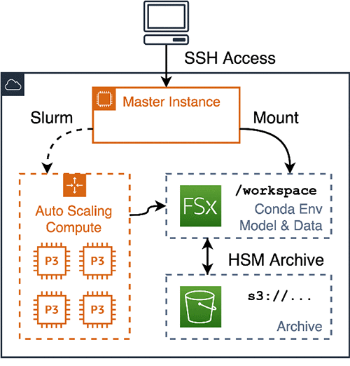
AWS ParallelCluster enables a scalable research workflow built around on-demand allocation of compute resources. Rather than working with, and potentially underutilizing, a single high-power GPU-enabled workstation, AWS ParallelCluster manages an on-demand fleet of GPU-enabled compute workers. This allows trivial scale-up for parallel training experiments and automatic scale-down when resources aren’t required, minimizing cost and (most importantly) saving researcher time. An attached Amazon FSx file system takes advantage of a traditional high-performance Lustre file system during development, but archives models and data into the low-cost Amazon S3.

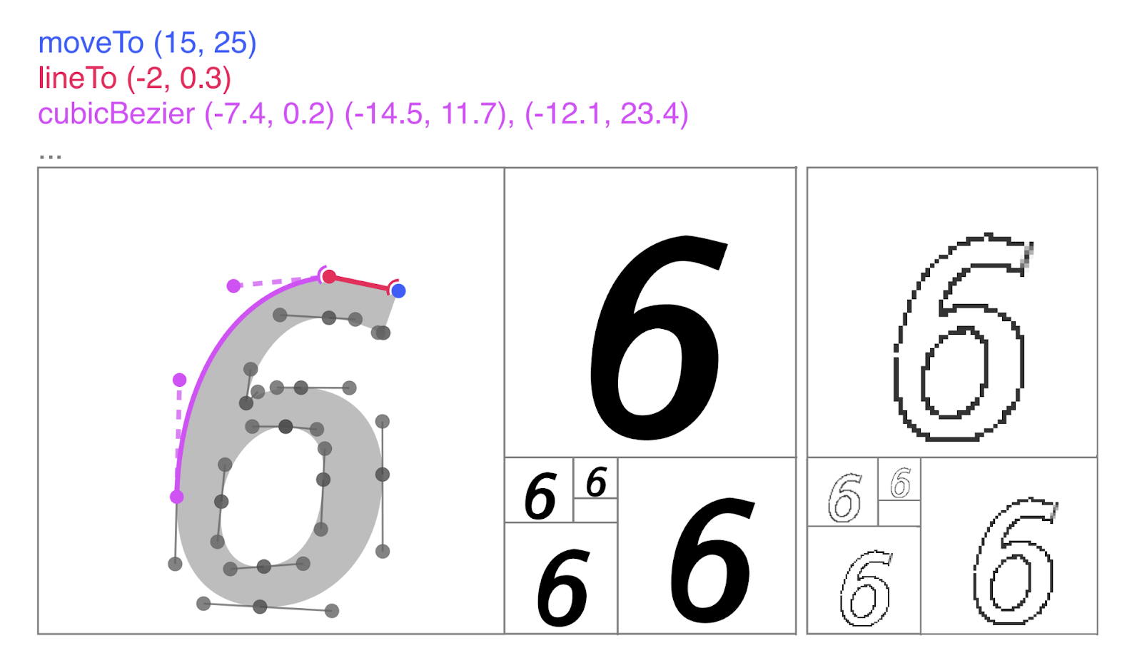
The following graphic shows an AWS ParallelCluster-based research environment. Autoscaled Amazon EC2 resources access remote storage, with models and data archived to S3.

This post shows you how to set up, run, and tear down a complete AWS ParallelCluster environment implementing this architecture. The post runs two NLP tutorials, fine-tuning a BERT model on a paraphrasing task and training an English-German machine translation model. This includes the following steps:

  1. AWS ParallelCluster configuration and setup
  2. Conda-based installation of your ML and NLP packages
  3. Initial interactive model training
  4. Parallel model training and evaluation
  5. Data archiving and cluster teardown

The tutorial lays out a workflow using standard tools, and you can adapt it to your research requirements.

Prerequisites

This post uses a combination of m5 and p3 EC2 instances and Amazon FSx and Amazon S3 storage. Furthermore, because you are using GPU-enabled instances for training, this tutorial takes your account out of the free AWS tier. Before you begin, complete the following prerequisites:

  1. Set up an AWS account and create an access token with administrator permissions.
  2. Request quota increases in your target AWS Region for at least one m5.xlarge, three p3.2xlarge, and three p3.8xlarge On-Demand Instances.

Setting up your client and cluster

Start with a one-time setup and configuration of your workstation with the aws-parallelcluster client in a dedicated Conda environment. You reuse this pattern again later when setting up isolated environments for each subproject that contains a precise set of dependencies required to reproduce your work.

Installing Conda

Perform a one-time installation of a base Miniconda environment and initialize your shell to enable Conda. This post works from a macOS workstation; use the download URL for your preferred platform. This configuration sets up a base environment and activates it in your interactive shell. See the following code:

@work:~$ wget -O miniconda.sh 
    "https://repo.anaconda.com/miniconda/Miniconda3-latest-MacOSX-x86_64.sh" 
    && bash miniconda.sh -p ~/.conda 
    && ~/.conda/bin/conda init

Setting up your client environment

Install AWS ParallelCluster and the AWS CLI tools using a Conda environment called pcluster_client. This environment provides separation between the client and your system environment. First, write an environment.yml file specifying the environment name and dependency versions. Call conda env update to download and install the libraries. See the following code:

(base) @work:~$ cat > pcluster_client.environment.yml <<EOF
name: pcluster_client
dependencies:
  - python=3.7
  - pip
  - conda-forge::jq
  - conda-forge::awscli
  - pip:
    - aws-parallelcluster >= 2.4
EOF

(base) @work:~$ conda env update -f pcluster_client.environment.yml

Configuring pcluster and creating storage

To configure AWS ParallelCluster, conda activate your pcluster_client environment and configure aws and pcluster via the default configuration flow. For more information, see Configuring AWS ParallelCluster.

During configuration, upload your id_rsa public key to AWS and store your private key locally, which you use to access your pcluster instances. See the following code:

(base) @work:~$ conda activate pcluster_client
(pcluster_client) @work:~$ aws configure
  [...]
(pcluster_client) @work:~$ aws ec2 import-key-pair 
    --key-name $USER --public-key-material file://~/.ssh/id_rsa.pub
{
    "KeyFingerprint": [...]
    [...]
}
(pcluster_client) @work:~$ pcluster configure
  [...]

After configuring AWS ParallelCluster, create an S3 bucket for persistent storage of your data and models with the following code:

(pcluster_client) @work:~$ export AWS_ACCOUNT=$(aws sts get-caller-identity | jq -r ".Account")
(pcluster_client) @work:~$ export S3_BUCKET=pcluster-training-workspace-$AWS_ACCOUNT
(pcluster_client) @work:~$ aws s3 mb s3://$S3_BUCKET
  make_bucket: pcluster-training-workspace-[...account id...]

Add config entries for a GPU-enabled cluster and Amazon FSx file system with the following code:

(pcluster_client) @work:~$ cat >> ~/.parallelcluster/config <<EOF

[cluster p3.2xlarge]
key_name                 = $USER
vpc_settings             = public

scheduler                = slurm
base_os                  = centos7
fsx_settings             = workspace

initial_queue_size       = 1
max_queue_size           = 3

master_instance_type     = m5.xlarge
compute_instance_type    = p3.2xlarge

[fsx workspace]
shared_dir = /workspace
storage_capacity = 3600
import_path = s3://$S3_BUCKET
export_path = s3://$S3_BUCKET
imported_file_chunk_size = 1024

EOF

Creating and bootstrapping your cluster

After configuration, bring your cluster online. This command creates a persistent master instance, attaches an Amazon FSx file system, and sets up a p3 class Auto Scaling group. After cluster creation is complete, set up Miniconda again, this time installing it onto the /workspace file system accessible on all master and compute nodes. See the following code:

(pcluster_client) @work:~$ pcluster create -t p3.2xlarge training
Beginning cluster creation for cluster: training
Creating stack named: parallelcluster-training
Status: [...]

(pcluster_client) @work:~$ pcluster ssh training

[centos@ip-172-31-48-17 ~]$ wget -O miniconda.sh 
    "https://repo.anaconda.com/miniconda/Miniconda3-latest-Linux-x86_64.sh" 
    && bash miniconda.sh -p /workspace/.conda 
    && /workspace/.conda/bin/conda init
[centos@ip-172-31-48-17 ~]$ exit

Your compute cluster now contains a single m5 class instance, with p3.2xlarge instances available via the slurm job manager. You can use an interactive salloc session to access your p3 resources via srun commands. An important implication of your autoscaled cluster strategy is that while all code and data are available across the cluster, access to attached GPUs is limited to compute nodes accessed via srun. You can demonstrate this via calls to nvidia-smi, which reports the status of attached resources. See the following code:

(pcluster_client) @work:~$ pcluster ssh training

# Execution on the master node can not access gpu resources.
(base) [centos@ip-172-31-48-17 ~]$ hostname
ip-172-31-48-17
(base) [centos@ip-172-31-48-17 ~]$ nvidia-smi
NVIDIA-SMI has failed [...]

# Use salloc to bring a compute node online, then use calls to srun to
# execute commands on the GPU-enabled compute node.
(base) [centos@ip-172-31-48-17 ~]$ salloc
salloc: Required node not available (down, drained or reserved)
salloc: Pending job allocation 2
salloc: job 2 queued and waiting for resources
salloc: job 2 has been allocated resources
salloc: Granted job allocation 2

(base) [centos@ip-172-31-48-17 ~]$ srun hostname
ip-172-31-48-226

(base) [centos@ip-172-31-48-17 ~]$ srun nvidia-smi
+-----------------------------------------------------------------------------+
| NVIDIA-SMI 418.56       Driver Version: 418.56       CUDA Version: 10.1     |
|-------------------------------+----------------------+----------------------+
| GPU  Name        Persistence-M| Bus-Id        Disp.A | Volatile Uncorr. ECC |
| Fan  Temp  Perf  Pwr:Usage/Cap|         Memory-Usage | GPU-Util  Compute M. |
|===============================+======================+======================|
|   0  Tesla V100-SXM2...  Off  | 00000000:00:1E.0 Off |                    0 |
| N/A   34C    P0    39W / 300W |      0MiB / 16130MiB |      0%      Default |
+-------------------------------+----------------------+----------------------+

+-----------------------------------------------------------------------------+
| Processes:                                                       GPU Memory |
|  GPU       PID   Type   Process name                             Usage      |
|=============================================================================|
|  No running processes found                                                 |
+-----------------------------------------------------------------------------+
(base) [centos@ip-172-31-48-17 ~]$ exit
exit
salloc: Relinquishing job allocation 2

AWS ParallelCluster performs automatic management of your compute Auto Scaling group. This keeps a compute node running and available for the lifetime of your salloc and terminates the idle compute node several minutes after the job ends.

Model training

Initial GPU-enabled interactive training

For an initial research task, run a standard natural language process workflow, fine-tuning a pre-trained BERT model onto a specific subtask. Establish a working environment with your model dependencies, download the pre-trained model and training data, and run fine-tuning training on a GPU. For more information about PyTorch pre-trained BERT examples, see the GitHub repo.

First, run a one-time setup of your project: a Conda environment with library dependencies and a workspace with training data. Write an environment.yml specifying the dependencies for your project, call conda env update to create and install the environment, and call conda env activate. Fetch your training data into /workspace/bert_tuning. See the following code:

(base) [centos@ip-172-31-48-17 ]$ mkdir /workspace/bert_tuning
 (base) [centos@ip-172-31-48-17 ]$ cd /workspace/bert_tuning

(base) [centos@ip-172-31-48-17 bert_tuning]$ cat > environment.yml <<EOF
name: bert_tuning
dependencies:
  - python=3.7
  - pytorch::pytorch=1.1
  - scipy=1.2
  - scikit-learn=0.21
  - pip
  - requests
  - tqdm
  - boto3
  - pip:
    - pytorch_pretrained_bert==0.6.2
EOF

(base) [centos@ip-172-31-48-17 bert_tuning]$ conda env update
[...]
# To activate this environment, use
#
#     $ conda activate bert_tuning

(base) [centos@ip-172-31-48-17 bert_tuning]$ conda activate bert_tuning

(bert_tuning) [centos@ip-172-31-48-17 bert_tuning]$ wget 
   https://gist.githubusercontent.com/W4ngatang/60c2bdb54d156a41194446737ce03e2e/raw/17b8dd0d724281ed7c3b2aeeda662b92809aadd5/download_glue_data.py
(bert_tuning) [centos@ip-172-31-48-17 bert_tuning]$ python download_glue_data.py --data_dir glue
Downloading and extracting Cola...
[...]
        Completed!

After downloading your dependencies, fetch the training script and run fine-tuning in an interactive session. The only difference from the documented non-cluster example is that you run your training via salloc --exclusive srun rather than directly invoking the training script. The /workspace Amazon FSx file system allows the compute node to access your Conda environment’s installed libraries and your model definition, training data, and model checkpoints. As before, allocate a GPU-enabled node for the training run, which terminates after your run is complete. See the following code:

(bert_tuning) [centos@ip-172-31-48-17 bert_tuning]$ wget 
  https://raw.githubusercontent.com/huggingface/pytorch-pretrained-BERT/v0.6.2/examples/run_classifier.py
(bert_tuning) [centos@ip-172-31-48-17 bert_tuning]$ salloc --exclusive srun 
python run_classifier.py 
  --task_name MRPC 
  --do_train 
  --do_eval 
  --do_lower_case 
  --data_dir glue/MRPC/ 
  --bert_model bert-base-uncased 
  --max_seq_length 128 
  --train_batch_size 32 
  --learning_rate 2e-5 
  --num_train_epochs 3.0 
  --output_dir mrpc_output
salloc: Required node not available (down, drained or reserved)
salloc: Pending job allocation 3
salloc: job 3 queued and waiting for resources
salloc: job 3 has been allocated resources
salloc: Granted job allocation 3
06/12/2019 02:15:36 - INFO - __main__ -   device: cuda n_gpu: 1, distributed training: False, 16-bits training: False
[...]
Epoch:  100%|██████████| 3/3 [01:11<00:35, 35.90s/it] 
[...]
Evaluating: 100%|██████████| 51/51 [00:01<00:00, 41.42it/s]
06/12/2019 02:17:48 - INFO - __main__ -   ***** Eval results *****
06/12/2019 02:17:48 - INFO - __main__ -     acc = 0.8455882352941176
06/12/2019 02:17:48 - INFO - __main__ -     acc_and_f1 = 0.867627742865973
06/12/2019 02:17:48 - INFO - __main__ -     eval_loss = 0.42869279022310297
06/12/2019 02:17:48 - INFO - __main__ -     f1 = 0.8896672504378283
06/12/2019 02:17:48 - INFO - __main__ -     global_step = 345
06/12/2019 02:17:48 - INFO - __main__ -     loss = 0.15244172460035138
salloc: Relinquishing job allocation 3

(bert_tuning) [centos@ip-172-31-48-17 bert_tuning]$ exit

Multi-GPU training

Using salloc is useful for interactive model development, short training jobs, and testing. However, the majority of modern research requires multiple long-running training jobs for model development and tuning. To support more compute-intensive experimentation, update your cluster to multi-GPU compute instances and use sbatch for non-interactive training. Enqueue multiple training jobs for an experiment and let AWS ParallelCluster scale up your compute group for the run and scale down after the experiment is complete.

From your workstation, add configuration for a multi-GPU cluster, shut down any remaining single-GPU nodes, and update your cluster configuration to multi-GPU p3.8xlarge compute instances. See the following code:

(pcluster_client) @work:~$ cat >> ~/.parallelcluster/config <<EOF

[cluster p3.8xlarge]
key_name                 = $USER
vpc_settings             = public

scheduler                = slurm
base_os                  = centos7
fsx_settings             = workspace

initial_queue_size       = 1
max_queue_size           = 3

master_instance_type     = m5.xlarge
compute_instance_type    = p3.8xlarge

EOF

(pcluster_client) @work:~$ (
       pcluster stop training
       pcluster update training -t p3.8xlarge
       pcluster start training 
   )

Stopping compute fleet : training
Updating: training
Calling update_stack
Status: parallelcluster-training - UPDATE_COMPLETE
Starting compute fleet : training

(pcluster_client) @work:~$ pcluster ssh training

(base) [centos@ip-172-31-48-17 ~]$ salloc srun nvidia-smi
salloc: Granted job allocation 4
Wed Jun 12 06:02:25 2019
+-----------------------------------------------------------------------------+
| NVIDIA-SMI 418.56       Driver Version: 418.56       CUDA Version: 10.1     |
|-------------------------------+----------------------+----------------------+
| GPU  Name        Persistence-M| Bus-Id        Disp.A | Volatile Uncorr. ECC |
| Fan  Temp  Perf  Pwr:Usage/Cap|         Memory-Usage | GPU-Util  Compute M. |
|===============================+======================+======================|
|   0  Tesla V100-SXM2...  Off  | 00000000:00:1B.0 Off |                    0 |
| N/A   47C    P0    52W / 300W |      0MiB / 16130MiB |      0%      Default |
+-------------------------------+----------------------+----------------------+
|   1  Tesla V100-SXM2...  Off  | 00000000:00:1C.0 Off |                    0 |
| N/A   46C    P0    52W / 300W |      0MiB / 16130MiB |      0%      Default |
+-------------------------------+----------------------+----------------------+
|   2  Tesla V100-SXM2...  Off  | 00000000:00:1D.0 Off |                    0 |
| N/A   49C    P0    58W / 300W |      0MiB / 16130MiB |      0%      Default |
+-------------------------------+----------------------+----------------------+
|   3  Tesla V100-SXM2...  Off  | 00000000:00:1E.0 Off |                    0 |
| N/A   47C    P0    57W / 300W |      0MiB / 16130MiB |      0%      Default |
+-------------------------------+----------------------+----------------------+

+-----------------------------------------------------------------------------+
| Processes:                                                       GPU Memory |
|  GPU       PID   Type   Process name                             Usage      |
|=============================================================================|
|  No running processes found                                                 |
+-----------------------------------------------------------------------------+
salloc: Relinquishing job allocation 4

This post retrains a transformer-based English-to-German translation model using the FairSeq NLP framework. As before, set up a new workspace and environment and download training data. See the following code:

(base) [centos@ip-172-31-48-17 ~]$ mkdir /workspace/translation
(base) [centos@ip-172-31-48-17 ~]$ cd /workspace/translation

(base) [centos@ip-172-31-48-17 translation]$ cat > environment.yml <<EOF
name: translation
dependencies:
  - python=3.7
  - pytorch::pytorch=1.1
  - pip
  - tqdm
  - pip:
    - fairseq==0.6.2
EOF

(translation) [centos@ip-172-31-48-17 translation]$ conda env update && conda activate translation

(translation) [centos@ip-172-31-48-17 translation]$ wget 
  https://raw.githubusercontent.com/pytorch/fairseq/v0.6.2/examples/translation/prepare-iwslt14.sh 
  && bash prepare-iwslt14.sh

[...]

(translation) [centos@ip-172-31-48-17 translation]$ fairseq-preprocess 
  --source-lang de --target-lang en 
  --trainpref iwslt14.tokenized.de-en/train 
  --validpref iwslt14.tokenized.de-en/valid 
  --testpref  iwslt14.tokenized.de-en/test 
  --destdir data-bin/iwslt14.tokenized.de-en
    
[...]
| Wrote preprocessed data to data-bin/iwslt14.tokenized.de-en

After downloading and preprocessing your training data, write your training script and launch a quick interactive training run to confirm that your script launches and successfully trains for several epochs. Your first job is limited to a single GPU via CUDA_VISIBLE_DEVICES and should train in approximately 60 seconds/epoch; after an epoch or so, interrupt with ctrl-C. Because your underlying model supports distributed data-parallel training, you can expect nearly linear performance scaling with additional GPUs on a single worker. Training in a second job with all four devices should train in approximately 15–20 seconds/epoch, confirming effective multi-GPU scaling, which you again interrupt. See the following code:

(translation) [centos@ip-172-31-48-17 translation]$ mkdir -p checkpoints/transformer
(translation) [centos@ip-172-31-48-17 translation]$ (cat > train_transformer && chmod +x train_transformer) <<EOF
#!/bin/bash
fairseq-train data-bin/iwslt14.tokenized.de-en 
  -a transformer_iwslt_de_en --optimizer adam --lr 0.0005 -s de -t en 
  --label-smoothing 0.1 --dropout 0.3 --max-tokens 4000 
  --min-lr '1e-09' --lr-scheduler inverse_sqrt --weight-decay 0.0001 
  --criterion label_smoothed_cross_entropy --max-update 50000 
  --warmup-updates 4000 --warmup-init-lr '1e-07' 
  --adam-betas '(0.9, 0.98)' --fp16 
  --save-dir checkpoints/transformer
EOF

(translation) [centos@ip-172-31-48-17 translation]$ CUDA_VISIBLE_DEVICES=0 salloc --exclusive 
  srun -X --pty ./train_transformer
  
  [...]
| training on 1 GPUs
  [...]
  ^C
  [...]
  KeyboardInterrupt
  
(translation) [centos@ip-172-31-48-17 translation]$ salloc --exclusive 
  srun -X --pty ./train_transformer
  
  [...]
| training on 4 GPUs
  [...]
  ^C
  [...]
  KeyboardInterrupt

After your initial validation, run sbatch to schedule your full training run. The sinfo command provides information about your running cluster, and squeue shows the status of your batch job. tail on the job log allows you to monitor training progress, and ssh access to the compute node address reported by squeue allows you to check resource utilization. As before, AWS ParallelCluster scales up your compute cluster for the batch training job and releases the GPU-enabled instances after batch training is complete. See the following code:

(translation) [centos@ip-172-31-48-17 translation]$ sbatch --exclusive 
  --output=train_transformer.log 
  ./train_transformer

Submitted batch job 9.

(translation) [centos@ip-172-31-21-188 translation]$ sinfo
PARTITION AVAIL  TIMELIMIT  NODES  STATE NODELIST
compute*     up   infinite      1  alloc ip-172-31-20-225

(translation) [centos@ip-172-31-21-188 translation]$ squeue
             JOBID PARTITION     NAME     USER ST       TIME  NODES NODELIST(REASON)
                 9   compute   sbatch   centos  R       0:22      1 ip-172-31-20-225
                
(translation) [centos@ip-172-31-21-188 translation]$ tail train_transformer.log
[...]
| loaded checkpoint checkpoints/transformer/checkpoint_last.pt (epoch 5 @ 1413 updates)
| epoch 006 | loss 7.268 | [...]
| epoch 006 | valid on 'valid' subset | loss 6.806 | [...]

(translation) [centos@ip-172-31-21-188 translation]$ ssh -t ip-172-31-20-225 watch nvidia-smi

+-----------------------------------------------------------------------------+
| NVIDIA-SMI 418.56       Driver Version: 418.56       CUDA Version: 10.1     |
|-------------------------------+----------------------+----------------------+
| GPU  Name        Persistence-M| Bus-Id        Disp.A | Volatile Uncorr. ECC |
| Fan  Temp  Perf  Pwr:Usage/Cap|         Memory-Usage | GPU-Util  Compute M. |
|===============================+======================+======================|
|   0  Tesla V100-SXM2...  Off  | 00000000:00:1B.0 Off |                    0 |
| N/A   63C    P0   214W / 300W |   3900MiB / 16130MiB |     83%      Default |
+-------------------------------+----------------------+----------------------+
|   1  Tesla V100-SXM2...  Off  | 00000000:00:1C.0 Off |                    0 |
| N/A   64C    P0   175W / 300W |   4110MiB / 16130MiB |     82%      Default |
+-------------------------------+----------------------+----------------------+
|   2  Tesla V100-SXM2...  Off  | 00000000:00:1D.0 Off |                    0 |
| N/A   60C    P0   164W / 300W |   4026MiB / 16130MiB |     65%      Default |
+-------------------------------+----------------------+----------------------+
|   3  Tesla V100-SXM2...  Off  | 00000000:00:1E.0 Off |                    0 |
| N/A   62C    P0   115W / 300W |   3994MiB / 16130MiB |     74%      Default |
+-------------------------------+----------------------+----------------------+

+-----------------------------------------------------------------------------+
| Processes:                                                       GPU Memory |
|  GPU       PID   Type   Process name                             Usage      |
|=============================================================================|
|    0     41837      C   ...ntos/.conda/envs/translation/bin/python  3889MiB |
|    1     41838      C   ...ntos/.conda/envs/translation/bin/python  4099MiB |
|    2     41839      C   ...ntos/.conda/envs/translation/bin/python  4015MiB |
|    3     41840      C   ...ntos/.conda/envs/translation/bin/python  3983MiB |
+-----------------------------------------------------------------------------+

The job takes approximately 80–90 minutes to complete. You can now evaluate your model via interactive translation. See the following code:

(translation) [centos@ip-172-31-21-188 translation]$ squeue
             JOBID PARTITION     NAME     USER ST       TIME  NODES NODELIST(REASON)
(translation) [centos@ip-172-31-21-188 translation]$ fairseq-interactive 
  data-bin/iwslt14.tokenized.de-en 
  --path checkpoints/transformer/checkpoint_best.pt --beam 5 --remove-bpe <<EOF
hallo welt
EOF

Namespace([...])
| [de] dictionary: 8848 types
| [en] dictionary: 6632 types
| loading model(s) from checkpoints/transformer/checkpoint_best.pt
| Type the input sentence and press return:
S-0    hallo welt
H-0    -0.32129842042922974    hello world .
P-0    -0.8112 -0.0095 -0.4157 -0.2850 -0.0851

Jupyter and other HTTP services

Interactive notebook-based development is frequently used for data exploration, model analysis, and prototyping. You can launch and access a notebook server running on your AWS ParallelCluster workers. Add jupyterlab to the project’s workspace environment and srun the notebook. See the following code:

(translation) [centos@ip-172-31-48-17 translation]$ conda install jupyterlab

[...]

# unset XDG_RUNTIME_DIR and listen on node name to allow ssh tunnel.
(translation) [centos@ip-172-31-48-17 translation]$ 
  XDG_RUNTIME_DIR= 
  salloc --exclusive srun -X --pty bash -c 
  'jupyter lab --ip=$SLURMD_NODENAME'

[...]
The Jupyter Notebook is running at:
http://ip-172-31-21-236:8888/?token=[...token...]

In a separate terminal, set up a pcluster ssh tunnel to the notebook worker using the node address and access token reported by Jupyter and open a local browser. See the following code:

(pcluster_client) @work:~$ pcluster ssh training -L 8888:ip-172-31-21-236:8888 -N&
(pcluster_client) @work:~$ jobs
[1]+  Running.  pcluster ssh training -L 8888:ip-172-31-21-236:8888 -N &

(pcluster_client) @work:~$ open http://localhost:8888/?token=[...token...]

You can use a similar approach to run tools such as tensorboard in your cluster environment.

Storage and cluster teardown

After completing model training and evaluation, you can archive your /workspace file system to Amazon S3 via Amazon FSx’s hierarchical storage support. For more information, see Using Data Repositories. After the hsm_archive actions complete in approximately 60–90 minutes, verify the contents of your s3 export bucket via the AWS CLI with the following code:

(pcluster_client) @work:~$ pcluster ssh training

# Find and archive all files in the /workspace
(base) [centos@ip-172-31-48-17 translation]$ 
  find /workspace -type f -print0 
  | xargs -0 -n 16 sudo lfs hsm_archive
  
# Returns 0 when all archive operations are complete
(base) [centos@ip-172-31-48-17 translation]$ 
  find /workspace -type f -print0 
  | xargs -0 -n 16 -P 8 sudo lfs hsm_action | grep "ARCHIVE" | wc -l
  
0

(base) [centos@ip-172-31-48-17 translation]$ exit

(pcluster_client) @work:~$ aws s3 ls 
    s3://pcluster-training-workspace-$(aws sts get-caller-identity | jq -r ".Account")
                           
    PRE bert_tuning/
    PRE translation/
    
(pcluster_client) @work:~$ pcluster delete training
Deleting: training
[...]

A later call to pcluster create with the same configuration restores your cluster, pre-populating /workspace from your S3 archive.

Multiple clusters

You can use AWS ParallelCluster to manage multiple concurrent compute clusters. For instance, you can use a mix of CPU and GPU clusters to support preprocessing or analysis tasks that involve significant CPU-bound processing. Additionally, this can provide independent clusters for multiple researchers in a single shared AWS workspace.

Adapting this workflow to a multi-cluster configuration is relatively simple. Set up a standalone Amazon FSx file system and manage its lifecycle via existing CloudFormation templates in the amazon-fsx-workshop/lustre GitHub repo. Specify an export prefix and update ~/.parallelcluster/config with the following code:

[fsx workspace]
       shared_dir = /workspace
       fsx_fs_id = <filesystem id>

Multiple clusters now share a /workspace file system, decoupled from the lifetime of any individual cluster. You can use calls to lfs hsm_archive from any cluster to back up file system contents to S3, potentially via a nightly cron.

Capacity management

AWS ParallelCluster manages a compute cluster of EC2 instances via a standard Auto Scaling group, allowing you to use existing AWS-native tools for capacity management as you scale clusters. AWS ParallelCluster has built-in support for using Spot Instances within compute fleets via cluster_type configuration, and uses Reserved Instance capacity if available. You can use On-Demand Capacity Reservations so AWS ParallelCluster can rapidly scale to match your target compute fleet size.

Conclusion

If you wish to maintain more direct control over your computing infrastructure, an AWS ParallelCluster-based workflow provides an ideal working environment for applied machine learning research. Rapid cluster setup, scaling, and updates allow interactive exploration of a modeling task, including identification of a proper instance type and multi-instance scaling for parallel training runs. Conda environments and a high-performance Amazon FSx file system provide a familiar file interface and handle the critical, but undifferentiated, heavy lifting of reproducibly archiving model artifacts to S3 transparently.

For more information about configuring AWS ParallelCluster and building an interactive and scalable ML or HPC research environment, see the AWS ParallelCluster User Guide or the aws-parallelcluster GitHub repo.


About the author

Alex Ford is an Applied Scientist with AWS. He is passionate about emerging applications at the intersection of machine learning and the natural sciences. In his spare time, he explores the geography and geology of the Cascadia subduction zone, with deep affection for the Index batholith.

The Visual Task Adaptation Benchmark

Deep learning has revolutionized computer vision, with state-of-the-art deep networks learning useful representations directly from raw pixels, leading to unprecedented performance on many vision tasks. However, learning these representations from scratch typically requires hundreds of thousands of training examples. This burden can be reduced by using pre-trained representations, which have become widely available through services such as TensorFlow Hub (TF Hub) and PyTorch Hub. But their ubiquity can itself be a hindrance. For example, for the task of extracting features from images, there can be over 100 models from which to choose. It is hard to know which methods provide the best representations, since different sub-fields use different evaluation protocols, which do not always reflect the final performance on new tasks.

The overarching goal of representation research is to learn representations a single time on large amounts of generic data without the need to train them from scratch for each task, thus reducing data requirements across all vision tasks. But in order to reach that goal, the research community must have a uniform benchmark against which existing and future methods can be evaluated.

To address this problem, we are releasing “The Visual Task Adaptation Benchmark” (VTAB, available on GitHub), a diverse, realistic, and challenging representation benchmark based on one principle — a better representation is one that yields better performance on unseen tasks, with limited in-domain data. Inspired by benchmarks that have driven progress in other fields of machine learning (ML), such as ImageNet for natural image classification, GLUE for Natural Language Processing, and Atari for reinforcement learning, VTAB follows similar guidelines: (i) minimal constraints on solutions to encourage creativity; (ii) a focus on practical considerations; and (iii) challenging tasks for evaluation.

The Benchmark
VTAB is an evaluation protocol designed to measure progress towards general and useful visual representations, and consists of a suite of evaluation vision tasks that a learning algorithm must solve. These algorithms may use pre-trained visual representations to assist them and must satisfy only two requirements:

    i) They must not be pre-trained on any of the data (labels or input images) used in the downstream evaluation tasks.
    ii) They must not contain hardcoded, task-specific, logic. Alternatively put, the evaluation tasks must be treated like a test set — unseen.

These constraints ensure that solutions that are successful when applied to VTAB will be able to generalize to future tasks.

The VTAB protocol begins with the application of an algorithm (A) to a number of independent tasks, drawn from a broad distribution of vision problems. The algorithm may be pre-trained on upstream data to yield a model that contains visual representations, but it must also define an adaptation strategy that consumes a small training set for each downstream task and return a model that makes task-specific predictions. The algorithm’s final score is its average test score across tasks.

The VTAB protocol. Algorithm A is applied to many tasks T, drawn from a broad distribution of vision problems PT. In the example, pet classification, remote sensing, and maze localization are shown.

VTAB includes 19 evaluation tasks that span a variety of domains, divided into three groups — natural, specialized, and structured. Natural image tasks include images of the natural world captured through standard cameras, representing generic objects, fine-grained classes, or abstract concepts. Specialized tasks utilize images captured using specialist equipment, such as medical images or remote sensing. The structured tasks often derive from artificial environments that target understanding of specific changes between images, such as predicting the distance to an object in a 3D scene (e.g., DeepMind Lab), counting objects (e.g., CLEVR), or detecting orientation (e.g., dSprites for disentangled representations).

While highly diverse, all of the tasks in VTAB share one common feature — people can solve them relatively easily after training on just a few examples. To assess algorithmic generalization to new tasks with limited data, performance is evaluated using only 1000 examples per task. Evaluation using the full dataset can be performed for comparison with previous publications.

Findings Using VTAB
We performed a large scale study testing a number of popular visual representation learning algorithms against VTAB. The study included generative models (GANs and VAEs), self-supervised models, semi-supervised models and supervised models. All of the algorithms were pre-trained on the ImageNet dataset. We also compared each of these approaches using no pre-trained representations, i.e., training “from-scratch”. The figure below summarizes the main pattern of results.

Performance of different classes of representation learning algorithms across different task groups: natural, specialized and structured. Each bar shows the average performance of all methods in that class across all tasks in the group.

Overall we find that generative models do not perform as well as the other methods, even worse than from-scratch training. However, self-supervised models perform much better, significantly outperforming from-scratch training. Better still is supervised learning using the ImageNet labels. Interestingly, while supervised learning is significantly better on the Natural group of tasks, self-supervised learning is close on the other two groups whose domains are more dissimilar to ImageNet.

The best performing representation learning algorithm, of those we tested, is S4L, which combines both supervised and self-supervised pre-training losses. The figure below contrasts S4L with standard supervised ImageNet pre-training. S4L appears to improve performance particularly on the Structured tasks. However, representation learning yields a much smaller benefit over training from-scratch groups other than the Natural tasks, indicating that there is much progress required to attain a universal visual representation.

Top: Performance of S4L versus from-scratch training. Each bar corresponds to a task. Positive-valued bars indicate tasks where S4L outperforms from-scratch. Negative bars indicate that from-scratch performed better. Bottom: S4L versus Supervised training on ImageNet. Positive bars indicate that S4L performs better. The bar colour indicates the task group: Red=Natural, Green=Specialized, Blue=Structured. We can see that additional self-supervision tends to help on structured tasks beyond just using ImageNet labels.

Summary
The code to run VTAB is available on GitHub, including the 19 evaluation datasets and exact data splits. Having a publicly available set of benchmarks ensures the reproducibility of results. Progress is tracked with the public leaderboard, and the models evaluated are uploaded to TF Hub for public use and reproduction. A shell script is provided to perform adaptation and evaluation on all the tasks, with a standardized evaluation protocol making VTAB readily accessible across the industry. Since VTAB can be executed on both TPU and GPU, it is highly efficient. One can obtain comparable results with a single NVIDIA Tesla P100 accelerator in a few hours.

The Visual Task Adaptation Benchmark has helped us better understand which visual representations generalize to the broad spectrum of vision tasks, and provides direction for future research. We hope these resources are useful in driving progress toward general and practical visual representations, and as a result, affords deep learning to the long tail of vision problems with limited labelled data.

Acknowledgements
The core team behind this work includes Joan Puigcerver, Alexander Kolesnikov, Pierre Ruyssen, Carlos Riquelme, Mario Lucic, Josip Djolonga, Andre Susano Pinto, Maxim Neumann, Alexey Dosovitskiy, Lucas Beyer, Olivier Bachem, Michael Tschannen, Marcin Michalski, Olivier Bousquet, and Sylvain Gelly.

NVIDIA Shows Its Prowess in First AI Inference Benchmarks

Those who are keeping score in AI know that NVIDIA GPUs set the performance standards for training neural networks in data centers in December and again in July. Industry benchmarks released today show we’re setting the pace for running those AI networks in and outside data centers, too.

NVIDIA Turing GPUs and our Xavier system-on-a-chip posted leadership results in MLPerf Inference 0.5, the first independent benchmarks for AI inference. Before today, the industry was hungry for objective metrics on inference because its expected to be the largest and most competitive slice of the AI market.

Among a dozen participating companies, only the NVIDIA AI platform had results across all five inference tests created by MLPerf, an industry benchmarking group formed in May 2018. That’s a testament to the maturity of our CUDA-X AI and TensorRT software. They ease the job of harnessing all our GPUs that span uses from data center to the edge.

MLPerf defined five inference benchmarks that cover three established AI applications — image classification, object detection and translation. Each benchmark has four aspects. Server and offline scenarios are most relevant for data center uses cases, while single- and multi-stream scenarios speak to the needs of edge devices and SoCs.

Chart showing MLPerf use cases and scenarios

NVIDIA topped all five benchmarks for both data center scenarios (offline and server), with Turing GPUs providing the highest performance per processor among commercially available products.

MLPerf chart showing NVIDIA Turing performance
NVIDIA Turing topped among the commercially available processors in MLPerf scenarios geared for the data center.1

The offline scenario represents data center tasks such as tagging photos, where all the data is available locally. The server scenario reflects jobs such as online translation services, where data and requests are arriving randomly in bursts and lulls.

For its part, Xavier ranked as the highest performer under both edge-focused scenarios (single- and multi-stream) among commercially available edge and mobile SoCs.

An industrial inspection camera identifying defects in a fast-moving production line is a good example of a single-stream task. The multi-stream scenario tests how many feeds a chip can handle — a key capability for self-driving cars that might use a half-dozen cameras or more.

MPLerf chart showing NVIDIA Xavier performance
NVIDIA’s Xavier topped the group of commercially available edge and mobile SoCs in MLPerf scenarios geared for the edge.2

The results reveal the power of our CUDA and TensorRT software. They provide a common platform that enables us to show leadership results across multiple products and use cases, a capability unique to NVIDIA.

We competed in data center scenarios with two GPUs. Our TITAN RTX demonstrated the full potential of our Turing-class GPUs, especially in demanding tasks such as running a GNMT model used for language translation.

The versatile and widely used NVIDIA T4 Tensor Core GPU showed strong results across several scenarios. These 70-watt GPUs are designed to easily fit into any server with PCIe slots, enabling users to expand their computing power as needed for inference jobs known to scale well.

MLPerf has broad backing from industry and academia. Its members include Arm, Facebook, Futurewei, General Motors, Google, Harvard University, Intel, MediaTek, Microsoft, NVIDIA and Xilinx. To its credit, the new benchmarks attracted significantly more participants than two prior training competitions.

NVIDIA demonstrated its support for the work by submitting results in 19 of 20 scenarios, using three products in a total of four configurations. Our partner Dell EMC and our customer Alibaba also submitted results using NVIDIA GPUs. Together, we gave users a broader picture of the potential of our product portfolio than any other participant.

Fresh Perspectives, New Products

Inference is the process of running AI models in real-time production systems to filter actionable insights from a haystack of data. It’s an emerging technology that’s still evolving, and NVIDIA isn’t standing still.

Today we announced a low-power version of the Xavier SoC used in the MLPerf tests. At full throttle, Jetson Xavier NX delivers up to 21 TOPS while consuming just 15 watts. It aims to drive a new generation of performance-hungry, power-pinching robots, drones and other autonomous devices.

In addition to the new hardware, NVIDIA released new TensorRT 6 optimizations used in the MLPerf benchmarks as open source on GitHub. You can learn more about the optimizations in this MLPerf developer blog. We continuously evolve this software so our users can reap benefits from increasing AI automation and performance.

Making Inference Easier for Many

One big takeaway from today’s MLPerf tests is inference is hard. For instance, in actual workloads inference is even more demanding than in the benchmarks because it requires significant pre- and post-processing steps.

In his keynote address at GTC last year, NVIDIA founder and CEO Jensen Huang compressed the complexities into one word: PLASTER. Modern AI inference requires excellence in Programmability, Latency, Accuracy, Size-of-model, Throughput, Energy efficiency and Rate of Learning, he said.

That’s why users are increasingly embracing high-performance NVIDIA GPUs and software to handle demanding inference jobs. They include a who’s who of forward-thinking companies such as BMW, Capital One, Cisco, Expedia, John Deere, Microsoft, PayPal, Pinterest, P&G, Postmates, Shazam, Snap, Shopify, Twitter, Verizon and Walmart.

This week, the world’s largest delivery service — the U.S. Post Service— joined the ranks of organizations using NVIDIA GPUs for both AI training and inference.

Hard-drive maker Seagate Technology expects to realize up to a 10 percent improvement in manufacturing throughput thanks to its use of AI inference running on NVIDIA GPUs. It anticipates up to a 300 percent return on investment from improved efficiency and better quality.

Pinterest relies on NVIDIA GPUs for training and evaluating its recognition models and for performing real-time inference across its 175 billion pins.

Snap uses NVIDIA T4 accelerators for inference on the Google Cloud Platform, increasing advertising effectiveness while lowering costs compared to CPU-only systems.

A Twitter spokesman nailed the trend: “Using GPUs made it possible to enable media understanding on our platform, not just by drastically reducing training time, but also by allowing us to derive real-time understanding of live videos at inference time.”

The AI Conversation About Inference

Looking ahead, conversational AI represents a giant set of opportunities and technical challenges on the horizon — and NVIDIA is a clear leader here, too.

NVIDIA already offers optimized reference designs for conversational AI services such as automatic speech recognition, text-to-speech and natural-language understanding. Our open-source optimizations for AI models such as BERT, GNMT and Jasper give developers a leg up in reaching world-class inference performance.

Top companies pioneering conversational AI are already among our customers and partners. They include Kensho, Microsoft, Nuance, Optum and many others.

There’s plenty to talk about. The MLPerf group is already working on enhancements to its current 0.5 inference tests. We’ll work hard to maintain the leadership we continue to show on its benchmarks.


  1. MLPerf v0.5 Inference results for data center server form factors and offline and server scenarios retrieved from www.mlperf.org on Nov. 6, 2019, from entries Inf-0.5-15,Inf-0. 5-16, Inf-0.5-19, Inf-0.5-21. Inf-0.5-22, Inf-0.5-23, Inf-0.5-25, Inf-0.5-26, Inf-0.5-27. Per-processor performance is calculated by dividing the primary metric of total performance by number of accelerators reported.
  2. MLPerf v0.5 Inference results for edge form factors and single-stream and multi-stream scenarios retrieved from www.mlperf.org on Nov. 6, 2019, from entries Inf-0.5-24, Inf-0.5-28, Inf-0.5-29.

The post NVIDIA Shows Its Prowess in First AI Inference Benchmarks appeared first on The Official NVIDIA Blog.