An Amazon SageMaker notebook instance provides a Jupyter notebook app through a fully managed machine learning (ML) Amazon EC2 instance. Amazon SageMaker Jupyter notebooks are used to perform advanced data exploration, create training jobs, deploy models to Amazon SageMaker hosting, and test or validate your models.

The notebook instance has a variety of networking configurations available to it. In this blog post we’ll outline the different options and discuss a common scenario for customers.

The basics

Amazon SageMaker notebook instances can be launched with or without your Virtual Private Cloud (VPC) attached. When launched with your VPC attached, the notebook can either be configured with or without direct internet access.

IMPORTANT NOTE: Direct internet access means that the Amazon SageMaker service is providing a network interface that allows for the notebook to talk to the internet through a VPC managed by the service.

Using the Amazon SageMaker console, these are the three options:

1. No customer VPC is attached.
   
2. Customer VPC is attached with direct internet access.
   
3. Customer VPC is attached without direct internet access.
   

What does it really mean?

Each of the three options automatically configures the network interfaces on the managed EC2 instance with a set of routing configurations. In certain situations, you might want to modify these settings to route specific IP address ranges to a different network interface. Next, we’ll step through each of these default configurations:

1. No attached customer VPC (1 network interface)
   
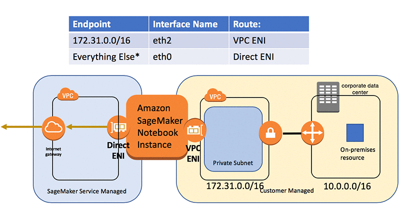
   In this configuration, all the traffic goes through the single network interface.  The notebook instance is running in an Amazon SageMaker managed VPC as shown in the above diagram.
2. Customer attached VPC with direct internet access (2 network interfaces)
   
   In this configuration, the notebook instance needs to decide which network traffic should go down either of the two network interfaces.
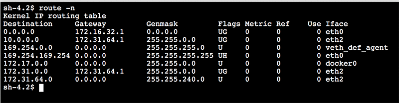
   If we look at an example where we launched into a VPC with a 172.31.0.0/16 CIDR range and look at the OS-level route information, we see this.
   
   Looking at this route table, we can see:
   • 172.31.0.0/16 traffic will use eth2 interface.
   • Some Docker and metadata routes.
   • All other traffic will use the eth0 interface.

   For simplicity, we’ll focus on the eth0 and eth2 configurations and not the other Docker/ec2 metadata entries. This shows us the following configuration:
   

   This default setting uses the internet network interface (eth0) for all traffic except for the CIDR range for the customer attached VPC (eth2). This setting sometimes needs to be overwritten when interacting with either on-premises or peered-VPC resources.

3. Customer attached VPC without direct internet access.
   IMPORTANT NOTE: In this configuration, the notebook instance can still be configured to access the internet. The network interface that gets launched only has a private IP address. What that means is that it needs to either be in a private subnet with a NAT or to access the internet back through a virtual private gateway. If launched into a public subnet, it won’t be able to speak to the internet through an internet gateway (IGW).
   

Common customer patterns

Accessing on-premises resources from an Amazon SageMaker instance with direct internet access:

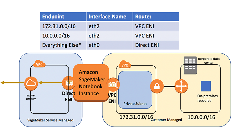
Suppose we have the following configuration:

If we try to access the on-premises resource in the 10.0.0.0/16 CIDR range, it will get routed by the OS through the eth0 internet interface. This interface doesn’t have the connection back on-premises and won’t allow us to communicate with on-premises resources.

To route back on premises, we’ll want to update the route table to have the following:

To do this, we can perform the following commands from a terminal on the Amazon SageMaker notebook instance:

Now if we look at the route table by entering “route -n” we see the route:

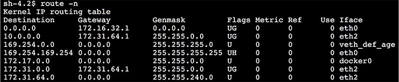
We see a route for 10.0.0.0 with mask 255.255.0.0 (which is the same as 10.0.0.0/16) going through the VPC routing IP address (172.31.64.1).

There is still one issue.

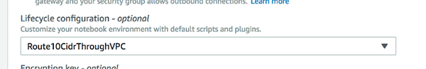
If we restart the notebook the changes won’t persist.  Only the changes made to the ML storage volume are persisted with a stop/start. Generally, for the package and files to be persisted, they need to be under “/home/ec2-user/SageMaker”. In this case, we’ll use a different feature: lifecycle configuration to add the route any time the notebook starts.

We can create a lifecycle policy as shown in the following diagram:

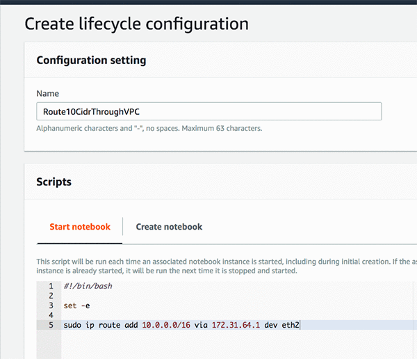
Now we can create our notebooks with this lifecycle configuration:

With this setup when the notebook gets created or when it’s stopped and restarted, we will have the networking configuration we expect:

Conclusion

Amazon SageMaker Jupyter notebooks are used to perform advanced data exploration, create model training jobs, deploy models to Amazon SageMaker hosting, and test or validate your models.  This drives the need for the notebook instances to have various networking configurations available to it.  Knowing how these configurations can be adapted allows you to integrate with existing resources in your organization and enterprise.

About the Author

Ben Snively is an AWS Public Sector Specialist Solutions Architect. He works with government, non-profit, and education customers on big data/analytical and AI/ML projects, helping them build solutions using AWS.

Amazon SageMaker now supports running Batch Transform jobs in Amazon Virtual Private Cloud (Amazon VPC) and using AWS Key Management Service (AWS KMS). Amazon VPC allows you to control access to your machine learning (ML) model containers and data so that they are private and aren’t accessible over the internet. AWS KMS enables you to encrypt data on the storage volume attached to the ML compute instances that run the Batch Transform job. This ensures that the model artifacts, logs, and temporary files used in your Batch Transform jobs are always secure. In this blog, I show you how to apply these features to Batch Transform jobs.

Amazon SageMaker Batch Transform is ideal for scenarios where you have large batches of data, need to pre-process and transform training data, or don’t need sub-second latency. You can use Batch Transform on a range of data sets, from petabytes of data to very small data sets. Existing machine learning models work seamlessly with this new capability, without any changes. Amazon SageMaker manages the provisioning of resources at the start of Batch Transform jobs. It then releases them when the jobs are complete, so you pay only for the resources used during the execution of the jobs.

Using a VPC helps to protect your model containers and the AWS resources they access such as the Amazon S3 buckets where you store your data and model artifacts because you can configure your VPC so that it is private and not connected to the internet. When you use a VPC, you can also monitor all network traffic in and out of your model containers by using VPC flow logs. If you don’t specify a VPC, Amazon SageMaker will run Batch Transform jobs in a VPC by default.

Amazon SageMaker Batch Transform already supports Amazon S3 SSE encryption of input and output data. Now, using AWS KMS, you can protect the storage volumes used during Batch Transform jobs with the encryption keys that you control. You can take advantage of AWS KMS features, such as centralized key management, key usage audit logging, and master key rotation, when you are running inferences or transforming batches of data. You can create, import, rotate, disable, delete, define usage policies for, and audit the use of encryption keys used to encrypt your data. AWS KMS is also integrated with AWS CloudTrail to provide you with logs of all key usage to help meet your regulatory and compliance needs.

How to create a Batch Transform job

Let’s take a look at how we run a Batch Transform job for the built-in Object Detection algorithm. I followed this example notebook to train my object detection model.

Now I’ll go to the Amazon SageMaker console and open the Models page to create a model and associate my private subnets and security groups.

From there I can create a model, using the object detection image and the model artifact generated from my training.

Here I name my model and specify the IAM role that provides the required permissions. Here I also specify the subnets and security groups in my private VPC to control access to my container and Amazon S3 data. As shown in the following screenshot, after I choose the VPC, Amazon SageMaker will auto-populate the subnets and security groups in that VPC. I have provided multiple subnets and security groups from my private VPC in this example. Amazon SageMaker Batch Transform will choose a single subnet to create elastic network interfaces (ENIs) in my VPC and attaches them to the model containers. These ENIs provide your model containers with a network connection so that my Batch Transform jobs can connect to resources in my private VPC without going over the internet.

Additionally, Amazon SageMaker will associate all security groups that I provide with the network interfaces created in my private VPC.

Separately, I have created a S3 VPC endpoint that allows my model containers to access the Amazon S3 bucket where my input data is stored, even if internet access is disabled. I recommend that you also create a custom policy that allows only requests from your private VPC to access to your S3 buckets. For more information, see Endpoints for Amazon S3.

I now proceed with specifying the inference container image Amazon Elastic Container Registry (Amazon ECR location) and the location of my model artifact from my object detection training job.

That’s it! We now have a model that is configured to run securely within a VPC.

Now, I will create a new Batch Transform job using the previously trained object detection model on the Selfies Dataset. Let’s go the Batch Transform page in the Amazon SageMaker console.

First, open the Amazon SageMaker console, choose Batch Transform, and choose Create Batch Transform job.

In the Batch Transform job configuration window, complete the form as shown in the following example. For more information about completing this form, see Using Batch Transform (Console)

Note that I have also specified the encryption key, using the new AWS KMS feature. Amazon SageMaker uses it to encrypt data on the storage volumes attached to the ML compute instances that run the Batch Transform job.

Next specify the input location. I can use either a manifest file or load all the files in an S3 location. Because I’m dealing with images, I specified my input content-type.

I also created a VPC endpoint that allows my model containers to access the Amazon S3 bucket where my input data is stored, even offline. I also recommend that you create a custom policy that allows requests only from your private VPC to access to your S3 buckets. For more information, see Endpoints for Amazon S3.

Finally, I’ll configure the output location and start the job, as shown in the following example. As mentioned before, you can specify a KMS encryption key for output, so that your Batch Transform outputs are encrypted server side with S3 KMS SSE.

After you start your transform job, you can open the job details page and follow the links to the metrics and the logs in Amazon CloudWatch.

Using Amazon CloudWatch, I can see that the transform job is running. If I look at my results in Amazon S3 I can see the predicted labels for each image, as shown in the following example:

The transform job creates a JSON file for each input file that contains the detected objects.

In your S3 bucket, it’s efficient to create a table for a bucket in AWS Glue. You then either query the results with Amazon Athena or visualize them using Amazon QuickSight.

It’s also possible to start transform jobs programmatically using the high-level Python library or the low-level SDK (boto3). For more information about how to use Batch Transform using your own containers, see Getting Inferences by Using Amazon SageMaker Batch Transform.

Batch Transform is ideal for use cases when you have large batches of data that need predictions, don’t need sub-second latency, or need to pre-process and transform training data. In this blog, we discussed how you can use Amazon VPC and AWS KMS to increase the security of your Batch Transform jobs. Amazon VPC and AWS KMS for Batch Transform are available in all AWS Regions where Amazon SageMaker is available. For more information, see the Amazon SageMaker developer guide.

About the Authors

Urvashi Chowdhary is a Senior Product Manager for Amazon SageMaker. She is passionate about working with customers and making machine learning more accessible. In her spare time, she loves sailing, paddle boarding, and kayaking.

Jeffrey Geevarghese is a Senior Engineer in Amazon AI where he’s passionate about building scalable infrastructure for deep learning. Prior to this he was working on machine learning algorithms and platforms and was part of the launch teams for both Amazon SageMaker and Amazon Machine Learning.

People are using Alexa for all types of activities in their homes, such as checking their bank balances, ordering pizza, or simply listening to their music from their favorite artists. For the most part, the primary interaction with the Echo has been your voice. In this blog post, we’ll show you how to build a new Alexa skill that will integrate with AWS DeepLens so when you ask “Alexa, what do you see?” Alexa returns objects detected by the AWS DeepLens device.

Object detection is an important topic in the AI deep learning world. For example, in autonomous driving, the camera on the vehicle needs to be able to detect objects (people, cars, signs, etc.) on the road first before making any decisions to turn, slow down, or stop.

AWS DeepLens was developed to put deep learning in the hands of developers. It ships with a fully programmable video camera, tutorials, code, and pre-trained models. It was designed so that you can have your first Deep Learning model running on the device within about 10 minutes after opening the box. For this blog post we’ll use one of the built-in object detection models included with AWS DeepLens. This enables AWS DeepLens to perform real-time object detection using the built-in camera. After the device detects objects, it sends information about the objects detected to the AWS IoT platform.

We’ll also show you how to push this data into an Amazon Kinesis data stream, and use Amazon Kinesis Data Analytics to aggregate duplicate objects detected in the stream and push them into another Kinesis data stream. Finally, you’ll create a custom Alexa skill with AWS Lambda to retrieve the detected objects from the Kinesis stream and have Alexa verbalize the result back to the user.

Solution overview

The following diagram depicts a high-level overview of this solution.

Amazon Kinesis Data Streams

You can use Amazon Kinesis Data Streams to build your own streaming application. This application can process and analyze real-time, streaming data by continuously capturing and storing terabytes of data per hour from hundreds of thousands of sources.

Amazon Kinesis Data Analytics

Amazon Kinesis Data Analytics provides an easy and familiar standard SQL language to analyze streaming data in real time. One of its most powerful features is that there are no new languages, processing frameworks, or complex machine learning algorithms that you need to learn.

AWS Lambda

AWS Lambda lets you run code without provisioning or managing servers. With AWS Lambda, you can run code for virtually any type of application or backend service – all with zero administration. Just upload your code and AWS Lambda takes care of everything required to run and scale your code with high availability. You can set up your code to automatically trigger from other AWS services or call it directly from any web app, mobile app, or, in this case, an Alexa skill.

Amazon Alexa

Alexa is the Amazon cloud-based voice service available on tens of millions of devices from Amazon and third-party device manufacturers. With Alexa, you can build natural voice experiences that offer customers a more intuitive way to interact with the technology they use every day. Our collection of tools, APIs, reference solutions, and documentation make it easy for anyone to build with Alexa.

Solution summary

The following is a quick walkthrough of the solution that’s illustrated in the diagram:

1. First set up the AWS DeepLens device and download the object detection model onto the device. Then it will load the model, perform local inference, and send detected objects as MQTT messages to the AWS IoT platform.
2. The MQTT messages are then sent to a Kinesis data stream by configuring an IoT rule.
3. By using Kinesis Data Analytics on the Kinesis data stream, detected objects are aggregated and put into another Kinesis data stream for the Alexa custom skill to query.
4. Upon the user’s request, the custom Alexa skill will invoke an AWS Lambda function, which will query the final Kinesis data stream and return list of objects detected by the AWS DeepLens device.

Implementation steps

The following sections walk through the implementation steps in detail.

Setting up DeepLens and deploying the built-in object detection model

1. Open the AWS DeepLens console.
2. Register your AWS DeepLens device if it’s not registered. You can follow this link for a step by step guide to register the device.
3. Choose Create new project on the Projects page. On the Choose project type page, choose the Use a project template option, and select Object detection in the Project templates section.
   
4. Choose Next to move to the Review
5. In the Project detail page, give the project a name and then choose Create.
6. Back on the Projects page, select the project that you created earlier, and click Deploy to device.
   
7. Make sure the AWS DeepLens device is online. Then select the device to deploy, and choose Review. Review the deployment summary and then choose Deploy.
8. The page will redirect to device detail page and at the top the page, deployment status is displayed. This process will take a few minutes, wait until the deployment is successful.
9. After the deployment is complete, on the same page, scroll to the device details section and copy the MQTT topic from AWS IoT that the device is registered to. As mentioned, any object detected by the AWS DeepLens device will send the information to this topic.
   
10. In the same section, choose the AWS IoT console link.
    
11. On the AWS IoT MQTT Client test page, paste the MQTT topic copied earlier and choose Subscribe to topic.
    

12. You should now see detected object messages flowing on the screen.

Setting up Kinesis Streams and Kinesis Analytics

1. Open the Amazon Kinesis Data Streams console.
2. Create a new Kinesis Data Stream. Give it a name that indicates it’s for raw incoming stream data—for example, RawStreamData. For Number of shards, type 1.
   
3. Go back to the AWS IoT console and in the left navigation pane choose Act. Then choose Create to set up a rule to push MQTT messages from the AWS DeepLens device to the newly created Kinesis data stream.
4. On the create rule page, give it a name. In the Message source section, for Attribute enter *. For Topic filter, enter the DeepLens device MQTT topic. Choose Add action.
   
5. Choose Sends message to an Amazon Kinesis Stream, then click Configuration action. Select the Kinesis data stream created earlier, and for Partition key type ${newuuid()} in the text box. Then choose Create a new role or Update role and choose Add action. Choose Create rule to finish the setup.
   
6. Now that the rule is set up, messages will be loaded into the Kinesis data stream. Now we can use Kinesis Data Analytics to aggregate the data and load the result to the final Kinesis data stream.
7. Open the Amazon Kinesis Data Streams console.
8. Create another new Kinesis Data Stream (follow instruction steps 1 and 2). Give it a name that indicates that it’s for aggregated incoming stream data—for example, AggregatedDataOutput. For Number of shards, type 1.
9. In the Amazon Kinesis Data Analytics console, create a new application.
   
10. Give it a name and choose Create application. In the source section, choose Connect stream data.
    
11. Select Kinesis stream as Source and select the source stream created in step 2. Choose Discover schema to let Kinesis Data Streams to auto-discover the data schema.
    
12. The Object Detection model deployment can detect up to 20 objects. However, AWS DeepLens might only detect a few of them depending on what’s in front of the camera. For example, in the screenshot below, the device only detects a chair and a person. Therefore, Kinesis auto discovery only detects the two objects as columns. You can add the other 18 objects manually to the schema by choosing the Edit schema button.
    
13. On the schema page, add the rest of the objects then choose Save schema and update stream. Wait for the update to complete then click Exit (done).
    
14. Scroll down to the bottom of the page then choose Save and continue.
15. Back on the application configuration page, choose Go to SQL editor.
16. Copy and paste the following SQL statement to the Analytics SQL window, and then choose Save and run SQL. After SQL finishes saving and running, choose Close at the bottom of the page. The SQL script aggregates each object detected in a 10 second tumbling window and stores them in the destination stream.

    CREATE OR REPLACE STREAM "TEMP_STREAM" ("objectName" varchar (40), "objectCount" integer);
    -- Creates an output stream and defines a schema
    CREATE OR REPLACE STREAM "DESTINATION_SQL_STREAM" ("objectName" varchar (40), "objectCount" integer);
     
    CREATE OR REPLACE PUMP "STREAM_PUMP_1" AS INSERT INTO "TEMP_STREAM"
    SELECT STREAM 'person', COUNT(*) AS "objectCount" FROM "SOURCE_SQL_STREAM_001"
    -- Uses a 10-second tumbling time window
    GROUP BY "person", STEP("SOURCE_SQL_STREAM_001".ROWTIME BY INTERVAL '10' SECOND);
    
    CREATE OR REPLACE PUMP "STREAM_PUMP_2" AS INSERT INTO "TEMP_STREAM"
    SELECT STREAM 'tvmonitor', COUNT(*) AS "objectCount" FROM "SOURCE_SQL_STREAM_001"
    -- Uses a 10-second tumbling time window
    GROUP BY "tvmonitor", STEP("SOURCE_SQL_STREAM_001".ROWTIME BY INTERVAL '10' SECOND);
    
    CREATE OR REPLACE PUMP "STREAM_PUMP_4" AS INSERT INTO "TEMP_STREAM"
    SELECT STREAM 'sofa', COUNT(*) AS "objectCount" FROM "SOURCE_SQL_STREAM_001"
    -- Uses a 10-second tumbling time window
    GROUP BY "sofa", STEP("SOURCE_SQL_STREAM_001".ROWTIME BY INTERVAL '10' SECOND);
    
    CREATE OR REPLACE PUMP "STREAM_PUMP_7" AS INSERT INTO "TEMP_STREAM"
    SELECT STREAM 'dog', COUNT(*) AS "objectCount" FROM "SOURCE_SQL_STREAM_001"
    -- Uses a 10-second tumbling time window
    GROUP BY "dog",  STEP("SOURCE_SQL_STREAM_001".ROWTIME BY INTERVAL '10' SECOND);
    
    CREATE OR REPLACE PUMP "STREAM_PUMP_10" AS INSERT INTO "TEMP_STREAM"
    SELECT STREAM 'chair', COUNT(*) AS "objectCount" FROM "SOURCE_SQL_STREAM_001"
    -- Uses a 10-second tumbling time window
    GROUP BY "chair",  STEP("SOURCE_SQL_STREAM_001".ROWTIME BY INTERVAL '10' SECOND);
    
    CREATE OR REPLACE PUMP "STREAM_PUMP_11" AS INSERT INTO "TEMP_STREAM"
    SELECT STREAM 'cat', COUNT(*) AS "objectCount" FROM "SOURCE_SQL_STREAM_001"
    -- Uses a 10-second tumbling time window
    GROUP BY "cat",  STEP("SOURCE_SQL_STREAM_001".ROWTIME BY INTERVAL '10' SECOND);
    
    CREATE OR REPLACE PUMP "STREAM_PUMP_14" AS INSERT INTO "TEMP_STREAM"
    SELECT STREAM 'bottle', COUNT(*) AS "objectCount" FROM "SOURCE_SQL_STREAM_001"
    -- Uses a 10-second tumbling time window
    GROUP BY "bottle", STEP("SOURCE_SQL_STREAM_001".ROWTIME BY INTERVAL '10' SECOND);
    
    CREATE OR REPLACE PUMP "OUTPUT_PUMP" AS INSERT INTO "DESTINATION_SQL_STREAM"
    SELECT STREAM "objectName", count(*) as "objectCount" FROM "TEMP_STREAM"
    GROUP BY "objectName", STEP("TEMP_STREAM".ROWTIME BY INTERVAL '10' SECOND)
    having count(*) >1;

17. Back on application configuration page, choose Connect to a destination. In the Analytics destination section, make sure the Kinesis data stream (for example, AggregatedDataOutput) created in step 8 is selected, and enter DESTINATION_SQL_STREAM as the In-application stream name and select JSON as the output format of. Note that you can also easily have Kinesis Data Analytics send data directly to a Lambda function. That Lambda function would write to other data stores, such as Amazon DynamoDB. Then have the Alexa read from DynamoDB upon user request.
    
18. Messages are now aggregated and loaded into the final Kinesis data stream (for example, AggregatedDataOutput) that was created in step 8. Next, you will create an Alexa custom skill with AWS Lambda.

Creating Alexa custom skill with AWS Lambda

1. Open the AWS Lambda console and create a new function.
2. The easiest way to create an Alexa skill is to create the function from the existing blue print provided by AWS Lambda and then overwrite the code with your own.
   
3. It is a security best practice to enable Alexa Skill ID when using a Lambda function. If you have not created a skill for this yet, you can disable it for now and then re-enable it later by adding another Alexa trigger to the Lambda function.
4. Copy the following Python code and replace the sample code provided by the blueprint. This code reads data from the Kinesis data stream and returns the result back to Alexa. Note: Change the default Northern Virginia AWS Region (us-east-1) in the code if you are following along in other Regions. Look for the following code to change region, kinesis = boto3.client(‘kinesis’, region_name=’us-east-1′)

   from __future__ import print_function
   import boto3
   import time
   import json
   import datetime   
   from datetime import timedelta
   
   def build_speechlet_response(title, output, reprompt_text, should_end_session):
       return {
           'outputSpeech': {
               'type': 'PlainText',
               'text': output
           },
           'card': {
               'type': 'Simple',
               'title': "SessionSpeechlet - " + title,
               'content': "SessionSpeechlet - " + output
           },
           'reprompt': {
               'outputSpeech': {
                   'type': 'PlainText',
                   'text': reprompt_text
               }
           },
           'shouldEndSession': should_end_session
       }
   def build_response(session_attributes, speechlet_response):
       return {
           'version': '1.0',
           'sessionAttributes': session_attributes,
           'response': speechlet_response
       }
   def get_welcome_response():
       """ If we wanted to initialize the session to have some attributes we could
       add those here
       """
   
       session_attributes = {}
       card_title = "Welcome"
       speech_output = "Hello, I can see now. You can ask me what I see around you right now."
       reprompt_text = "You can ask me what I see around you right now."
       should_end_session = False
       return build_response(session_attributes, build_speechlet_response(
           card_title, speech_output, reprompt_text, should_end_session))
   def handle_session_end_request():
       card_title = "Session Ended"
       speech_output = "Ok, I will close my eyes now. Have a nice day! "
       should_end_session = True
       return build_response({}, build_speechlet_response(
           card_title, speech_output, None, should_end_session))
   def create_object_names_attributes(objectNames, sequenceNumber):
       return {"objectNames": objectNames, "sequenceNumber":sequenceNumber}
   
   def get_objects(intent, session):
       session_attributes = {}
       reprompt_text = None
       speech_output=""
       should_end_session=False
       
       kinesis = boto3.client('kinesis', region_name='us-east-1')
       shard_id = 'shardId-000000000000'
       objectNames=[]
       sequenceNumber=""
   
       if session.get('attributes', {}) and "objectNames" in session.get('attributes', {}):
           objectNames = session['attributes']['objectNames']
       
       if session.get('attributes', {}) and "sequenceNumber" in session.get('attributes', {}):
               sequenceNumber = session['attributes']['sequenceNumber']
               
       if len(objectNames) ==0:
           if len(sequenceNumber)==0:   
               print("NO SEQUENCE NUMBER, GETTING OBJECTS DETECTED IN LAST FEW MINUTES")
               delta = timedelta(minutes=40)
               timestamp=datetime.datetime.now() - delta   
               shard_it = kinesis.get_shard_iterator(
                   StreamName='AggregatedDataOutput', 
                   ShardId=shard_id, 
                   ShardIteratorType='AT_TIMESTAMP',
                   Timestamp=timestamp)['ShardIterator']
           else:
               print("GOT SEQUENCE NUMBER, GETTING OBJECTS DETECTED - " + sequenceNumber)
               shard_it = kinesis.get_shard_iterator(
                   StreamName='AggregatedDataOutput', 
                   ShardId=shard_id, 
                   ShardIteratorType='AFTER_SEQUENCE_NUMBER',
                   StartingSequenceNumber=sequenceNumber)['ShardIterator']
                   
           while len(objectNames)<5:
               out = kinesis.get_records(ShardIterator=shard_it, Limit=2)
               shard_it = out["NextShardIterator"]
               if (len(out["Records"])) > 0:
                   theObject = json.loads(out["Records"][0]["Data"])
                   sequenceNumber = out["Records"][0]["SequenceNumber"]
                   #print ('sequenceNumber is ' + sequenceNumber)
                   objectName = theObject["objectName"]
                   objectCount = theObject["objectCount"]
                   if not (objectName in objectNames):
                       objectNames.append(objectName)
               else:
                   speech_output = "I currently do not see anything, is my deeplens on?"
                   break
               time.sleep(0.2)
               
       if len(objectNames) >0:
           objectName = objectNames[0]
           objectNames.remove(objectName)
           session_attributes = create_object_names_attributes(objectNames, sequenceNumber)
           speech_output = "I see " + objectName + "."
       print(speech_output)
   
       # Setting reprompt_text to None signifies that we do not want to reprompt
       # the user. If the user does not respond or says something that is not
       # understood, the session will end.
       return build_response(session_attributes, build_speechlet_response(
           intent['name'], speech_output, reprompt_text, should_end_session))
   
   # --------------- Events ------------------
   
   def on_session_started(session_started_request, session):
       """ Called when the session starts """
   
       print("on_session_started requestId=" + session_started_request['requestId']
             + ", sessionId=" + session['sessionId'])
   
   def on_launch(launch_request, session):
       """ Called when the user launches the skill without specifying what they
       want
       """
   
       print("on_launch requestId=" + launch_request['requestId'] +
             ", sessionId=" + session['sessionId'])
       # Dispatch to your skill's launch
       return get_welcome_response()
   
   def on_intent(intent_request, session):
       """ Called when the user specifies an intent for this skill """
   
       print("on_intent requestId=" + intent_request['requestId'] +
             ", sessionId=" + session['sessionId'])
   
       intent = intent_request['intent']
       intent_name = intent_request['intent']['name']
   
       # Dispatch to your skill's intent handlers
       if intent_name == "WhatDoYouSee":
           return get_objects(intent, session)
       elif intent_name == "AMAZON.HelpIntent":
           return get_welcome_response()
       elif intent_name == "AMAZON.CancelIntent" or intent_name == "AMAZON.StopIntent":
           return handle_session_end_request()
       else:
           raise ValueError("Invalid intent")
   
   def on_session_ended(session_ended_request, session):
       """ Called when the user ends the session.
   
       Is not called when the skill returns should_end_session=true
       """
       print("on_session_ended requestId=" + session_ended_request['requestId'] +
             ", sessionId=" + session['sessionId'])
       # add cleanup logic here
   
   # --------------- Main handler ------------------
   
   def lambda_handler(event, context):
       """ Route the incoming request based on type (LaunchRequest, IntentRequest,
       etc.) The JSON body of the request is provided in the event parameter.
       """
       print("event.session.application.applicationId=" +
             event['session']['application']['applicationId'])
   
       """
       Uncomment this if statement and populate with your skill's application ID to
       prevent someone else from configuring a skill that sends requests to this
       function.
       """
       # if (event['session']['application']['applicationId'] !=
       #         "amzn1.echo-sdk-ams.app.[unique-value-here]"):
       #     raise ValueError("Invalid Application ID")
   
       if event['session']['new']:
           on_session_started({'requestId': event['request']['requestId']},
                              event['session'])
   
       if event['request']['type'] == "LaunchRequest":
           return on_launch(event['request'], event['session'])
       elif event['request']['type'] == "IntentRequest":
           return on_intent(event['request'], event['session'])
       elif event['request']['type'] == "SessionEndedRequest":
           return on_session_ended(event['request'], event['session'])
   
   
   

Setting up an Alexa custom skill with AWS Lambda

1. Open the Amazon Alexa Developer Portal, and choose Create a new custom skill.
2. You can upload the JSON document in the Alexa Skill JSON Editor to automatically configure intents and sample utterances for the custom skill. Be sure to click Save Model to apply the changes.

   {
       "interactionModel": {
           "languageModel": {
               "invocationName": "deep lens demo",
               "intents": [
                   {
                       "name": "WhatDoYouSee",
                       "slots": [],
                       "samples": [
                           "anything else",
                           "do you see anything else",
                           "what else do you see",
                           "what else",
                           "how about now",
                           "what do you see around me",
                           "deep lens",
                           "what do you see",
                           "tell me what you see",
                           "what are you seeing",
                           "yes",
                           "yup",
                           "sure",
                           "yes please"
                       ]
                   },
                   {
                       "name": "AMAZON.HelpIntent",
                       "samples": []
                   },
                   {
                       "name": "AMAZON.StopIntent",
                       "samples": []
                   }
               ],
               "types": []
           }
       }
   }
   

   

3. Finally, in the endpoint section, enter the AWS Lambda function’s Amazon Resource Name (ARN) that’s created. Your Alexa Skill is set and ready to tell you the objects detected by the AWS DeepLens device. You can wake Alexa up by saying “Alexa, open Deep Lens demo” and then ask Alexa questions such as “What do you see?” Alexa should return an answer such as “I see a person” or “I see a chair,” etc.
   

Conclusion

In this blog post, you learned how to set up the AWS DeepLens device and deploy the built-in object detection model from the DeepLens console. Then, you could use AWS DeepLens to perform real-time object detection. Objects detected on the AWS DeepLens device were sent to the AWS IoT platform which then forwarded them to an Amazon Kinesis data stream. You also learned how to use Amazon Kinesis Data Analytics to aggregate duplicate objects detected in the stream and push them into another Kinesis data stream. Finally, you created a custom Alexa skill with AWS Lambda to retrieve the detected objects in the Kinesis data stream and return the result back to the users from Alexa.

About the authors

Tristan Li is a Solutions Architect with Amazon Web Services. He works with enterprise customers in the US, helping them adopt cloud technology to build scalable and secure solutions on AWS.

Grant McCarthy is an Enterprise Solutions Architect with Amazon Web Services, based in Charlotte, NC. His primary role is assisting his customers move workloads to the cloud securely and ensuring that the workloads are architected in way that aligns with AWS best practices.

Amazon Comprehend is a natural language processing (NLP) service that uses machine learning to find insights and relationships in text. The service does the following for you:

• Identifies the language of the text.
• Extracts key phrases, places, people, brands, or locations.
• Understands how positive or negative the text is.
• Analyzes text using tokenization and parts of speech.
• Automatically organizes a collection of text files by topic.

In today’s global marketplace, many companies require the ability to engage with their customers in a variety of languages, and Amazon Comprehend makes it easy to analyze those interactions. Today, we are pleased to announce that Amazon Comprehend supports four additional languages: French, German, Italian, and Portuguese. AWS customers can now analyze feedback and articles, and they can even organize information with native support for these languages.

Starting today, the service is also available in the AWS Europe (Frankfurt) Region. We also recently announced availability in the Asia Pacific (Sydney) Region. Amazon Comprehend continues to expand its regional availability enabling more AWS customers to analyze text in their native language, co-located with their data. To view an entire list of available Regions in which Amazon Comprehend is available, see our Region Table.

To get started, Comprehend provides a simple, no-code portal that allows customers to easily try the APIs with their own text, and now in additional languages. The following example shows the analysis of text containing named entities, in Italian, in the Amazon Comprehend console:

Amazon Comprehend provides synchronous and asynchronous APIs that allow you to analyze text based on the use cases that are best for your application. The following example shows a CLI call analyzing Italian text for the named entities:

Visit the AWS Management Console today to get started. Find out more information about free tier and pricing from this page.

About the Author

Woo Kim is a Product Marketing Manager for AWS machine learning services. He spent his childhood in South Korea and now lives in Seattle, WA. In his spare time, he enjoys playing volleyball and tennis.

AWS DeepLens is a deep-learning-enabled video camera for developers. It enables you to expand your deep learning skillsets through the use of a fully programmable video camera, tutorials, code, and pre-trained models.

The goal with this blog post is to show you how to get started with the AWS DeepLens and how this device facilitates the introduction of IoT and Deep Learning, putting it the hands of developers. In this blog post, we’ll show you how to build a simple face detection application that counts the number of cups of coffee that people drink and displays the tally on a leaderboard.

We will go through the following steps:

• Step 1: Deploy a sample project
• Step 2: Change the inference AWS Lambda function
• Step 3: Create a coffee detection backend
• Step 4: Deploy the app to AWS Elastic Beanstalk

Project Overview

Let’s review the following architectural diagram for the project. The AWS DeepLens device enables you to run deep learning on the edge. It detects a scene and runs it against a face detection model.

When the model detects a face, it uploads a frame to Amazon S3. An AWS Lambda function then runs the frame against AWS Rekognition to detect a mug in the scene and check if a face has been detected before or if is it a new face. After a face is registered or recognized, it’s stored in Amazon DynamoDB, which is used as an incremental counter for a web application.

Following this post, you’ll be able to replicate the architecture and get the necessary information to build an application like this.

Step 1: Deploy a sample project

To deploy the project you first need to register the AWS DeepLens device, if you haven’t already. See Register Your AWS DeepLens Device for more information.

• Go to the AWS DeepLens console and create a new project.

For the project type, make sure Use a project template is highlighted and select Face detection from the project templates.

From there you can specify the project name and add a description, leave everything else at the default, and choose Create.

2) After the project is created, we need to deploy it to the AWS DeepLens device. On the Projects page, select your project name, and then choose Deploy to device. On the target device page, select your registered AWS DeepLens device.

Choose Review.

After you have reviewed, finalize by choosing Deploy.

3) Navigate to the IAM console. Add permissions for AmazonS3FullAccess to AWSDeepLensGreengrassGroupRole.

Next you need to make sure that the project was successfully deployed. Connect the AWS DeepLens device to a monitor, mouse, and keyboard. Sign in to the device using the password that you set when you registered the device.

Start your terminal and run the following command:

mplayer —demuxer lavf -lavfdopts format=mjpeg:probesize=32 /tmp/results.mjpeg

This command shows the project stream. You will now see each frame being run against the model as the inference Lambda function is processed.

Step 2: Change the inference Lambda function

After you deploy the sample project, you need to change the inference Lambda function running on the device to upload images to Amazon S3. For this use case, we also added some messages on the screen to make the process more intuitive.

1) Create an Amazon S3 bucket where the images will be uploaded. Use the default settings when setting up the bucket and choose the same AWS Region as the rest of your infrastructure.

2) Go to the AWS Lambda console and open the deeplens-face-detection function. Remove the function code and replace it with the lambda_inference code here. (Replace the bucket_name variable with your bucket name.)

With this step, we are changing the code to upload images to Amazon S3 when a face is detected. Plus we are adding features such as a cooldown period between uploads and a countdown before taking a picture.

3) Save the AWS Lambda function and publish a new version of the code. This allows you to go to your AWS DeepLens project and update the function on the device.

Access your project in the AWS DeepLens console and edit the project updating the version of your AWS Lambda function and the timeout to 600 seconds:

4) Redeploy the project to the device by selecting the project and choosing Deploy.

You should also install botocore to the AWS DeepLens by using this command:

sudo -H pip install botocore

This allows the frame to be uploaded to S3.

Step 3: Create a coffee detection backend

To recognize faces, we will use Amazon Rekognition collections. A collection is a container for persisting faces detected by the IndexFaces API action. Amazon Rekognition doesn’t store copies of the analyzed images. Instead, it stores face feature vectors as the mathematic representation of a face within the collection.

You can use the facial information in a collection to search for known faces in images, stored videos, and streaming videos.

To create a collection you will first need to configure the AWS CLI:

1. Install the AWS CLI.
2. Configure the AWS CLI.

1) Create an empty Amazon Rekognition collection using this CLI command:

aws rekognition create-collection --collection-id "Faces" --region us-east-1 

2) Now, we are going to create an Amazon DynamoDB table for storing unique face feature vectors generated by Amazon Rekognition and the number of coffees each person had.

DynamoDB works well for this use case. As a fully managed service, you don’t need to worry about the elasticity and scalability of the database because there is no limit to the amount of data that can be stored in a DynamoDB table. As the size of the data set grows, DynamoDB automatically spreads the data over sufficient machine resources to meet storage requirements. If you weren’t using DynamoDB, the incremental count added to the table would require you to scale accordingly. As for pricing, with DynamoDB you only pay for the resources you provision. For this use case, though, it is quite possible to remain within the AWS Free Tier pricing model or have the project running at a low DynamoDB price point.

To create the table in DynamoDB, in the AWS Management Console, navigate to the DynamoDB console and create a table. Use Faces as the table name and faceID as the primary key, and leave the other settings as defaults.

We’ll also create a table named logs for storing the logs of your Lambda function. For this table use unixtime as the primary key.

3) Create an AWS Lambda function that calls Amazon Rekognition. First, go to the IAM console and create a role for AWS Lambda function. Apply the following managed policies to this role:

• AmazonRekognitionFullAccess
• AmazonDynamoDBFullAccess
• AmazonS3FullAccess
• AWSLambdaExecute

You should follow AWS IAM best practices for production implementations.

4) Finally, navigate to the Lambda console. Create a Lambda function with Python 3.6 as a runtime. Set the name of the S3 bucket that you configured before as your Lambda trigger. Configure the Event type, Prefix, and Suffix as shown in the following screenshot. This ensures that your Lambda function is triggered only when new .jpg objects that start with a key matching the images/ pattern are created within the bucket.

Replace the template Lambda code with the code you downloaded from GitHub. Modify the Lambda timeout to 1 minute.

Copy the code from the GitHub repository and paste in in the code box. Let’s inspect the Lambda code to understand what it’s doing:

  response = rekognition.detect_labels(Image=image, MaxLabels=123, MinConfidence=50)    
    for object in response["Labels"]:
        if object["Name"] == "Coffee Cup" or object["Name"] == "Cup":
            coffee_cup_detected = True
            break        
            ::
        message = detect_faces(image, bucket, key)    

This part of code uses AWS Rekognition to detect the labels in the image. It checks if “Cup” or “Coffee Cup” is found in a response. If it finds any of these labels, it calls a face detection function, which searches the face collection to find if there is a matching face:

faces = rekognition.search_faces_by_image(CollectionId=face_collection, Image=image,
                                              FaceMatchThreshold=face_match_threshold, MaxFaces=1)

If no matching faces are found in the collection, the face is indexed and added to the collection:

faces = rekognition.index_faces(Image=image, CollectionId=face_collection)

To test the function, you can upload an image to your S3 bucket and check your DynamoDB table to see the result.

Step 4: Deploy the app to AWS Elastic Beanstalk

Now it’s time to deploy the leaderboard application using AWS Elastic Beanstalk. Elastic Beanstalk automatically orchestrates the required resources needed to deploy the web application. All you have to do is upload the code.

1) Go to the IAM console, and on the IAM roles page, attach the AmazonS3FullAccess and DynamoDBFullAccess managed policies to the aws-elasticbeanstalk-ec2-role. This allows Amazon EC2 instances provisioned by Elastic Beanstalk to access Amazon S3 and Amazon DynamoDB.

2) Go to the AWS Elastic Beanstalk console, and create a new application. Create a new web server environment. Enter a domain name, select Python as a platform, and upload a ZIP file from GitHub that includes the Flask application and requirements.txt file. Wait until Elastic Beanstalk provisions your environment.

The URL of your application should be visible on the top of your screen. Click the URL to view your coffee leaderboard!

Important: Deploying a project incurs costs for the various AWS services that are used.

Conclusion

You are now able to track the number of coffees each individual person drinks. While this project focuses on a simple coffee leaderboard, the backbone of this architecture can be used for any application.

This project showcases the power of the AWS DeepLens device in introducing developers to machine learning and IoT. Using a combination of AWS services, we were able to build this app in a short amount of time, and so can you!

About the Authors

João Coelho is a Solutions Architect at Amazon Web Services in London. He helps customers leverage the AWS platform to build scalable and resilient architectures on the cloud and is especially interested in serverless technologies. Outside of work, he enjoys playing tennis and traveling.

Laurynas Tumosa is a Technical Researcher at AWS in London. He enjoys building on the platform using AWS Machine Learning Services. He is passionate about making AI technologies accessible for everyone. Outside of work, Laurynas enjoys finding new interesting podcasts, playing guitar, and reading.

Lalit Dayalani is a Solution Architect at Amazon Web Services based in London. He helps AWS customers to provide guidance and technical assistance helping them understand and improve the value of their solutions on AWS. In his spare time, he loves spending time with family, going on hikes and spends way too much time indulging in too much television.

Retailers have been using in-store video to analyze customer behaviors and demographics for many years.  Separate systems are commonly used for different tasks.  For example, one system would count the number of customers moving through a store, in which part of the store those customers linger and near which products.  Another system will hold the store layout, whilst yet another may record transactions.  Historically, for a retailer to join these data sources to gain insights which could drive more sales by following a strategy has required complex algorithms and data structures that also require significant investment to deliver and incur ongoing maintenance costs.

In this blog post, we will demonstrate how to simplify this process using AWS services (Amazon Rekognition, AWS Lambda, Amazon S3, AWS Glue, AWS Athena and AWS QuickSight) to build an end-to-end solution for in-store video analytics. We will focus on the analysis of still images leveraging an existing loss prevention store camera to produce data for the retail in-store experience.

The following diagram shows the overall architecture and the AWS services involved.

Using the Machine Learning services on AWS like Amazon Rekognition and applying them to motion video or still images from your store, it is possible to derive insights from customer behavior (i.e. which area of the store is frequently visited), demographic segmentation of store traffic (i.e. such as gender or approximate age) while also analyzing patterns of customer sentiment. This practice is already common in the industry, and our proposed solution makes it easier, faster, and more accurate. Sentiment analysis can be used, for example, to get insights into how customers respond to brand content and signage, end cap displays or advertising campaigns while presenting these insights using dashboards similar to the examples shown below.

The overall solution can be decomposed into four main steps, collect, store, process and analyze.  Let’s describe each of these components:

Collect

The purpose of this stage is to collect images or motion video of your customers in-store experience from the camera.   This is possible by making use of various cameras such as an existing CCTV or IP Camera system, a (configured) Raspberry Pi with an attached camera module, an AWS DeepLens,  or any other similar camera.   These still images or motion video files are stored in an Amazon S3 bucket for further processing.

For this example, we used a Raspberry Pi with the motion package installed. This package helps to collect images when there is an interesting event that limits the amount of data needed to be processed. This package also detects motion, creates still images in a local folder, and this folder can be easily synced (in a realtime or batch manner) to the input S3 bucket. After installing the AWS Command Line (instructions here), here is one example of syncing the motion folder to an S3 bucket and deleting locally the file after successful synchronisation (need to adapt the destination bucket to your specific bucket).

aws s3 sync /var/lib/motion/ s3://retail_instore_demo_source/`hostname` && sudo find /var/lib/motion/ -type f -mmin +1 -delete

Store

We propose using Amazon S3 object store so we can benefit from its virtually unlimited storage, high availability and event triggering capabilities.  After creating this bucket, we enable the Amazon S3 event notification capability to publish events to AWS Lambda for every new file in the input folder, then an invoked Lambda function will pass the event data (i.e., incoming data as a parameter to be processed).

Process

To process the incoming images, we use AWS Lambda to read the image and use the Amazon Rekognition APIs to gather all of the relevant information provided by Rekognition for each image (such as facial landmarks that include the coordinates for eye and mouth), gender, age, presence of beard, sunglasses etc) and put the resulting information to a Amazon Kinesis Data Firehose which will publish the data to an Amazon S3 bucket. Amazon Kinesis Data Firehose simplifies the data management because it automatically handles the encryption, the folder structure (year/month/day/hour), optional data transformation, and compression.

The resulting dataset is a set of JSON files that contain the output from Rekognition, representing customers captured on these images. For effective querying from S3 we recommend the files to be in columnar format. One option is to use Amazon Firehose data Data Transformation feature, another is to convert the JSON using AWS Lambda or AWS Glue. Querying small datasets of JSON files is fine but as the table grows with thousands of files it will become less optimal. In this demo, we will be using JSON format to keep it simple.

Analyze

All the resulting information is then stored in a new Amazon S3 bucket.   Per the process step, the information is stored in a JSON format and therefore allows to be queried with Amazon Athena.  Therefore we can use AWS Glue Crawlers to automatically infer the data schema based on the data sitting in S3 and use the shared AWS Glue Catalog for Amazon Athena to query the data.  Amazon Athena is a service that allows you to query data directly in S3 using standard ANSI SQL commands and without needing to spin up any infrastructure.  This allows any data visualization / dashboard tool (i.e. Tableu, Superset, or Amazon QuickSight) to connect to Athena and visualize the data.  For our example, we will show how we can use Amazon QuickSight to create a dashboard for this data.

Build this solution yourself

Now that we have described the components of this solution, let’s bring it all together.

We have provided a CloudFormation template which will deploy all the necessary components shown in the architecture diagram except Amazon QuickSight and also the devices IP Camera / Raspberry Pi.  In the following section, we will explain key parts of the solution and show how we can make sense of all the analyzed data using Amazon QuickSight while building the dashboard manually.

Note: Cloud Formation template is tested only on eu-west-1 (Ireland) region and it may not work in other regions. Some of the resources deployed by the stack incur costs as long as they’re in use.

To get started deploying the CloudFormation template, take these steps:

1. Choose the Launch Stack button. It automatically launches the AWS CloudFormation service in eu-west-1 region on your AWS account with a template. You’re prompted to sign in if needed.
   

   Input	Value
   Region	eu-west-1
   CFN Template	https://s3-eu-west-1.amazonaws.com/retail-instore-analysis/retail-instore-demo-cloudformation.json

2. Choose Next to proceed with the following settings.
   
3. Specify the name of the CloudFormation stack and the required parameters. The default bucket name on the template might have been used, please change the bucket names to a unique name and click Next.
   

   	A	B
   1	Parameter	Description
   2	SourceBucketName	Unique bucket name where the images files will be uploaded for processing
   3	ProcessedBucketName	Unique bucket name where the processed files will be stored
   4	ArchivedBucketName	Unique bucket name where the images files will be archived after processing

   

4. On the Review page, acknowledge that CloudFormation creates AWS Identity and Access Management (IAM)resources and with custom names as a result of launching the stack.
5. Custom names are required because the template uses serverless transforms. Choose Create Change Set to check the resources that the transforms add, then choose Execute.
   
6. After the CloudFormation stack is launched, wait until the status changes from CREATE_IN_PROGRESS to CREATE_COMPLETE. Usually it takes around 7 to 9 minutes to provision all the required resources.
   
7. When the launch is finished, you’ll see a set of resources that we’ll use throughout this blog post:
   

Test the functionality

Once AWS CloudFormation template has created the required resources, lets use some pre-captured sample images to process, and AWS Glue crawlers to automatically discover the schema of our processed image data.

1. Download the pre-captured images from the S3 bucket https://s3-eu-west-1.amazonaws.com/retail-instore-analysis/Amazon_Fresh_Pickup_Images.zip
2. Open the source bucket (retail-instore-demo-source), and upload an image or multiple images with multiple people in it. For this example, use few of the downloaded images from the step 1 as you could upload other images later each hour to get different time interval graphs.
3. Lambda will be triggered, image analyzed using Amazon Rekognition and the results will be put in the S3 processed bucket (retail-instore-demo-processed) for further processing by Athena and QuickSight. You can monitor the files being processed either by watching the processed images being dropped in the processed bucket or by monitoring the AWS Lambda executions in the Lambda Monitoring Console.
4. In order to query using Athena, first we need to create the tables. We will leverage the AWS Glue crawlers which will automatically discover the schema of our data and create the appropriate table definition in AWS Glue Data Catalog. More details can be found in the documentation for Crawlers with AWS Glue.

By launching a stack from the CloudFormation template, we have only created a Crawler and configured it to “run on demand” as it’s charged hourly. Therefore, we need to run the Crawler manually when we have new data sources to construct the data catalog using pre-built classifiers. To do this, Go to AWS Glue, under Crawlers, run the crawler (retail-instore-demo-glue-s3-crawler).

The Crawler connects to the S3 bucket, progresses through a prioritized list of classifiers to determine the schema for your data, and then creates metadata tables in AWS Glue Data Catalog which will be used to query the processed content in S3 using Athena on top of which we will build a QuickSight dashboard.

Note: Make sure you upload pictures at different time and repeat step 2 to 4, so that you can see graph projection at different timelines.

Building QuickSight dashboards

First let’s the configure the QuickSight with the dataset.

1. Login into the QuickSight console – https://eu-west-1.quicksight.aws.amazon.com/sn/start
2. If it’s the first time you access QuickSight, follow the instruction below. If not, go to step 3.
   1. click on “Sign up for QuickSight”
   2. select the “Standard” edition
   3. Enter a QuickSight Account name
   4. Enter a valid Email
   5. Select the EU (Ireland) Region
   6. Tick the checkbox next to “Amazon Athena”
   7. Tick the checkbox next to “Amazon S3”
   8. click “choose s3 buckets” and select the retail_instore_demo_processed bucket
3. Choose Manage data from the top right.
4. Choose New Data Set.
5. Create a Data Set from Athena Data Source as “retail-instore-analysis-blog”
6. Choose the “retail-instore-demo-db” database, select the “retail_instore_demo_processed” table and click on Select
   
7. Leave it on default Import to SPICE for quicker analytics and then click Visualize.
8. Import complete will appear with the total rows imported to SPICE (which is the in-memory storage component used by QuickSight)Now you can easily start to build some dashboards. We will step through creating a dashboard.
9. We will first add a custom date field, so that we can have graphs with time axis. Click on “Add” and Add calculated field.
   
10. Provide a name for the Calculated field name like “DateCalculated”
11. Select “epochDate” from Function list, select “retailtimestamp” from Fieldlist, and Create.
    
    
12. This should create the calculated field.
13. Resize the visual windows as necessary, and select “Vertical stacked bar chart” under Visual types.
14. From Fields list, drag and drop the “DateCalculated” to X axis, “emotion” to Value and “emotion” to Group/Color on the Field wells. Graph will be populated based on the emotions captured from the images.
15. Click on drop down arrow on “DateCacluated” in X axis of Field wells, and scroll over “Aggregate: Day” and select “Hour”
16. This graph will display the emotions of people in different timestamps. For example, this can be a dashboard to display emotions captured at Aisle 23 while tracking a new product response on that aisle.  Another example, this allows to better count and qualify customers in front of a specific store endcap.
17. Lets add few more visuals. Click on “Add” and Add visual.
    
18. Select “pie chart” from Visual types and drag and drop “emotion” from fields list to Group/Color on Field wells
    
19. You can further enrich you dashboard by adding meaningful heading, and also adding other visual types with fields list as below,

• add a new Visual, Select “Vertical bar char”, Set X axis as DateCalculated(DAY), Value as emotion(count) in Field wells:
  

Results

The QuickSight dashboard above shows analysis of image capture events in a store.  For examples, you can see analysis of overall customer sentiment. You could understand the customer age range, and how many people visited each day from these metrics. Once you’re done with your analysis, you can easily share these insights with others in your team or organization by publishing it as a dashboard.

Using Amazon Rekognition you can better segment your customers.  You can obtain feedback on customer experience for a specific area of the store.

Shutting down

When you have finished experimenting, you can remove all the resources by following these steps.

1. Delete the contents inside all the S3 buckets that the CloudFormation template created.
2. Delete the CloudFormation stack.

Conclusions and next steps

This post showed you how simple it is to gain insights into customers’ in-store behaviour using AWS. Using your existing cctv systems or any camera, you can quickly build this solution and adapt it to your needs.

Some additional concepts that leverage this solution are:

• In-store video streams analysis:Using Kinesis Videostreams it’s possible to stream your existing videos, which allows for additional use cases such as capturing the path of customers (and using heatmaps) and where they spent time in the store.
• Customer loyalty and engagement programs utilizing facial recognition: Another very interesting possibility is the ability to recognize customers who have opted-in and shared a profile photo of themselves as part of a loyalty program, incentive program, or other customer benefit. Using the volunteered data, those customers could be recognized and offered a more elevated and personalized customer experience at a retail location.

If you have questions or suggestions, please comment below.

Additional Reading

• Use facial recognition to deliver high-end consumer experience
• Optimize the data using Apache Parquet

About the Authors

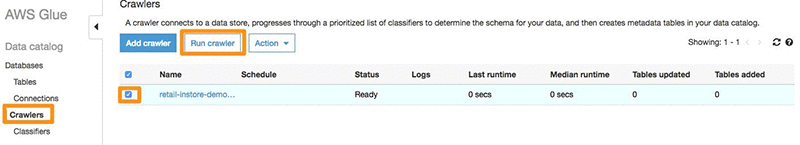
Bastien Leblanc is a Solutions Architect with AWS. He helps Retail customers adopt the AWS Platform, focusing on Data & Analytics workloads, he likes to work with customers helping to solve retail problems and drive innovation.

Imran Dawood is a Solutions Architect with AWS. He works with Retail customers helping them build solutions on AWS with architectural guidance to achieve success in the AWS cloud. In his spare time, Imran enjoys playing table tennis and spending time with family.

Amazon SageMaker now comes with a faster Pipe mode implementation, significantly accelerating the speeds at which data can be streamed from Amazon Simple Storage Service (S3) into Amazon SageMaker while training machine learning models.

Pipe mode offers significantly better read throughput than the File mode that downloads data to the local Amazon Elastic Block Store (EBS) volume prior to starting the model training. This means your training jobs start sooner, finish quicker, and need less disk space, reducing your overall cost to train machine learning models on Amazon SageMaker. For example, we conducted internal benchmarks earlier this year when we launched Pipe Input Mode for Amazon SageMaker built-in algorithms. We learned that start times were reduced by up to 87 percent on a 78 GB training dataset. In addition, we saw that throughput was twice as fast in some benchmarks, resulting in up to 35 percent reduction in total training time.

Overview

Amazon SageMaker supports two mechanisms for transferring training data: File mode and Pipe mode. In File mode, the training data is downloaded first to an encrypted EBS volume attached to the training instance prior to commencing the training. However, in Pipe mode the input data is streamed directly to the training algorithm while it is running. This continuous streaming of data enables a few significant advantages. First, the startup time of a training job becomes independent of the size of the input data, resulting in much quicker startup, especially while training on gigabyte- and petabyte-scale datasets. Furthermore, you don’t have to pay for a large disk volume to download large datasets. Finally, if your training algorithm is I/O-bound, the highly concurrent, high-throughput reading mechanism employed by Pipe mode can significantly speed up your model training.

Higher I/O throughput with faster Pipe mode

The latest implementation of Pipe mode provides higher data streaming throughputs than before. The following chart demonstrates the throughput improvements in Pipe mode compared to when we launched Pipe mode support earlier this year. For apples to apples comparison, the streaming throughput numbers are baselined against that of File mode as measured across instance types supported by Amazon SageMaker training.

As you can see, streaming training data using Pipe mode is now up to three times faster than before in some cases. Pipe mode support is available out of the box for Amazon SageMaker built-in algorithms. Now we will present an example of how you can take advantage of the Pipe mode if you are bringing your own custom training algorithms to Amazon SageMaker.

Writing Pipe mode training code

In Pipe mode, data is pre-fetched from Amazon S3 at high-concurrency and throughput and streamed into Unix Named Pipes (aka FIFOs). There is one FIFO per channel per epoch. The algorithm must open the FIFO for reading and read through to <EOF> (or optionally abort mid-stream). It must close its end-of-the-file descriptor when done. It can then optionally wait for the next epoch’s FIFO to get created and then it can commence reading. The algorithm iterates through epochs until achieves its completion criteria.

This notebook example has an extremely simple Pipe mode “training” algorithm implementation in Python. It conforms to the specifications required by Amazon SageMaker training It reads data in Pipe mode but does nothing with the data. It simply reads it and throws it away. The example is written this way to illustrate exactly what’s needed to support Pipe mode without complicating the code with a real training algorithm.

The train.py Python program contains the code. The following code snippet iterates through reading each epoch’s data through its corresponding FIFO:

# We're allocating a byte array here to read data into; a real algorithm
# may opt to prefetch the data into a memory buffer and train
# in parallel so that both IO and training happen simultaneously
data = bytearray(16777216)
total_read = 0
total_duration = 0
for epoch in range(num_epochs):
    check_termination()
    epoch_bytes_read = 0
    # As per the Amazon SageMaker training spec, the FIFO's path will be based on
    # the channel name and the current epoch:
    fifo_path = '{0}/{1}_{2}'.format(data_dir, channel_name, epoch)

    # Usually the FIFO will already exist by the time we get here, but
    # to be safe we should wait to confirm:
    wait_till_fifo_exists(fifo_path)
    with open(fifo_path, 'rb', buffering=0) as fifo:
        print('opened fifo: %s' % fifo_path)
        # Now simply iterate reading from the file until EOF. Again, a
        # real algorithm will actually do something with the data
        # rather than simply reading and immediately discarding like we
        # are doing here
        start = time.time()
        bytes_read = fifo.readinto(data)
        total_read += bytes_read
        epoch_bytes_read += bytes_read
        while bytes_read > 0 and not terminated:
            bytes_read = fifo.readinto(data)
            total_read += bytes_read
            epoch_bytes_read += bytes_read

        duration = time.time() - start
        total_duration += duration
        epoch_throughput = epoch_bytes_read / duration / 1000000
        print('Completed epoch %s; read %s bytes; time: %.2fs, throughput: %.2f MB/s'
              % (epoch, epoch_bytes_read, duration, epoch_throughput))

Using Pipe mode versus File mode

There are a few situations where Pipe mode may not be the optimum choice for training. In that case you should stick to using File mode:

• If your algorithm needs to backtrack or skip ahead within an epoch. This isn’t possible in Pipe mode because the underlying FIFO cannot support lseek() operations.
• If your training dataset is small enough to fit in memory and you need to run multiple epochs. In this case it might be quicker and easier just to load it all into memory and iterate.
• If it is not easy to parse your training dataset from a streaming source.

In all other scenarios, if you have an I/O-bound training algorithm, switching to Pipe mode should give you a significant throughput-boost as well as reduce the size of the disk volume required. This should result in both saving you time and reducing training costs.

About the authors

Ishaaq Chandy is a Senior Engineer in Amazon AI where he loves his work in building an innovative and massively scalable training platform for Amazon Sagemaker. Prior to this he was working on AWS ELB where he was part of the launch teams for both ALB as well as NLB.

Sumit Thakur works on products that make it quick and easy for customers to get started with deep learning on cloud. He is product manager for Amazon SageMaker and AWS Deep Learning AMI. In his spare time, he likes connecting with nature and watching sci-fi TV series.

In this blog post, we introduce three new features of the Amazon SageMaker Neural Topic Model (NTM) that are designed to help improve user productivity, enhance topic evaluation capability, and speed up model training. In addition to these new features, by optimizing sparse operations and the parameter server, we have improved the speed of the algorithm by 2x for training and 4x for evaluation on a single GPU. The speedup is even more significant for multi-GPU training.

Amazon SageMaker NTM is an unsupervised learning algorithm that learns the topic distributions of large collections of documents (corpus). With SageMaker NTM, you can build machine learning solutions for use cases such as document classification, information retrieval, and content recommendation. See Introduction to the Amazon SageMaker Neural Topic Model if you aren’t already familiar with Amazon SageMaker NTM.

If you are new to machine learning, or want to free up time to focus on other tasks, then the fully automated Amazon Comprehend topic modeling API is your best option. If you are a data science specialist looking for finer control over the various layers of building and tuning your own topic modeling model, then the Amazon SageMaker NTM might work better for you. For example, let’s say you are building a document topic tagging application that needs a customized vocabulary, and you need the ability to adjust the algorithm hyperparameters, such as the number of layers of the neural network, so you can train a topic model that meets the target accuracy in terms of coherence and uniqueness scores. In this case, the Amazon SageMaker NTM would be the appropriate tool to use.

Auxiliary vocabulary channel

When training a topic model, it’s important to know the top words in each of the topics so customers can understand what a topic is about. For customers who want to retrieve the actual representation of the words for each of the topics instead of integer representations from an Amazon SageMaker NTM model, they can now use the auxiliary vocabulary channel feature to remove the manual mapping effort.

Currently, when an Amazon SageMaker NTM training job runs, it outputs the training status and evaluation metrics to Amazon CloudWatch Logs and directly inside the Jupyter console. Among the outputs are lists of top words for the different topics detected. Prior to the availability of auxiliary vocabulary channel support, the top words were represented as integers, and customers needed to map the integers to an external custom vocabulary lookup table in order to know what the actual words were. With the support of the auxiliary vocabulary channel, users can now add a vocabulary file as an additional data input channel, and Amazon SageMaker NTM will output the actual words for a topic instead of integers. This feature eliminates the manual effort needed to map integers to the actual vocabulary. The following sample shows what a custom vocabulary text file looks like. The text file simply contains a list of words, one word per row, in the order corresponding to the integer IDs provided in the data.

absent
absentee
absolute
absolutely

To include an auxiliary vocabulary for a training job, you should name the vocabulary file vocab.txt and place it in the auxiliary directory. See the following sample code for the syntax for adding auxiliary vocabulary file. UTF-8 encoding is supported for the vocabulary file.

# s3_aux_data contains the auxiliary channel path on s3. E.g. "s3://bucketname/auxiliary"
s3_aux = s3_input(s3_aux_data, distribution='FullyReplicated', content_type='text/plain')
s3_train = s3_input(s3_train_data, distribution='ShardedByS3Key',
                    content_type='application/x-recordio-protobuf')
s3_val = s3_input(s3_val_data, distribution='FullyReplicated',
                  content_type='application/x-recordio-protobuf')
ntm.fit({'train': s3_train, 'validation': s3_val, 'auxiliary': s3_aux})

After the training is completed, the output looks like the following:

[09/07/2018 12:55:38 INFO 139989295474496] Topics from epoch:final (num_topics:20) [wetc 0.37, tu 0.75]:
[09/07/2018 12:55:38 INFO 139989295474496] [0.39, 0.72] game season september released power episode novel player ign jack playstation career trek boy life caused music people death fan
[09/07/2018 12:55:38 INFO 139989295474496] [0.31, 0.75] single hit design tube speed tropical maximum final nuclear storm mm taxonomy drum peaked depth wave reached wind lb iii
[09/07/2018 12:55:38 INFO 139989295474496] [0.35, 0.65] died record recorded st highway ny rule intersection chart intersects connector house century reached death billboard route charter king sr
[09/07/2018 12:55:38 INFO 139989295474496] [0.42, 0.77] gameplay player game battalion group division goal league mode match win football infantry score japanese attack regular enemy defeating yard
[09/07/2018 12:55:38 INFO 139989295474496] [0.38, 0.74] creek century mile water completed construction battalion freeway river destroyer interchange operation highway foot service city tower intersection cambridge gun
[09/07/2018 12:55:38 INFO 139989295474496] [0.36, 0.83] stone personnel film built chart long song sr rock album hop certification u rolling listing provided carey instrument instrumentation single
[09/07/2018 12:55:38 INFO 139989295474496] [0.37, 0.83] description forest possession era straight century remains round record existed yellow semi current county goal designation latin east hindu age
[09/07/2018 12:55:38 INFO 139989295474496] [0.40, 0.73] novel u bishop king archbishop fiction state poem god story henry cathedral expressed entire church new change originally turn force
[09/07/2018 12:55:38 INFO 139989295474496] [0.33, 0.73] game gameplay star race tournament body episode series developer unit player ha leslie character announced ray session international staff andy
[09/07/2018 12:55:38 INFO 139989295474496] [0.43, 0.86] team season game competition appearance florida play ground level brown japan goal summer host australia flight live feature specie injury
[09/07/2018 12:55:38 INFO 139989295474496] [0.35, 0.70] personnel surrender heavy reached radio single party bishop hit wave ship british parliament territory mm gun robert equipment issued armament
[09/07/2018 12:55:38 INFO 139989295474496] [0.41, 0.80] line french german zealand club race poem men force class light british position african american boat share smith veronica crew
[09/07/2018 12:55:38 INFO 139989295474496] [0.40, 0.83] simpson million development network map percent female doe level volume police people park developed water production business company public begin
[09/07/2018 12:55:38 INFO 139989295474496] [0.33, 0.70] game hill manchester building player division train battalion church oslo elected film vote baltimore amateur seat gate regiment infantry borough
[09/07/2018 12:55:38 INFO 139989295474496] [0.38, 0.63] ship water wind caused storm homer people poem hour affected line episode movement effect developed viewer house burn death street
[09/07/2018 12:55:38 INFO 139989295474496] [0.35, 0.82] raaf battalion party political building command rebel unit emperor hm granted outbreak brigade army restaurant cambridge appointed squadron commanded church
[09/07/2018 12:55:38 INFO 139989295474496] [0.30, 0.85] painting pagan century wasp altar architecture medieval church mary archaeologist era settlement witchcraft breed ode centre shakespeare religious scholar creek
[09/07/2018 12:55:38 INFO 139989295474496] [0.40, 0.70] episode season black series star aired character film female dvd speed rating nielsen simpson plot writer nbc director producer game
[09/07/2018 12:55:38 INFO 139989295474496] [0.41, 0.68] government community killed force vote archbishop turned death house dublin scholar legislation continued died opposed god king existed county official
[09/07/2018 12:55:38 INFO 139989295474496] [0.31, 0.70] class draft season assigned defense touchdown route ton division decommissioned line destroyer fleet mm torpedo boat tube sister king battleship

Word embedding topic coherence metric

To evaluate the performance of a trained Amazon SageMaker NTM model, customers can examine the perplexity metric emitted by a training job. Another measure of model quality is the semantic similarity of top words in each topic. A high-quality model should have words that are semantically similar in each of topics. For customers who want to effectively measure the topic coherence during training, they can now use the new word embedding topic coherence (WETC) feature.

Traditional methods like normalized point-wise mutual information (NPMI), while widely accepted, require a large external corpus. The new WETC metric measures the similarity of words in a topic by using a pre-trained word embedding, Glove-6B-400K-50d.

Intuitively, each word in the vocabulary is given a vector representation (embedding). We compute the WETC of a topic by averaging the pair-wise cosine similarities between the vectors corresponding to the top words of the topic. Finally, we average the WETC for all the topics to obtain a single score for the model.

Our tests have shown that WETC correlates very well with NPMI as an effective surrogate. For details about the pair-wise WETC computation and its correlation to NPMI, please refer to our paper [1]

WETC value ranges between 0 and 1, the higher value indicates a higher degree of topic coherence. A typical value would be in the range of 0.2 to 0.8. The WETC metric is evaluated whenever the vocabulary file is provided. The average WETC score over the topics is displayed in the log above the top words of all topics. The WETC metric for each topic is also displayed along with the top words of each topic. See the following screenshot for an example.

Note: In the situation in which many of the words in the supplied vocabulary can’t be found in the pre-trained word embedding, the WETC score can be misleading. Therefore, we provide a warning message to alert the user to exactly how many words in the vocabulary do not have an embedding:

[09/07/2018 14:18:57 WARNING 140296605947712] 69 out of 16648 in vocabulary do not have embeddings! Default vector used for unknown embedding!

Topic uniqueness metric

A good topic modeling algorithm should generate topics that are unique to avoid topic duplication. Customers who want to understand the topic uniqueness of a trained Amazon SageMaker NTM model to evaluate its quality can now use the new topic uniqueness (TU) metric.

To understand how TU works, suppose there are K topics, and we extract the top n words for each topic. The TU for topic k is defined as:

where cnt(i,k) is the total number of times the ith top word in topic k appears in the top words across all topics. E.g. if the ith top word in topic k appears only in topic k, then cnt(i,k)=1; on the other hand, if the word appears in all the topics then cnt(i,k)=K. Finally, the average TU is computed as:

The range of the TU value is between 1/K and 1, where K is the number of topics. A higher TU value represents higher topic uniqueness for the topics detected.

The TU score is displayed regardless of the existence of a vocabulary file. The average TU score over the topics is displayed in the log above the top words of all topics. The TU score for each topic is also displayed along with the top words of each topic. See the following screenshot for an example.

Training subsampling

Topic model training often deals with large text corpus, and it could be very time consuming to train a topic model. For customers who want to speed up the model training while maintaining the model performance when using the Amazon SageMaker NTM with a large text corpus, they can now use the new training subsampling feature.

In typical online training, the entire training dataset is fed into the training algorithm for each epoch. When the corpus is large, this leads to long training time. With effective subsampling of the training dataset, we can achieve faster model convergence while maintaining the model performance. The new subsampling feature of Amazon SageMaker NMT allows customers to specify a percentage of training data used for training using a new hyperparameter, sub_sample. For example, specifying 0.8 for sub_sample would direct Amazon SageMaker NTM to use 80% of training data randomly for each epoch. As a result, the algorithm will stochastically cover different subsets of data during different epochs. You can configure this value in both the Amazon SageMaker console or directly in the training code. See the following sample code for how to set this value for training.

ntm.set_hyperparameters(num_topics=num_topics, feature_dim=vocab_size, mini_batch_size=128, epochs=100, sub_sample=0.7)

We demonstrate the utility of the sub_sample hyperparameter by setting it to 1.0 and 0.2 for training on the wikitext-103 dataset [2]. In both settings, NTM would early-exit training when the loss on validation data does not improve in 3 consecutive epochs. We report the TU, WETC, and NPMI of the best epoch based on validation loss as well as the total time for both settings as follows.

We observe that setting sub_sample to 0.2 leads to reduced total training time even though it takes more epochs to converge (49 instead of 18). The increase in the number of epochs to convergence is expected due to the variance introduced by training on a random subset of data per epoch. Yet the overall training time is reduced because training is about 5 times faster per epoch at the subsampling rate of 0.2. We also note the higher scores in terms of TU, WETC, and NPMI at the end of training with subsampling. More details of the experiment can be found in the notebook.

If you want to see a complete sample notebook on how the 3 new features are used in practice. Please check out this notebook here.

Conclusion

In this blog post, we introduced three new Amazon SageMaker NTM features. After finishing this post and the sample notebook, you should have learned how to add an auxiliary vocabulary channel to automatically map integer word representations in a topic to a humanly understandable vocabulary. You also have learned to evaluate the quality of a trained model using the new word embedding topic coherence and topic uniqueness metrics. And lastly, you have learned to use the subsampling feature to reduce the model training time while maintaining similar model performance.

[1] Ran Ding, Ramesh Nallapati, and Bing Xiang. 2018. Coherence-Aware Neural Topic Modeling (Accepted for EMNLP 2018)

[2] Stephen Merity, Caiming Xiong, James Bradbury, and Richard Socher. 2016. Pointer Sentinel Mixture Models

About the Authors

David Ping is a Principal Solutions Architect with the AWS Solutions Architecture organization. He works with our customers to build cloud and machine learning solutions using AWS. He lives in the NY metro area and enjoys learning the latest machine learning technologies.

Feng Nan is an Applied Scientist on the AWS AI Algorithms team, researching and developing machine learning algorithms in Amazon SageMaker. Before Amazon, Feng obtained his PhD in Systems Engineering from Boston University and his thesis focused on resource-constrained machine learning.

Ran Ding is an Applied Scientist on the AWS AI Algorithms team, researching and developing machine learning algorithms in Amazon SageMaker. Before Amazon, Ran obtained his PhD in Electrical Engineering from the University of Washington and worked at a startup company making optical processors.

Ramesh Nallapati is a Senior Applied Scientist in the AWS AI SageMaker team. He works on building novel deep neural networks at scale primarily in the natural language processing domain. He is very passionate about deep learning, and enjoys learning about latest developments in AI and is excited about contributing to this field to the best of his abilities.

Patrick Ng is a Software Development Engineer on the AWS AI SageMaker Algorithms team. He works on building scalable distributed machine learning algorithms, with focus in the area of deep neural networks and natural language processing.  Before Amazon, he obtained his PhD in Computer Science from the Cornell University and worked at startup companies building machine learning systems.