Google is researching AutoML (Auto Machine Learning) in which it has the ability to change its own architecture directly. This can self test thousands of times to improve overall performance.
From the article: “The AutoML procedure has so far been applied to image recognition and language modeling. Using AI alone, the team have observed it creating programs that are on par with state-of-the-art models designed by the world’s foremost experts on machine learning.”
We introduce and explore the basics of TensorFlow, the second generation machine learning system behind Google Brain, in a presentation+workshop setting, where we’ll walk through a simple machine learning code example together.
То access the building, please arrive between 6:10 and 6:30. Huge thank you to Ryan at Workhaus for sponsoring us with the space!
А discussion of intersections between AI and virtual reality (and/or augmented reality) at City Hall with some VR content demoed by the very talented Nick Fox-Gieg, followed by general discussions and networking.
This is a grass-roots event that mixes interesting content with opportunities to connect with others and to foster innovation and project collaboration in the Toronto AI community
A big thanks to the City of Toronto and Joe Mazzei for making this possible
Directions: Go to the ground level front entrance to City Hall at the Nathan Phillips Square, then head inside to the stairs on the left. Signs are along the way (it’s easy to find :))
Have you looked at Google Trends? It’s pretty cool — you enter some keywords and see how Google Searches of that term vary through time. I thought — hey, I happen to have this arxiv-sanity database of 28,303 (arxiv) Machine Learning papers over the last 5 years, so why not do something similar and take a look at how Machine Learning research has evolved over the last 5 years? The results are fairly fun, so I thought I’d post.
(Edit: machine learning is a large area. A good chunk of this post is about deep learning specifically, which is the subarea I am most familiar with.)
The arxiv singularity
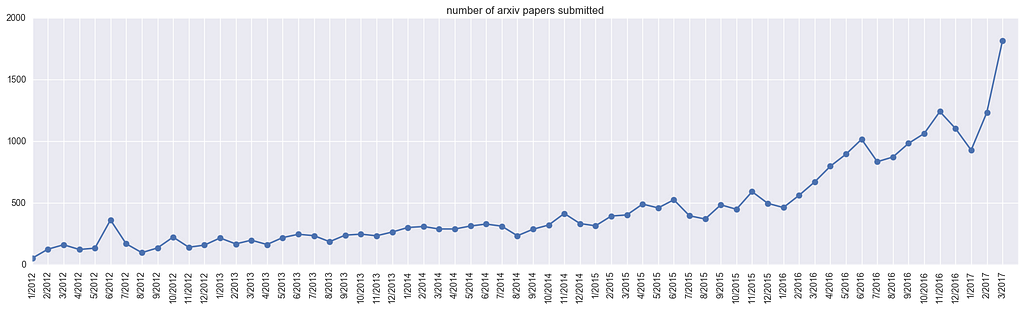
Let’s first look at the total number of submitted papers across the arxiv-sanity categories (cs.AI,cs.LG,cs.CV,cs.CL,cs.NE,stat.ML), over time. We get the following:
Yes, March of 2017 saw almost 2,000 submissions in these areas. The peaks are likely due to conference deadlines (e.g. NIPS/ICML). Note that this is not directly a statement about the size of the area itself, since not everyone submits their paper to arxiv, and the fraction of people who do likely changes over time. But the point remains — that’s a lot of papers to be aware of, skim, or (gasp) read.
This total number of papers will serve as the denominator. We can now look at what fraction of papers contain certain keywords of interest.
Deep Learning Frameworks
To warm up let’s look at the Deep Learning frameworks that are in use. To compute this, we record the fraction of papers that mention the framework somewhere in the full text (anywhere — including bibliography etc). For papers uploaded on March 2017, we get the following:
% of papers 	 framework 	 has been around for (months)
------------------------------------------------------------
    9.1          tensorflow       16
    7.1               caffe       37
    4.6              theano       54
    3.3               torch       37
    2.5               keras       19
    1.7          matconvnet       26
    1.2             lasagne       23
    0.5             chainer       16
    0.3               mxnet       17
    0.3                cntk       13
    0.2             pytorch       1
    0.1      deeplearning4j       14
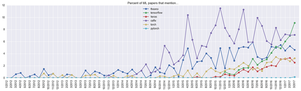
That is, 10% of all papers submitted in March 2017 mention TensorFlow. Of course, not every paper declares the framework used, but if we assume that papers declare the framework with some fixed random probability independent of the framework, then it looks like about 40% of the community is currently using TensorFlow (or a bit more, if you count Keras with the TF backend). And here is the plot of how some of the more popular frameworks evolved over time:
We can see that Theano has been around for a while but its growth has somewhat stalled. Caffe shot up quickly in 2014, but was overtaken by the TensorFlow singularity in the last few months. Torch (and the very recent PyTorch) are also climbing up, slow and steady. It will be fun to watch this develop in the next few months — my own guess is that Caffe/Theano will go on a slow decline and TF growth will become a bit slower due to PyTorch.
ConvNet Models
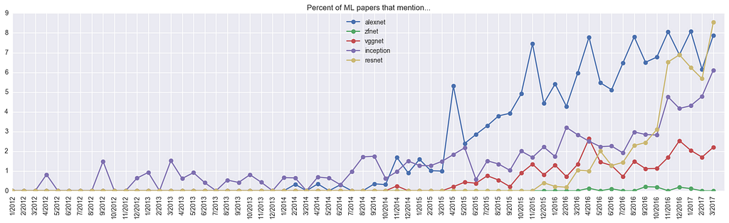
For fun, how about if we look at common ConvNet models? Here, we can clearly see a huge spike up for ResNets, to the point that they occur in 9% of all papers last March:
Also, who was talking about “inception” before the InceptionNet? Curious.
Optimization algorithms
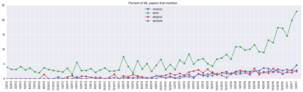
In terms of optimization algorithms, it looks like Adam is on a roll, found in about 23% of papers! The actual fraction of use is hard to estimate; it’s likely higher than 23% because some papers don’t declare the optimization algorithm, and a good chunk of papers might not even be optimizing any neural network at all. It’s then likely lower by about 5%, which is the “background activity” of “Adam”, likely a collision with author names, as the Adam optimization algorithm was only released on Dec 2014.
Researchers
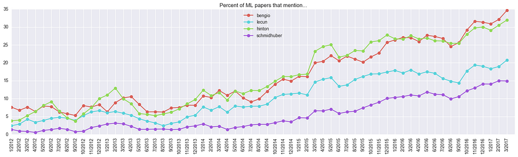
I was also curious to plot the mentions of some of the most senior PIs in Deep Learning (this gives something similar to citation count, but 1) it is more robust across population of papers with a “0/1” count, and 2) it is normalized by the total size of the pie):
A few things to note: “bengio” is mentioned in 35% of all submissions, but there are two Bengios: Samy and Yoshua, who add up on this plot. In particular, Geoff Hinton is mentioned in more than 30% of all new papers! That seems like a lot.
Hot or Not Keywords
Finally, instead of manually going by categories of keywords, let’s actively look at the keywords that are “hot” (or not).
Top hot keywords
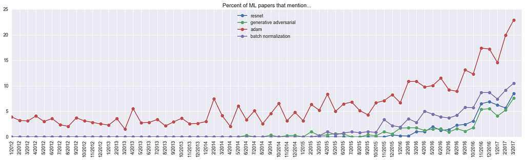
There are many ways to define this, but for this experiment I look at each unigram or bigram in all the papers and record the ratio of its max use last year compared to its max use up to last year. The papers that excel at this metric are those that one year ago were niche, but this year appear with a much higher relative frequency. The top list (slightly edited out some duplicates) comes out as follows:
For example, ResNet’s ratio of 8.17 is because until 1 year ago it appeared in up to only 1.044% of all submissions (in Mar 2016), but last last month (Mar 2017) it appeared in 8.53% of submissions, so 8.53 / 1.044 ~= 8.17. So there you have it — the core innovations that became all the rage over the last year are 1) ResNets, 2) GANs, 3) Adam, 4) BatchNorm. Use more of these to fit in with your friends. In terms of research interests, we see 1) style transfer, 2) deep RL, 3) Neural Machine Translation (“nmt”), and perhaps 4) image generation. And architecturally, it is hot to use 1) Fully Convolutional Nets (FCN), 2) LSTMs/GRUs, 3) Siamese nets, and 4) Encoder decoder nets.
Top not hot
How about the reverse? What has seen many fewer submissions over the last year than has historically had a higher “mind share”? Here are a few:
I’m not sure what “fractal” is referring to, but more generally it looks like bayesian nonparametrics are under attack.
Conclusion
Now is the time to submit paper on Fully Convolutional Encoder Decoder BatchNorm ResNet GAN applied to Style Transfer, optimized with Adam. Hey, that doesn’t even sound too far-fetched.
Are you exploring AI? If so, well then just try to at least socialize with others exploring AI once in a while 😉 We’re connecting people like you in the AI community together to discuss advancements, share opportunities, sketch ideas, and connect. This event is just social, so no laptop is required, but you will need one for the next workshop we’re planning 🙂 Bring an inquisitive mind and let’s see you there!
Bring your own laptop, we’ll be diving into some artificial intelligence. Also, we’ll be looking at setting up some actual code with some of the libraries out there which we’ll build upon for with future meetups. We’ll be introducing a hello-world equivalent using the scikit framework for this session.
Whether you’re a beginner or an expert, all that matters is your interest in the subject, the rest will work itself out
When we offered CS231n (Deep Learning class) at Stanford, we intentionally designed the programming assignments to include explicit calculations involved in backpropagation on the lowest level. The students had to implement the forward and the backward pass of each layer in raw numpy. Inevitably, some students complained on the class message boards:
“Why do we have to write the backward pass when frameworks in the real world, such as TensorFlow, compute them for you automatically?”
This is seemingly a perfectly sensible appeal – if you’re never going to write backward passes once the class is over, why practice writing them? Are we just torturing the students for our own amusement? Some easy answers could make arguments along the lines of “it’s worth knowing what’s under the hood as an intellectual curiosity”, or perhaps “you might want to improve on the core algorithm later”, but there is a much stronger and practical argument, which I wanted to devote a whole post to:
> The problem with Backpropagation is that it is a leaky abstraction.
In other words, it is easy to fall into the trap of abstracting away the learning process — believing that you can simply stack arbitrary layers together and backprop will “magically make them work” on your data. So lets look at a few explicit examples where this is not the case in quite unintuitive ways.
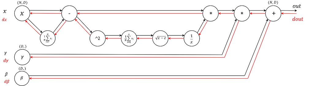
Some eye candy: a computational graph of a Batch Norm layer with a forward pass (black) and backward pass (red). (borrowed from this post)
Vanishing gradients on sigmoids
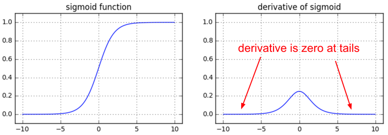
We’re starting off easy here. At one point it was fashionable to use sigmoid (or tanh) non-linearities in the fully connected layers. The tricky part people might not realize until they think about the backward pass is that if you are sloppy with the weight initialization or data preprocessing these non-linearities can “saturate” and entirely stop learning — your training loss will be flat and refuse to go down. For example, a fully connected layer with sigmoid non-linearity computes (using raw numpy):
z = 1/(1 + np.exp(-np.dot(W, x))) # forward pass
dx = np.dot(W.T, z*(1-z)) # backward pass: local gradient for x
dW = np.outer(z*(1-z), x) # backward pass: local gradient for W
If your weight matrix W is initialized too large, the output of the matrix multiply could have a very large range (e.g. numbers between -400 and 400), which will make all outputs in the vector z almost binary: either 1 or 0. But if that is the case, z*(1-z), which is local gradient of the sigmoid non-linearity, will in both cases become zero (“vanish”), making the gradient for both x and W be zero. The rest of the backward pass will come out all zero from this point on due to multiplication in the chain rule.
Another non-obvious fun fact about sigmoid is that its local gradient (z*(1-z)) achieves a maximum at 0.25, when z = 0.5. That means that every time the gradient signal flows through a sigmoid gate, its magnitude always diminishes by one quarter (or more). If you’re using basic SGD, this would make the lower layers of a network train much slower than the higher ones.
TLDR: if you’re using sigmoids or tanh non-linearities in your network and you understand backpropagation you should always be nervous about making sure that the initialization doesn’t cause them to be fully saturated. See a longer explanation in this CS231n lecture video.
Dying ReLUs
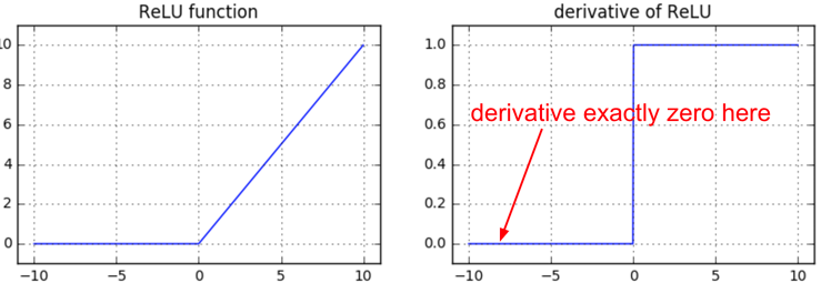
Another fun non-linearity is the ReLU, which thresholds neurons at zero from below. The forward and backward pass for a fully connected layer that uses ReLU would at the core include:
z = np.maximum(0, np.dot(W, x)) # forward pass
dW = np.outer(z > 0, x) # backward pass: local gradient for W
If you stare at this for a while you’ll see that if a neuron gets clamped to zero in the forward pass (i.e. z=0, it doesn’t “fire”), then its weights will get zero gradient. This can lead to what is called the “dead ReLU” problem, where if a ReLU neuron is unfortunately initialized such that it never fires, or if a neuron’s weights ever get knocked off with a large update during training into this regime, then this neuron will remain permanently dead. It’s like permanent, irrecoverable brain damage. Sometimes you can forward the entire training set through a trained network and find that a large fraction (e.g. 40%) of your neurons were zero the entire time.
TLDR: If you understand backpropagation and your network has ReLUs, you’re always nervous about dead ReLUs. These are neurons that never turn on for any example in your entire training set, and will remain permanently dead. Neurons can also die during training, usually as a symptom of aggressive learning rates. See a longer explanation in CS231n lecture video.
Exploding gradients in RNNs
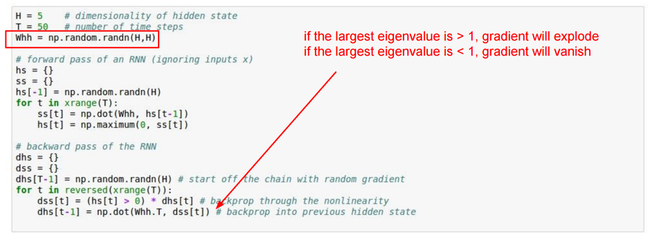
Vanilla RNNs feature another good example of unintuitive effects of backpropagation. I’ll copy paste a slide from CS231n that has a simplified RNN that does not take any input x, and only computes the recurrence on the hidden state (equivalently, the input x could always be zero):
This RNN is unrolled for T time steps. When you stare at what the backward pass is doing, you’ll see that the gradient signal going backwards in time through all the hidden states is always being multiplied by the same matrix (the recurrence matrix Whh), interspersed with non-linearity backprop.
What happens when you take one number a and start multiplying it by some other number b (i.e. a*b*b*b*b*b*b…)? This sequence either goes to zero if |b| < 1, or explodes to infinity when |b|>1. The same thing happens in the backward pass of an RNN, except b is a matrix and not just a number, so we have to reason about its largest eigenvalue instead.
TLDR: If you understand backpropagation and you’re using RNNs you are nervous about having to do gradient clipping, or you prefer to use an LSTM. See a longer explanation in this CS231n lecture video.
Spotted in the Wild: DQN Clipping
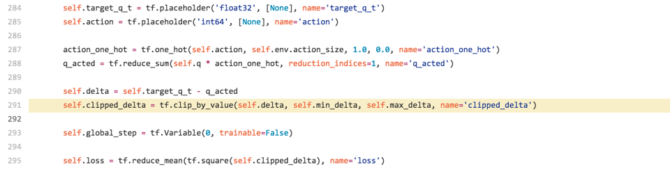
Lets look at one more — the one that actually inspired this post. Yesterday I was browsing for a Deep Q Learning implementation in TensorFlow (to see how others deal with computing the numpy equivalent of Q[:, a], where a is an integer vector — turns out this trivial operation is not supported in TF). Anyway, I searched “dqn tensorflow”, clicked the first link, and found the core code. Here is an excerpt:
If you’re familiar with DQN, you can see that there is the target_q_t, which is just [reward * gamma argmax_a Q(s’,a)], and then there is q_acted, which is Q(s,a) of the action that was taken. The authors here subtract the two into variable delta, which they then want to minimize on line 295 with the L2 loss with tf.reduce_mean(tf.square()). So far so good.
The problem is on line 291. The authors are trying to be robust to outliers, so if the delta is too large, they clip it with tf.clip_by_value. This is well-intentioned and looks sensible from the perspective of the forward pass, but it introduces a major bug if you think about the backward pass.
The clip_by_value function has a local gradient of zero outside of the range min_delta to max_delta, so whenever the delta is above min/max_delta, the gradient becomes exactly zero during backprop. The authors are clipping the raw Q delta, when they are likely trying to clip the gradient for added robustness. In that case the correct thing to do is to use the Huber loss in place of tf.square:
It’s a bit gross in TensorFlow because all we want to do is clip the gradient if it is above a threshold, but since we can’t meddle with the gradients directly we have to do it in this round-about way of defining the Huber loss. In Torch this would be much more simple.
I submitted an issue on the DQN repo and this was promptly fixed.
In conclusion
Backpropagation is a leaky abstraction; it is a credit assignment scheme with non-trivial consequences. If you try to ignore how it works under the hood because “TensorFlow automagically makes my networks learn”, you will not be ready to wrestle with the dangers it presents, and you will be much less effective at building and debugging neural networks.
The good news is that backpropagation is not that difficult to understand, if presented properly. I have relatively strong feelings on this topic because it seems to me that 95% of backpropagation materials out there present it all wrong, filling pages with mechanical math. Instead, I would recommend the CS231n lecture on backprop which emphasizes intuition (yay for shameless self-advertising). And if you can spare the time, as a bonus, work through the CS231n assignments, which get you to write backprop manually and help you solidify your understanding.
That’s it for now! I hope you’ll be much more suspicious of backpropagation going forward and think carefully through what the backward pass is doing. Also, I’m aware that this post has (unintentionally!) turned into several CS231n ads. Apologies for that 🙂
My favorite among these was the session with Patrick (video), which I found to be rich with interesting points and mental models. In what follows I will try to do a brain dump of some of these ideas in my own words.
On organizational structure (~20min mark)
I found Patrick’s slight resentment of new organizational structure ideas refreshing and amusing. We hear a lot about disruption, thinking from first principles, being contrarian, etc. Patrick was trying to make the point that the mean organizational structure of a company that we’ve converged on (e.g. hierarchies etc.), and the way things are done is actually quite alright. That in fact we know a lot about how to organize groups of people towards a common goal, and that one must resist the temptation to be too clever with it. He also conceded that a lot of things have changed over the last several years (especially with respect to technology), but made the point that human psychology has in comparison stayed nearly constant, which means we can more confidently draw on past knowledge in these areas.
This part was quite amusing because I felt like Patrick was being contrarian by defending the standard.
On hiring (~28 min mark)
Several interesting points — first, it has become meaningless to regurgitate the fact that hiring is very important. What that actually means when you want to translate it to a statement with actual bits of information, Patrick argues, is to rephrase it as “you have to be very very persistent” in recruiting the best people, and willing to to do it very slowly over time (e.g. they took 6 months to hire 2 employees early on).
Another interesting analogy was in thinking of good people as airship carriers. Your job during hiring is to find them and steer them towards a direction, as opposed to thinking about it the other way around, where you try to find people aligned with your direction first and then build them up over time. The argument is in favor of the former order of precedence.
The last point that resonated with me strongly was the realization that it is incorrect to think about hiring on an individual basis. When you’re hiring a person you’re in fact hiring an entire cone of people in expectation, because good people in an area attract more good people like them, dramatically reducing the barrier for another similar hire.
Company communication
I also really liked the idea that as the company grows more, the communication channels should tend toward writing more than talking. The comparison to the printing press was interesting, and the notion that what made writing so powerful was not only the dissemination, but also the concreteness and rigidity of written text. The fact that writing encourages the full serialization a concept, much more than a speech. The idea that you can point to paragraph 2, sentence 5 and say “no, that’s wrong”.
The misc
The entire conversation was peppered with interesting mental models for thinking about different facets of companies: The idea that an optimal 1-year plan can be very distinct from the optimal 5-year plan. The idea of Stripe as a blob in a philosophical space, and that different people within the organization are in different angles/distances with respect to its center of mass, and have to be actively pulled towards it. The 3 jobs of a CEO. etcetc.
Misc misc
There were also several other interesting insights from the other guests, which I will dump here in an unsorted form.
The SurveyMonkey back story was fun to hear about — a great example of an organically rapidly growing company with huge profit margins. Also, an example of a company that may seem not too exciting until you think about it more. Selina also made the interesting observation that some people have preferences towards particular stages of the company, and that some might not scale, or not be willing to scale, up.
Nirav described a very nice example of doing things that don’t scale with the early days of Nextdoor. They attracted only 170 neighborhoods in their first year, by hand. Nirav also mentioned an interesting concept of a “treadmill company” – a metaphor for a company where you can’t easily step back and enjoy the view — it requires constant struggle and active involvement. Finally, in terms of extracting value from customers without explicitly charging them Nirav mentioned two modes of operation: the demand fulfillment model (e.g. Google) and demand generation model (e.g. Facebook).
Shishir brought up an interesting idea called the “tombstone test”, as a way of determining how to spend your time. In short, if you can’t imagine something being on your tombstone then it is not worth working on. Hm!
That’s it! The insights I like the most are the ones that point out mental models that distill a situation to something that preserves most of its core dynamics, but is easier to think about. This distillation process cleans an idea, strips it from the irrelevant and preserves the core nugget of insight. The last few weeks were quite rich!