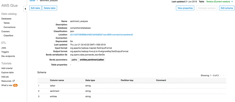
We’ve heard from customers that scaling TensorFlow training jobs to multiple nodes and GPUs successfully is hard. TensorFlow has distributed training built-in, but it can be difficult to use. Recently, we made optimizations to TensorFlow and Horovod to help AWS customers scale TensorFlow training jobs to multiple nodes and GPUs. With these improvements, any AWS customer can use an AWS Deep Learning AMI to train ResNet-50 on ImageNet in just under 15 minutes.
To achieve this, 32 Amazon EC2 instances, each with 8 GPUs, a total 256 GPUs, were harnessed with TensorFlow. All of the required software and tools for this solution ship with the latest Deep Learning AMIs (DLAMIs), so you can try it out yourself. You can train faster, implement your models faster, and get results faster than ever before. This blog post describes our results and shows you how to try out this easier and faster way to run distributed training with TensorFlow.

Figure A. ResNet-50 ImageNet model training with the latest optimized TensorFlow with Horovod on a Deep Learning AMI takes 15 minutes on 256 GPUs.
Training a large model takes time, and the larger and more complex the model is, the longer the training is going to take. If your business requirement is to generate updated models on a regular basis, any training that takes too long means missed opportunities. A typical response is to throw more processing power at the problem, but for deep learning, the communications overhead during training has made this approach infeasible or profoundly expensive. This communications overhead results in a loss of efficiency, significantly reducing your throughput and increasing your time to train. It can also be complex to set up the required infrastructure and reach required levels of accuracy. TensorFlow supports distributed training natively, but in our experiments, we obtained better results (in both speed and accuracy) when we incorporated Horovod.
Horovod is a popular choice for distributed training. Take, for example, the recent use of Horovod with 27,000 GPUs to analyze climate change. Orchestrating this number of GPUs would be impossible without proper tooling. With Horovod, using software optimizations and Amazon EC2 p3 instances, we were able to limit the efficiency loss to 15 percent, resulting in a time-to-train under 15 minutes.
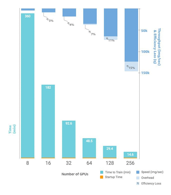
Figure B. Time to train vs number of GPUs vs images per second, communication overhead, and efficiency. Startup time is a consistent 1.5 minutes regardless of cluster size.
All of the tools you need to try this out are shipped on the latest DLAMI. This includes example scripts for training ResNet-50 with ImageNet. If you’re ready to roll up your sleeves now and try it out, continue reading. The rest of this blog post shows you how you can use EC2 p3 instances, TensorFlow, and Horovod to train ResNet-50 on ImageNet in under 15 minutes.
How to train ResNet/ImageNet in under 15 minutes with TensorFlow
I first tried out Horovod with TensorFlow on the Deep Learning AMI (DLAMI). I was asked to write a tutorial on using Horovod to train ImageNet on an eight-GPU EC2 instance. I wondered what on earth was Uber thinking when they named their distributed training framework “Horovod”, and I wondered how much time was this going to take? Training ImageNet takes forever, and Horovod sounds like some villain from the Harry Potter universe. It’s not. It was created by Alexander Sergeev at Uber. He named it after Russian & eastern European folk dance where a large group of dancers perform synchronized moves in a circle. It turned out to be a fun way to learn how to dance with Horovod using up to 8 GPUs in one DLAMI.
That was a couple of months ago, and now I’m going to show you what the the TensorFlow team here at Amazon AI has been up to. They’ve been fine-tuning Horovod with TensorFlow, and the implementation on the DLAMI is much faster. More importantly, you can run upwards of 256 GPUs in one training run to train ResNet-50 on ImageNet in under 15 minutes!
The first time I ran Horovod on a DLAMI was on a p3.16xlarge EC2 instance. This beast of an instance has eight Tesla V100 GPUs. Horovod uses all of the instance’s GPUs to turn a training time that could take more than a day to a training time that could be finished in a few hours. I used the latest DLAMI so I wouldn’t have to install and configure CUDA, TensorFlow, or Horovod. I could activate the environment with one command, and then execute the training script with another one liner.
Setup was easy. Training was relatively fast – only slightly sub-linear scaling from one to eight GPUs. It finished in eight hours and the accuracy was acceptable: 75.4% for top-1 and 92.6% for top-5. Based on this result, I wrote the Tensorflow-Horovod tutorial for the DLAMI .
Next, I asked myself how fast I can train ResNet-50 on several p3 instances. I knew that scaling efficiency will never be 100% and that, in total, people will end up paying more. However, if your team was waiting for a model to train for a day, they would think training in 15 minutes was worth the savings on developers’ productivity. This is especially true because the efficiency loss of the faster training, as our experiments demonstrate, is minimal.
We recently benchmarked running 256 GPUs with great accuracy and an even faster completion time. Don’t you want to try that out yourself? Does your dance card even have 256 slots? Keep reading and I’ll walk you through how we can make this happen.
With the latest updates to the DLAMI and its TensorFlow-Horovod environment you could train ResNet-50 on all of ImageNet for about a 20% cost reduction compared to its release. In this blog post we’ll demonstrate how fast things can go and scale, and save your wallet for future dances with Horovod. Are you ready?
The original TensorFlow-Horovod tutorial shows you a single node implementation. You spin up one instance and use all of its GPUs. This time I’ll show you how you can spin up several nodes, link them up with a Horovod configuration, and then run the training. We’ll run some benchmarks, so you can estimate your time for completion and see what your efficiency loss is for each new node. With this info you can estimate your costs, and then apply this pattern to other models that you want to train.
Part 1: Spin up a bunch of DLAMIs
Now is a good time to plan out your moves with a quick questionnaire:
- Do you need to get a copy of ImageNet?
- If yes:
- Spin up one DLAMI for now. Downloading and prepping the dataset can take several hours, and you don’t want several instances sitting around, racking up your bill while you wait. You can add more DLAMIs later. If you want to be clever, you can run the download and prep steps faster with a big DLAMI CPU instance, then transfer it to your DLAMI GPU instances for training when it is ready. You could also divide up the dataset and prep the dataset across multiple machines.
- If no: go to 2.
- Do you have an ImageNet dataset already downloaded to your AWS environment – on Amazon S3, a shared volume, or on an instance?
- If yes:
- Later in this blog I’ll give you some bash functions that can help you distribute the dataset to each node.
- If no:
- Only spin up one instance for now. Get it ready there, then spin up the rest and distribute the dataset using one of the functions I just mentioned.
- Is your ImageNet dataset already preprocessed for training with TensorFlow?
- If yes:
- You’re going to be able to do everything in this blog post pretty quickly, even train ImageNet entirely in about an hour-and-a-half with just four instances.
- If no:
- Follow these detailed instructions in DLAMI’s docs on how to prepare the ImageNet dataset.
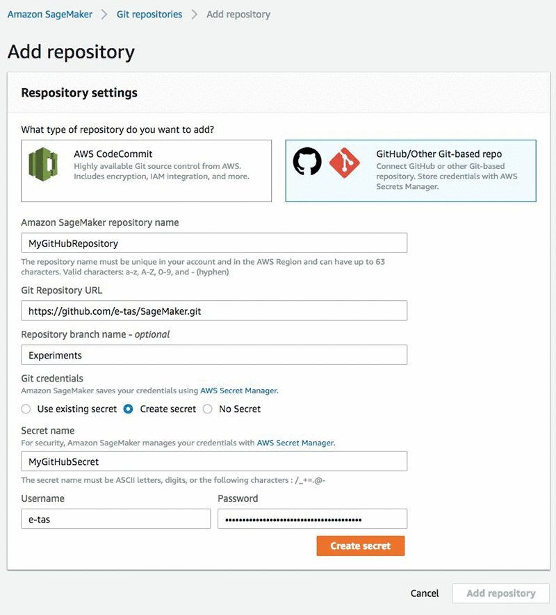
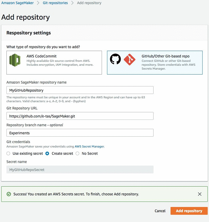
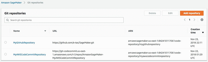
Now let’s spin up one or more DLAMIs. There are several ways you can do this, but I’m going to use the Amazon EC2 console. If you already know how to use AWS Cloud Formation templates or the AWS CLI, you can use those tools as well. The goal here is to launch some number of identical DLAMIs that each have more than one GPU. For this next step, I’m going to launch four p3.16xlarge DLAMIs all in the same Region and security zone (VPC). This step is important. You can’t just link up random instances you have that are launched in different Regions or security zones without impacting performance.
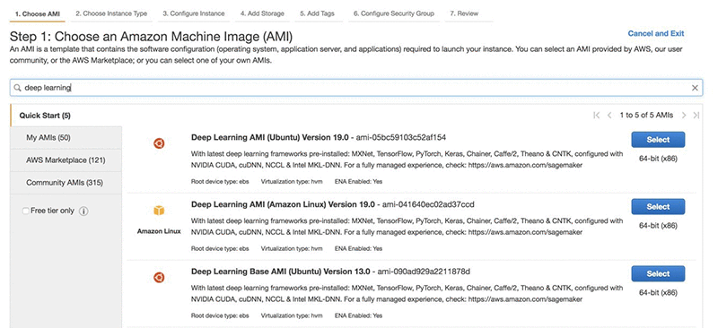
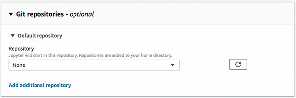
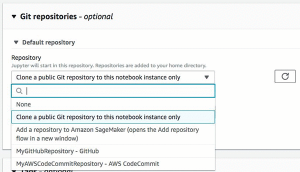
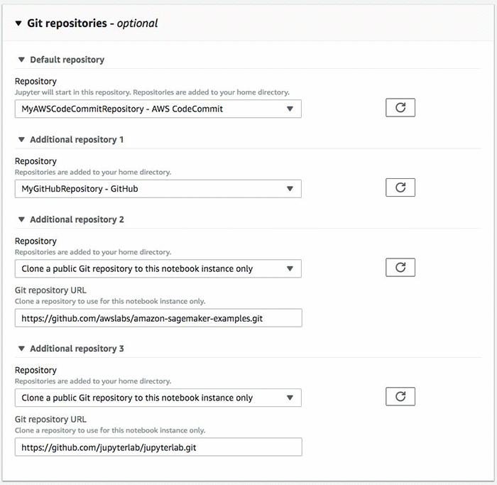
On the EC2 console you can search for an AMI by name. Search for “deep learning” and you will find Deep Learning AMI (Ubuntu). Choose the Select button.
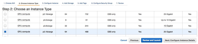
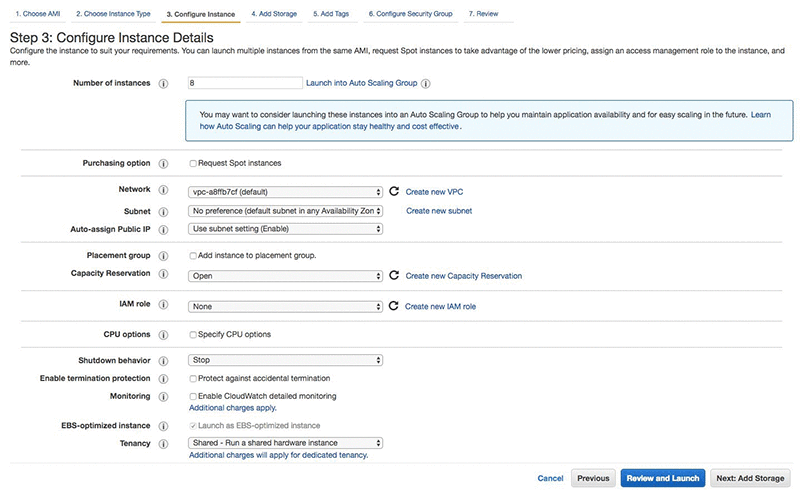
After you select the Deep Learning AMI (Ubuntu) you can choose the instance type. Since we want to use the faster instance to achieve the fastest training, choose the p3dn.24xl instance type. If this is not available yet in your Region, choose the p3.16xlarge instead. The more GPUs you have on the same system, the faster your training will be. Now choose Next: Configure Instance Details. You have the option of launching multiple identical instances. Choose up to 32 instances to achieve 256 GPU training. For the purposes of this example, however, I’ll use 4 instances, with a total of 32 GPUs.
Next, choose your instance details. You should choose an instance with at least 200 GB of fast storage. I’m choosing a Provisioned IOPS SSD with 10,000 IOPS to get the best performance.

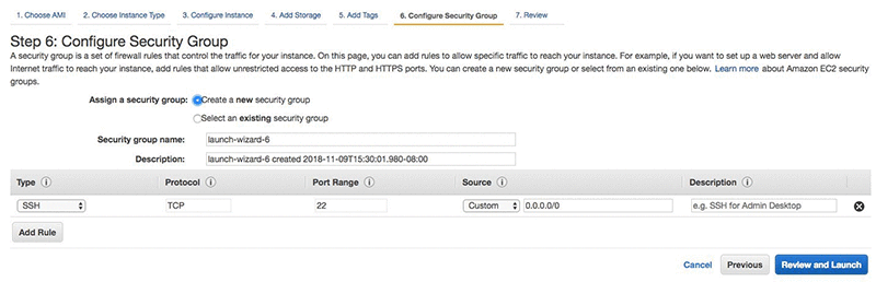
You can just skip through the tags screen and continue to Configure Security Group.

On the security group settings page, you can create a new group, or use an existing one. Next, review your choices, make corrections as needed, and then choose Review and Launch.
Your screen should look much like the following screenshot. Important things to note are in the storage section: size, volume type, and IOPS. Choose Launch.
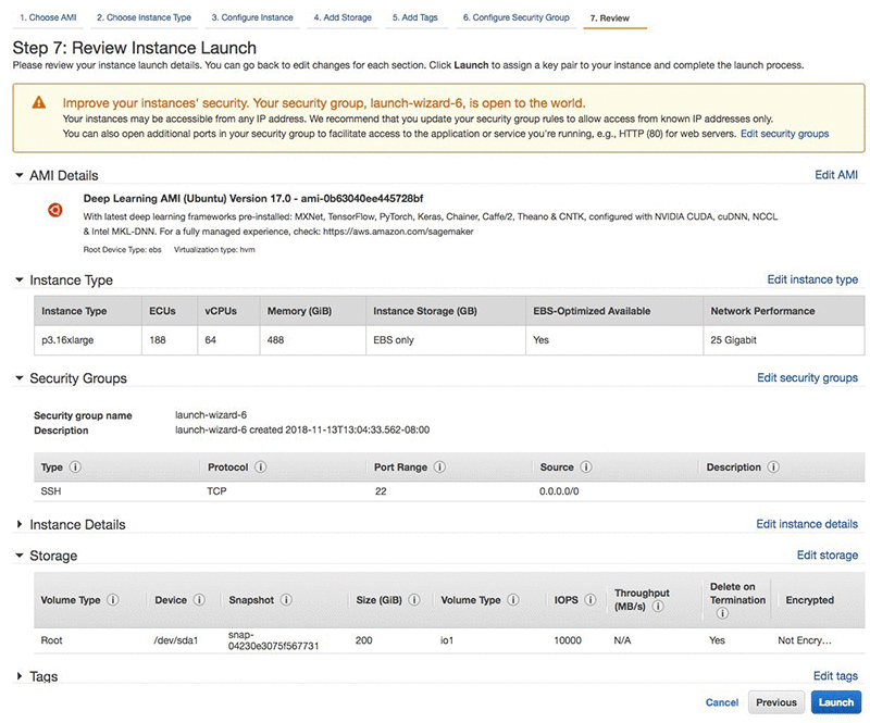
After choosing Launch, you’ll select a key pair. Use existing keys or create new ones. Make note of where you put your keys and what you named them because you will need this information later.

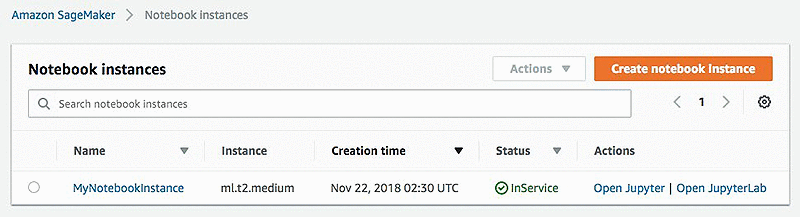
If you get a green box, choose View Instances to review the list of the freshly launch DLAMIs.

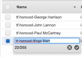
It takes a couple of minutes to launch the instances, so now is a good time to name them.
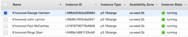
Select one of your DLAMIs. Rename it in the console so you don’t forget which one is which. If you have 8 nodes, you could call them Snow White and the Seven Dwarves (Doc, Dopey, Bashful, Grumpy, Sneezy, Sleepy, and Happy). I only launched four, so I called them John Lennon, Paul McCartney, George Harrison, and Ringo Starr. I chose John Lennon to be the leader. Some people like to call the leader the master, but I prefer “leader.” There’s a leader and members.
Part 2: Prep the dataset
Step 1. Download a copy of ImageNet to each new cluster of DLAMIs.
For the fastest performance you will want each instance in your cluster to have a local copy of the dataset. The raw dataset needs to be preprocessed by a TensorFlow utility before you train with it. Otherwise, training will take longer, and you won’t see the accuracy levels that are reported in most benchmarks. If you don’t have ImageNet handy, you’ll need to download it. Even if you do have a copy, you will need this data to be inside your cluster’s Region and security zone, and it will need that previously mentioned preprocessing. So, if you have a preprocessed copy ready on Amazon S3 or elsewhere, great, copy it to your leader, then you can skip ahead to Part 3.
Download ImageNet to one of your instances now, or if you already have it somewhere, copy it to an instance now, and then read ahead. This way you’ll know what is coming, and in Part 3 you can try out distributed training with a synthetic dataset while you wait.
Step 2. Prep the ImageNet files for training.
You need to run a preparation step prior to training. This preprocesses all of the images, so that they’re consistent and optimized for training speed. Without running this step you can’t hope to achieve comparable speed or accuracy. Your costs will certainly be higher. Note that after you run this step once, you don’t have to do it again for subsequent training runs. You might want to keep this volume around and connect it to future DLAMIs and tests or benchmarking runs.
Follow these detailed instructions in DLAMI’s docs on how to prepare the ImageNet dataset.
I must admit that I already had my preprocessed copy of ImageNet sitting around, so that’s why I said the setup and training was so easy. Now that you’ve done the preprocessing, you’ll want to keep yours too. You can stop any one of your instances without terminating it, then bring the instance back along with the data sometime in the future! You could also save the preprocessed dataset to S3 to archive it for later use.
Part 3: training with synthetic data
While you wait for ImageNet to download, you can try the setup with synthetic data. This will assure that your members can talk to each other, TensorFlow with Horovod is working in this multi-node mode, and that eventually you can switch to training with the ImageNet dataset.
Before you move on to the next step, review the overall settings, making sure each node is running, is the same instance type and is in the same Availability Zone.
In the console, choose the leader, choose the Actions button, and then choose Connect. The next page provides instructions for connecting. If you created a new key, you will need to adjust its security settings with chmod 400 key.pem. These instructions are in the Connect prompt. However, one important variation in how you connect with ssh is that you want your leader to be able to access your members. You do this by adding your key and customizing your ssh login to be slightly different than what is suggested by the Connect prompt. Run the following commands from your local terminal and the directory where you downloaded your key. Be sure to swap out “key.pem” with the filename of the key and “PUBLIC_IP_ADDRESS_OF_THE_LEADER” before running it.
ssh-add -K key.pem
ssh -A ubuntu@PUBLIC_IP_ADDRESS_OF_THE_LEADER
Once connected, activate the tensorflow_p36 environment.
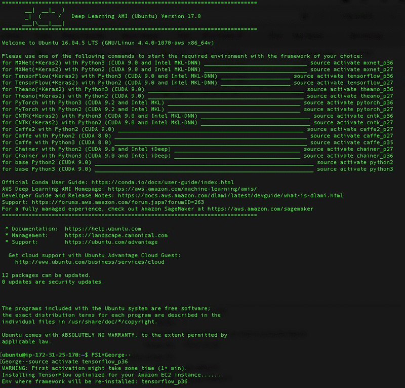
In this example, I’m launching John Lennon now. After I have logged in, I’ll start the TensorFlow environment. You will likely see TensorFlow being optimized for the instance type, so this first activation may take a moment.
source activate tensorflow_p36
After activating the environment we must let Horovod know about the rest of the band. This is achieved by adding each member’s info to a hosts file. Change directories to where the training scripts reside.
cd ~/examples/horovod/tensorflow
Use vim to edit a file in the leader’s home directory.
Select one of the members in the EC2 console, and the description page opens. Find the Private IPs field and copy the IP address and paste it in a text file. Copy each member’s private IP address on a new line. Then, next to each IP address add a space and then the text slots=8. This represents how many GPUs each instance has. The p3.16xlarge instances have 8 GPUs, so if you chose a different instance type, you would provide the actual number of GPUs for each instance. For the leader you can use localhost. It should look similar to the following:
172.100.1.200 slots=8
172.200.8.99 slots=8
172.48.3.124 slots=8
localhost slots=8
Save the file and exit back to the leader’s terminal.
Now your leader knows how to reach each member. This is all going to happen on the private network interfaces. Next, use a short bash function to help send commands to each member. Run this command in your leader’s terminal session:
function runclust(){ while read -u 10 host; do host=${host%% slots*}; ssh -o "StrictHostKeyChecking no" $host ""$2""; done 10<$1; };
First tell the other members to not do “StrickHostKeyChecking” as this may cause training to hang.
runclust hosts "echo "StrictHostKeyChecking no" >> ~/.ssh/config"
Now it is time to try out the training with synthetic data. The script deep-learning-models/models/resnet/tensorflow/dlami_scripts/train_synthetic.sh will default to 8 GPUs, but you can provide it the number of GPUs you want to run. Run the script, passing 4 as a parameter for the 4 GPUs we’re using for this run.
After some warning messages you will see the following output that verifies Horovod is using 4 GPUs.
PY3.6.5 |Anaconda custom (64-bit)| (default, Apr 29 2018, 16:14:56)
[GCC 7.2.0]TF1.11.0
Horovod size: 4
Then after some other warnings you see the start of a table and some data points. You break out of the training if you don’t want to watch for 1,000 batches. Here I stop it at 400 since I can see that the training is averaging about 3,000 images per second.
   Step Epoch  Speed  Loss   FinLoss LR
     0   0.0   105.6  6.794  7.708 6.40000
     1   0.0   311.7  0.000  4.315 6.38721
   100   0.1  3010.2  0.000 34.446 5.18400
   200   0.2  3013.6  0.000 13.077 4.09600
   300   0.2  3012.8  0.000  6.196 3.13600
   400   0.3  3012.5  0.000  3.551 2.30401
Let’s try 8 GPUs.
I stopped at 200 this time once I saw that the speed was a little less than double: 5,874 vs 3,012.
   Step Epoch  Speed  Loss   FinLoss LR
    0    0.0   200.5  6.804   7.718 6.40000
    1    0.0   564.2  0.000   6.878 6.38721
  100    0.2  5871.7  0.000  60.158 5.18400
  200    0.3  5874.3  0.000  22.838 4.09600
Now you’re ready to test multi-node training. Try out the full 32 GPUs.
Your output will be similar. You will see the Horovod size at 32, and you will see roughly 4 times the speed. With this experimentation completed, you will have tested your leader and its ability to communicate with the members. If you run into any issues, check the troubleshooting section in the Horovod tutorials docs.
Part 4: Train ResNet-50 on ImageNet
After you’re satisfied watching the synthetic data training step and you’ve prepared the ImageNet dataset, you’re ready to copy the prepared dataset to all of the members.
If you still only have the dataset on your leader, use this copyclust function to copy data over to other members. Run this command in your leader’s terminal session:
function copyclust(){ while read -u 10 host; do host=${host%% slots*}; rsync -azv "$2" $host:"$3"; done 10<$1; };
Now you can use copyclust to copy the dataset folder. The first param is the hosts file, the second is the dataset folder on your leader, and the third is the target directory on each member:
copyclust hosts ~/imagenet_data ~/imagenet_data
Or, if you have the files sitting in an Amazon S3 bucket, use the runclust function to download the files to each member directly.
runclust hosts "tmux new-session -d "export AWS_ACCESS_KEY_ID=YOUR_ACCESS_KEY && export AWS_SECRET_ACCESS_KEY=YOUR_SECRET && aws s3 sync s3://your-imagenet-bucket ~/imagenet_data/ && aws s3 sync s3://your-imagenet-validation-bucket ~/imagenet_data/""
There’s something to be said here about using tmux or screen or some tools to let you disconnect and resume sessions. Using tools that let you manage multiple nodes at once is a great timesaver. But, I’m going to gloss over this part because it goes beyond the scope of this blog. You have many options: wait around for each step and manage each instance separately or use some power tools.
After the copying is completed, you’re ready to start training. Run the script, passing 32 as a parameter for the 32 GPUs we’re using for this run. Use tmux or a similar tool if you’re concerned about disconnecting and terminating your session, thereby aborting the training run.
The following output is what you see when running the training on ImageNet with 32 GPUs. 32 GPUs will take 90-110 minutes.
   Step Epoch  Speed  Loss   FinLoss LR
     0   0.0   440.6  6.935  7.850 0.00100
     1   0.0  2215.4  6.923  7.837 0.00305
    50   0.3 19347.5  6.515  7.425 0.10353
   100   0.6 18631.7  6.275  7.173 0.20606
   150   1.0 19742.0  6.043  6.922 0.30860
   200   1.3 19790.7  5.730  6.586 0.41113
   250   1.6 20309.4  5.631  6.458 0.51366
   300   1.9 19943.9  5.233  6.027 0.61619
   350   2.2 19329.8  5.101  5.864 0.71872
   400   2.6 19605.4  4.787  5.519 0.82126
   450   2.9 20025.5  5.020  5.725 0.92379
   500   3.2 19526.8  4.702  5.383 1.02632
   550   3.5 18102.1  4.632  5.294 1.12885
   600   3.8 19450.3  4.377  5.023 1.23138
   650   4.2 19845.1  3.738  4.372 1.33392
   700   4.5 18838.6  3.862  4.488 1.43645
   750   4.8 19572.7  3.435  4.059 1.53898
   800   5.1 20697.7  3.388  4.015 1.64151
   850   5.4 19651.1  3.141  3.774 1.74405
   900   5.8 20012.3  3.231  3.878 1.84658
   950   6.1 19261.0  3.039  3.699 1.94911
  1000   6.4 18248.2  2.969  3.645 2.05164
  1050   6.7 18730.4  2.731  3.429 2.15417
  ...
   13750  87.9 19398.8  0.676  1.082 0.00217
 13800  88.2 19827.5  0.662  1.067 0.00156
 13850  88.6 19986.7  0.591  0.997 0.00104
 13900  88.9 19595.1  0.598  1.003 0.00064
 13950  89.2 19721.8  0.633  1.039 0.00033
 14000  89.5 19567.8  0.567  0.973 0.00012
 14050  89.8 20902.4  0.803  1.209 0.00002
Finished in 6004.354426383972
This run completed! It follows up with an evaluation run. It will run on the leader as it will run quickly enough without having to distribute the job to the other members. The following is the output of the evaluation run.
Horovod size: 32
Evaluating
Validation dataset size: 50000
 step  epoch  top1    top5     loss   checkpoint_time(UTC)
14075   90.0  75.716   92.91    0.97  2018-11-14 08:38:28
If you’re curious what this output looks like with 256 GPUs, you can check it out in the following output block.
  Step Epoch  Speed    Loss   FinLoss LR
  1550  79.3 142660.9  1.002  1.470 0.04059
  1600  81.8 143302.2  0.981  1.439 0.02190
  1650  84.4 144808.2  0.740  1.192 0.00987
  1700  87.0 144790.6  0.909  1.359 0.00313
  1750  89.5 143499.8  0.844  1.293 0.00026
Finished in 860.5105031204224

Finished evaluation
1759   90.0  75.086   92.47    0.99  2018-11-20 07:18:18
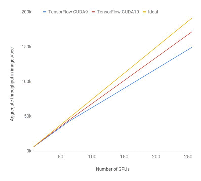
You can see that the speed in images/sec is over 140k. The following chart shows the latest benchmarks with CUDA10 using 256 GPUs which reaches speeds of 171k! This improves efficiency to 90%. Look for this to ship on the DLAMI after TensorFlow releases an official binary for CUDA 10. The following chart shows the Performance of ResNet-50 training using CUDA 10. Overhead is reduced compared to CUDA 9.
Conclusion
Now that you’ve tried four nodes, do you want to try more? How about 16 or 32 nodes? Or how about 2? You can scale up or down and see how that impacts performance. Compare epoch training times and estimate your overall cost for completion.
Note: if you use the “more like this” feature in the Amazon EC2 console, be prepared to adjust all of the settings, most notably the storage. “More like this” doesn’t include storage, so make sure you update that to have at least 200 GB.
You might want to also try a different dataset and see how fast you can train it using the latest instance types and optimized TensorFlow environments on the DLAMI.
Stay tuned for our next blog where we apply the latest improvements in scalable training on a cluster of DLAMIs.
Appendix
Troubleshooting
The following command might help you get past errors that come up when you experiment with Horovod.
- If the training crashes, mpirun may fail to clean up all the Python processes on each machine. In that case, before you start the next job kill the Python processes on all machines as follows:
- runclust hosts “pkill -9 python”
- If the process finishes abruptly without error, try deleting your log folder.
- If other unexplained issues pop up, check your disk space. If you’re out of space, try removing the logs folder since that is full of checkpoints and data. You can also increase the size of the volumes for each member.
- As a last resort you can also try rebooting.
# kill python
runclust hosts "pkill -9 python"
# delete log folder
runclust hosts "rm -rf ~/imagenet_resnet/"
# check disk space
runclust hosts "df /"
# reboot
runclust hosts "sudo reboot"
About the Author
 Aaron Markham is a programmer writer for MXNet and AWS Deep Learning AMI. He has a degree in winemaking and a passion for new technology which he shares by writing and teaching. Aside from talking about deep learning tech, he teaches computer skills to the homeless in Santa Cruz and web programming to prisoners at San Quentin. When not working or teaching, you can find him on the slopes snowboarding or hiking.
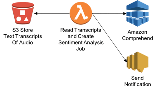

 Deenadayaalan Thirugnanasambandam is a Senior Cloud Architect in the Professional Services team in Australia.
 Piyush Patel is a big data consultant with AWS.
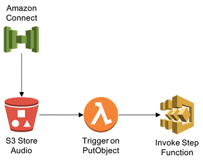
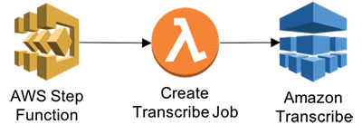
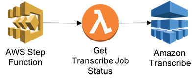
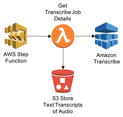
 Paul Zhao is a Sr. Product Manager at AWS Machine Learning. He manages the Amazon Transcribe service. Outside of work, Paul is a motorcycle enthusiast and avid woodworker.
 Revanth Anireddy is a professional services consultant with AWS.
 Loc Trinh is a Solutions Architect for AWS Database and Analytics services. In his spare time, he captures data from his eating and fitness habits and uses analytical modeling to determine why he is still out of shape.


 Huibin Shen is an applied scientist in Amazon AI. He works in the part of the team that launched the Automatic Model Tuning feature in Amazon SageMaker.
 Fan Li is a Product Manager of Amazon SageMaker. He used to be a big fan of ballroom dance but now loves whatever his 8-year-old son likes.
 Miroslav Miladinovic is a Software Development Manager at Amazon SageMaker.


 Raja Mani is a Solution Architect supporting AWS partners. He is interested in Serverless development, DevOps, Containers, Big Data and Machine Learning. He is helping AWS partners to architect the enterprise-grade Amazon Web Services Solutions for their customers.
 Luis Pineda is a Partner Solutions Architect at Amazon Web Services based in Chicago. He works with our partners and customers to solve business problems using AWS. Outside of work, Luis enjoys being outdoors, running, cycling and soccer.


 Yong Seong Lee is a Cloud Support Engineer for AWS Big Data Services. He is interested in every technology related to Big Data/Data Analysis/Machine Learning and helping customers who have difficulties in using AWS services. His motto is “Enjoy life, be curious and have maximum experience.”


 Cameron Peron is Sr. Developer Marketing Manager for Artificial Intelligence at Amazon Web Services.
 Sumit Thakur is a Senior Product Manager for AWS Machine Learning Platforms where he loves working on products that make it easy for customers to get started with machine learning on cloud. He is product manager for Amazon SageMaker and AWS Deep Learning AMI. In his spare time, he likes connecting with nature and watching sci-fi TV series.
 Erkan Tas is a Senior Product Manager for Amazon SageMaker. He is on a mission to make Artificial Intelligence easy, accessible, and scalable through AWS platforms. He is also a sailor, science and nature admirer, Go and Stratocaster player.
 Ragav Venkatesan is a Research Scientist with AWS AI Labs. He has an MS in Electrical Engineering and a PhD in Computer Science from Arizona State University. His current area of research includes Neural Network compression and Computer Vision algorithms for Amazon SageMaker. Outside of work, Ragav is a session bassist and producer at Thaalam Studios.
 Saksham Saini did his BS in Computer Engineering from University of Illinois at Urbana-Champaign. He is currently working on building highly optimized and scalable algorithms for Amazon SageMaker. Outside work, he enjoys reading, music and traveling.
 Satyaki Chakraborty is an MS student at Carnegie Mellon University studying computer vision. He contributed to Amazon SageMaker Semantic Segmentation during his summer internship.
 Xiong Zhou is an Applied Scientist with AWS AI Labs. He has a PhD in Electrical and Electronics Engineering from University of Houston. His current research focus involves developing domain adaptation and active learning algorithms. He is also working on building computer vision algorithms for Amazon SageMaker.
 Luka Krajcar is a Software Development Engineer on the AWS AI Algorithms team. He received his M.S. in Computer Science at the Faculty of Electrical Engineering and Computing at the University of Zagreb. Outside of work, Luka enjoys reading fiction, running, and video gaming.
 Hang Zhang is an Applied Scientist with Amazon AI. He has a PhD from Rutgers University. He is currently working with the GluonCV team.
 Yoni Friedman is a Sr. Technical Product Manager in the AWS Artificial Intelligence team where he leads product management for Amazon Translate. He spends his free time reading, running, playing ball, and doing other stuff his two toddlers ask him to.