Category: Global
What’s Up, Doc?: AI Startup Gives Patients the Power
AI, when applied to healthcare, holds the promise of better medical predictions and faster medicinal improvements. To do so, it needs data on which to train. But healthcare data is sensitive and private, creating a dead end.
Or not. Walter De Brouwer, CEO of Silicon Valley startup doc.ai, joined AI Podcast host Noah Kravitz to discuss how his medical research-based platform makes the application of deep learning to healthcare possible.
Many consumers worry about the outcome of putting their data in the cloud, where it risks being pirated. And larger institutions like hospitals that have an abundance of healthcare data are reticent to share it because it could reveal other sensitive business information.
Doc.ai first collects everything it needs from the device and user input. It takes into account data from Apple Health, blood tests, urine analysis, and any other medical information uploaded by the client.
The platform has eight prediction models, which exist locally on the client’s device. Each module has a specific focus, from the general medical record, to urine sampling, to phenomics.
These models transform the data into tensors — what De Brouwer calls “a big pile of numbers.” They’re then uploaded to the cloud with no risk of being pirated, because without the model that produced them, they’re like “GPS coordinates on planet Jupiter – you can’t do anything with it.”
From there, doc.ai can use these tensors to improve its deep learning algorithms and improve medical predictions.
Doc.ai also provides a platform to run medical trials. Clients and doctors can create their own, or take part in the three that De Brouwer has already organized. The first is organized in collaboration with advisors from Harvard Medical School, and focuses on allergy triggers. Another, studying the various combinations of the 26 medicines designed to treat epilepsy, was designed alongside Stanford specialists.
De Brouwer is no stranger to entrepreneurship. He’s the cofounder of several AI-based companies, including Inui Health, which performs urine analysis using machine learning and mobile phones, and XY.ai, a spinoff of Harvard Medical School that uses AI for large-scale digital twin technology.
De Brouwer is certain that doc.ai has found the ideal approach for improving healthcare knowledge. “This is Darwinism,” he says. “First you collect, then you predict, and then you change the bad things and amplify the good things. These three steps are basically the evolution algorithm of the planet.”
To learn more about doc.ai, visit their website here. Or visit their blog for weekly stories, as well as Github commands and Jupyter notebooks.
Help Make the AI Podcast Better
Have a few minutes to spare? Fill out this short listener survey. Your answers will help us make a better podcast.
How to Tune in to the AI Podcast
Get the AI Podcast through iTunes, Castbox, DoggCatcher, Overcast, PlayerFM, Podbay, PodBean, Pocket Casts, PodCruncher, PodKicker, Stitcher, Soundcloud and TuneIn. Your favorite not listed here? Email us at aipodcast [at] nvidia [dot] com.
The post What’s Up, Doc?: AI Startup Gives Patients the Power appeared first on The Official NVIDIA Blog.
Parallelizing across multiple CPU/GPUs to speed up deep learning inference at the edge
AWS customers often choose to run machine learning (ML) inferences at the edge to minimize latency. In many of these situations, ML predictions must be run on a large number of inputs independently. For example, running an object detection model on each frame of a video. In these cases, parallelizing ML inferences across all available CPU/GPUs on the edge device offers the potential to reduce the overall inference time.
Recently, my team recognized a need for this optimization while helping a customer to build an industrial anomaly detection system. In this use case, a set of cameras took and uploaded images of passing machines (about 3,000 images per machine). The customer needed each image fed into a deep learning-based object detection model they had deployed to an edge device at their site. The edge hardware at each site had two GPUs and several CPUs. Initially, we implemented a long-running Lambda function (more on this later in the post) deployed to an AWS IoT Greengrass core. This configuration would process each image sequentially on the edge device.
However, this configuration runs deep learning inference on a single CPU and a single GPU core of the edge device. To reduce inference time, we considered how to take advantage of the available hardware’s full capacity. After some research, I found documentation (for various deep learning frameworks) on many ways to distribute training among multiple CPU/GPUs (such as TensorFlow, MXNet, and PyTorch). However, I did not find material on how to parallelize inference on a given host.
In this post, I will show you several ways to parallelize inference, providing example code snippets and performance benchmark results.
This post focuses exclusively on data parallelism. This means dividing the list of input data into equal parts and having each CPU/GPU core process one such part. This approach differs from model parallelism, which entails splitting an ML model into different parts and loading each part into a different processor. Data parallelism is much more common and practical due to its simplicity.
What’s hard about parallelizing ML inference on a single machine?
If you are a software engineer familiar with writing multi-threaded code, you might read the preceding and wonder: What’s challenging about parallelizing ML inferences on a single machine? To better understand this, let’s quickly review the process of doing a single ML inference end-to-end, assuming that your device has at least one GPU:

Here are some considerations when you think about optimizing inference performance on a machine with multiple CPU/GPUs:
- Heavy initialization: In the diagrammed process, Step 1 (loading the neural net), often takes a significant amount of time—loading times of a few hundred milliseconds or multiple seconds are typical. Given the timing, I recommend that you perform initialization once per process/thread and reuse the process/thread for running inference.
- Either CPU or GPU can be the bottleneck: Step 2 (data transformation), and Step 4 (forward pass on the neural net) are the two most computationally intensive steps. Depending on the complexity of the code and the available hardware, you might find that one use case utilizes 100% of your CPU core while underutilizing your GPU, while another use case does the opposite.
- Explicitly assigning GPUs to process/threads: When using deep learning frameworks for inference on a GPU, your code must specify the GPU ID onto which you want the model to load. For example, if you have two GPUs on a machine and two processes to run inferences in parallel, your code should explicitly assign one process GPU-0 and the other GPU-1.
- Ordering outputs: Do you need the output ordered before being consumed by downstream processing? When you parallelize different inputs for simultaneous processing by different threads, First-In-First-Out guarantees no longer apply. For example, in a real-time object tracking system, the tracking algorithm must process the prediction of the previous video frame before processing the prediction of the next frame. In such cases, you must implement additional indexing and reordering after the parallelized inference takes place. In other use cases, out-of-order results might not be an issue.
Summary of parallelization approaches
In this post, I show you three options for parallelizing inference on a single machine. Here’s a quick glimpse of their pros and cons.
| Option | Pros | Cons | Recommended? |
| 1A: Using multiple long-lived AWS Lambda functions in AWS IoT Greengrass |
|
|
Yes |
| 1B: Using on-demand Lambda functions in AWS IoT Greengrass |
|
|
No |
| 2: Using Python multiprocessing |
|
|
Yes |
Parallelization option 1: Using multiple Lambda containers in AWS IoT Greengrass
AWS IoT Greengrass is a great option for running ML inference at the edge. It enables devices to run Lambda functions locally on the edge device and respond to events, even during disrupted cloud connectivity. When the device reconnects to the internet, the AWS IoT Greengrass software can seamlessly synchronize any data you want to upload to the cloud for further analytics and durable storage. As a result, you enjoy the benefits of both running ML inferences locally at the edge (that is, lower latency, network bandwidth savings, and potentially lower cost) and scalable analytics and storage capabilities of the cloud for the data that must persist.
AWS IoT Greengrass also includes a feature to help you manage machine learning resources while deploying ML inference at the edge. Use this feature to specify where on Amazon S3 you want the ML model parameter files stored. AWS IoT Greengrass downloads and extracts the files to a designated location on the edge device during deployment. This feature simplifies ML model updates. When you have a new ML model, point the ML resource to the new artifact’s S3 location and trigger a new deployment of the Greengrass group. Any changes to the source ML artifact on S3 automatically redeploy to the edge device.
If you run your inference code with AWS IoT Greengrass, you can also parallelize inferences by running multiple inference Lambda function instances in parallel. You can do this in two ways in AWS IoT Greengrass: Using multiple, long-lived Lambda functions or on-demand Lambda.
Option 1A: Using multiple long-lived Greengrass Lambda functions (recommended)
A long-lived (or pinned) Greengrass Lambda function resembles a daemon process. Unlike AWS Lambda functions in the cloud, the long-lived Greengrass Lambda function creates a single container for each function. The same container queues and processes requests to that Lambda function, one by one.
Using a long-lived Greengrass Lambda function for ML minimizes the impact of the initialization latency. Within a long-lived Greengrass Lambda function, you load the ML model once during initialization. Any subsequent request reuses the same container without having to load the ML model again.
In this paradigm, you can parallelize inferences by defining multiple, long-lived Greengrass Lambda functions running the same source code. Configuring two long-lived Greengrass Lambda functions on one AWS IoT Greengrass core results in two long-running containers, each with the ML model initialized and ready to run inferences concurrently. Some pros and cons of this approach:
Pros of using long-lived Greengrass Lambda functions
- Keep the inference code simple. You don’t need to change your single-threaded inference code.
- You can assign different GPUs to each of the Greengrass Lambda functions by specifying different environment variables for them.
- You can rely on AWS IoT Greengrass to maintain the desired number of concurrent inference containers. Even if one container crashes due to some unhandled exception, the AWS IoT Greengrass core software launches a new, replacement container.
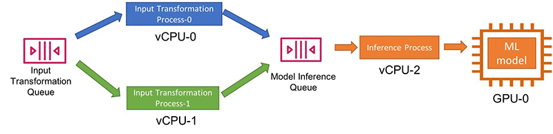
- You can also rely on Greengrass constructs to decouple the CPU-intensive input transformation computation and the GPU-intensive forward-pass portion into separate Lambda functions, further optimizing resource use. For example, assume that the data transformation code is the bottleneck in the inference, and there are four CPU cores and two GPU cores on the machine. In that case, you can have four long-running Lambda functions for data transformation (one for each CPU core) and pass the results into two long-running Lambda functions (one for each GPU core).
Cons of using long-lived Greengrass Lambda functions
- Each long-lived Lambda function processes inputs one-by-one. As a result, you should implement load balancing logic to split the inputs into distinct topics to which separate Lambda functions subscribe.For example, if you have two concurrent inference Lambda functions, you can write a preprocessing Lambda function splitting the inputs in half and assigning each half on a separate IoT topic in AWS IoT Greengrass. The following diagram illustrates this workflow:

- As of May 2019, AWS IoT Greengrass limits the number of Lambda containers that can run concurrently to 20. All Lambda functions on the AWS IoT Greengrass core device share this hard limit, including on-demand containers. If you have other Lambda functions performing processing tasks on the same device, this limit might prevent you from running multiple Lambda instances for each inference task.
- This approach requires hardcoding configurations for an AWS IoT Greengrass deployment, such as the number of long-running inference Lambda functions, the GPU IDs to which they are assigned, and the corresponding input subscriptions. You must know the hardware specs of each device that you plan to use before deployment. If you operate a heterogeneous fleet of devices with different numbers of cores, you must provide specific AWS IoT Greengrass configurations mapping to the CPU/GPU resources of each device model.
Option 1B: Using on-demand Greengrass Lambda functions (not recommended)
On-demand Greengrass Lambda functions work similarly to AWS Lambda functions in the cloud. When multiple requests come in, AWS IoT Greengrass can dynamically spin up multiple containers (or sandboxes). Any container can process any invocation, and they can run in parallel.
When no tasks are left to execute, the containers (or sandboxes) can persist, and future invocations can reuse them. Alternatively, they can be terminated to make room for other Lambda function executions. You cannot control the number of containers that get spun up nor how many of them persist. A heuristic internal to AWS IoT Greengrass determines the number of containers based on the queue size. In short, using the on-demand Lambda configuration, AWS IoT Greengrass dynamically scales the number of containers that execute your code, based on traffic.
This configuration fits data processing use cases with low initialization overhead. However, there are several disadvantages when using the on-demand configuration for deep learning inference code:
- “Cold Start” latency: As mentioned previously, deep learning models take a while to load into memory. While AWS IoT Greengrass dynamically spins up and destroys containers, incoming requests might require new container creation and incur initialization latency. Such delays could negate the performance gains from parallelization.
- Lack of control on the number of concurrent containers: Controlling the number of concurrent inference Lambda function executions helps optimize resource use. For example, imagine you have two GPUs, and each forward pass process of the ML model uses 100% of the GPU. In that scenario, two concurrent Greengrass Lambda containers would represent the ideal use of your resources. Creating more than two containers would only result in more context-switching and queueing for CPU/GPU resources. The on-demand Lambda configuration doesn’t permit you to control the number of concurrent executions.
- Difficulty in coordination between concurrent Lambda containers: Usually, the on-demand model assumes that each concurrent Lambda container instance is independent and configured in the same way. However, when you use multiple GPUs, you must explicitly assign each Lambda container to use a different GPU. These GPU assignments require some coordination among containers, as AWS IoT Greengrass dynamically spins them up and destroys them.
Parallelization option 2: Using Python multiprocessing (recommended)
The previously discussed option 1A might not be appropriate for those who:
- Prefer not to use AWS IoT Greengrass
- Need to run many Lambda functions, and having multiple instances of each would exceed the concurrent container limit of Greengrass
- Want to flexibly determine the level of parallelization at runtime, based on available hardware resources
An alternative for those users would be to change your inference code to take advantage of multiple cores. I discuss this option in the following section, focusing on Python, given the language’s unmatched popularity in the ML and data science space.
Python multiprocessing
Programming languages like Java or C++ let you use multiple threads to take advantage of multiple CPU cores. Unfortunately, Python’s global interpreter lock (GIL) prevents you from parallelizing inference in this way. However, you can use Python’s multiprocessing module to achieve parallelism by running ML inference concurrently on multiple CPU and GPUs. Supported in both Python 2 and Python 3, the Python multiprocessing module lets you spawn multiple processes that run concurrently on multiple processor cores.
Using process pools to parallelize inference
The Python multiprocessing module offers process pools. Using process pools, you can spawn multiple long-lived processes and load a copy of the ML model in each process during initialization. You can then use the pool.Map () function to submit a list of inputs to be processed by the pool. See the following code snippet example:
You can read the rest of the inference script in the parallelize-ml-inference GitHub repo. This multiprocessing code can run inside a single Greengrass Lambda function as well.
An example benchmark using Python multiprocessing process pools
How much does this parallelization improve performance? Using the cited multiprocessing pool code, I ran an object detection MXNet model on a p3.8xlarge instance (which has four NVIDIA Tesla V100 GPUs) to see how different process pool sizes affect the total time needed to process 3000 images. The object detection model I used (a model trained with the Amazon SageMaker built-in SSD algorithm) produced the following results:

A few observations about this experiment:
- For this combination of input transformation code, inference code, dataset, and hardware spec, total inference time improved from 153 seconds using a single process to about 40 seconds by parallelizing the task across CPU/GPUS in multiple processes (almost 1/4 of the time).
- In this experiment, the bottleneck appears to be the CPU and input transformation. The GPU is under-utilized both from a memory and processing perspective. See the following snapshot of GPU utilization when the script run with two worker processes. (The p3.8xlarge instance has four GPUs. Therefore, you can see two of them idle when I ran the script with only two processes).
As the utilization metric above shows, one loaded ML model used about 1 GB of memory from the 16 GB available on each GPU. So in this case, you can actually load more than one model per GPU, with each performing inference independently on a separate set of inputs. The script above supports more processes than the number of GPUs by assigning each process a looping list of GPU IDs.
So, when I tested with eight processes, the script assigns one GPU ID from the list [0, 1, 2, 3, 0, 1, 2, 3] to load the ML model to each process. Keep in mind that the two ML models loaded on the same GPU are independent copies of the same model. Each model can perform inferences independently on separate inputs. If I try to load more model copies than the GPU memory can accommodate, an out-of-memory error occurs.
On the CPU side, because a p3.8xlarge instance included 32 vCPUs and I ran fewer than 32 processes, each process could run on a dedicated vCPU. You can confirm CPU utilization during the experiment by running htop. See the following illustration for how this worked on the processors:

Using outputs from htop and nvidia-smi commands, I could confirm that the bottleneck in this particular experiment was the input transformation step on the CPUs. (The CPUs in use were 100% utilized while the GPUs were not).
We can gain additional insight into the impact of parallelization by measuring the duration of processing a single input. The following graph compares the p50 (median) timings for the two processing steps, as recorded by the worker processes. As the graph shows, the GPU inference time increases only slightly as I packed multiple ML models onto each GPU. However, input transformation time per image continues to climb up as more worker processes were used (thus vCPUs), implying some contention that require further code optimization.
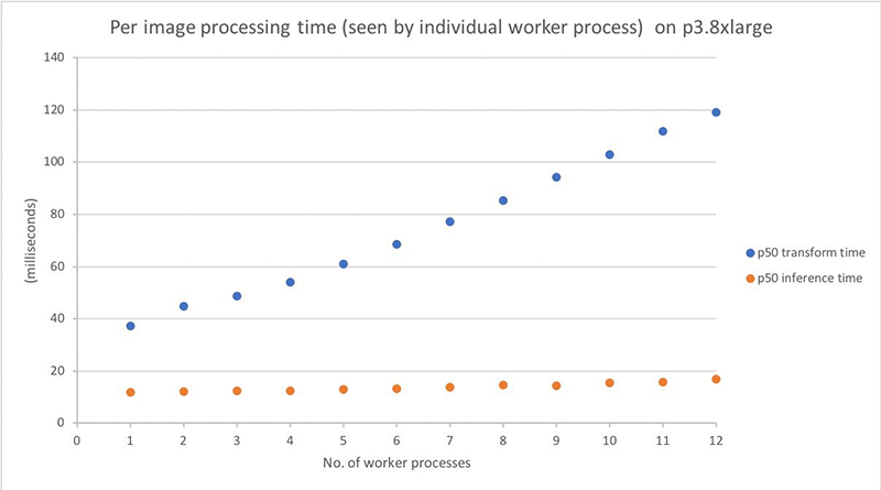
The processing time graph might make you wonder why the per-image processing time increases with the number of processes, while the total process time decreases. Remember: per-image timing graph above is measured from each worker process as they run in parallel. The total processing time roughly equals the following:

General learning and considerations
In addition to the described experiment, I also tried to run similar tests with different frameworks, models, and hardware. Here are some takeaways from those experiments:
Not all deep learning frameworks support multiprocessing inference equally. The process pool script runs smoothly with an MXNet model. By contrast, the Caffe2 framework crashes when I try to load a second model to a second process. Others have reported similar issues on GitHub for Caffe2. I found little or no documentation on multithreading/multiprocessing inference support from the major frameworks. So, you should test this yourself with your framework of choice.
Different hardware and inference code require different multiprocessing strategy. In my experiment, the model is relatively small compared to the GPU capacity. I could load multiple ML models to run inference simultaneously on a single GPU.
By contrast, less powerful devices and more heavyweight models might restrict you to one model per GPU, with a single inference task using 100% of the GPU. If the input transformation remains slow compared to the model inference, and if you have more CPUs than GPUs, you can also decouple them and use a different number of processes for each step using Python multiprocessing queues.
In the provided benchmarking code, I used process pools and pool.map() for code simplicity. In contrast, a publisher-consumer model with queues between processes offers a lot more flexibility (if some added code complexity):
There are other ways to improve inference performance. Many other available approaches also offer improved inference performance. For example, you can use Amazon SageMaker Neo to convert your trained model to an efficient format optimized for the underlying hardware, achieving faster performance while lowering memory footprint.
Another approach to explore is batching. In the cited test, I perform object detection inference for one image at a time. Batching multiple images for simultaneous processing offers to speed up total inference through matrix math efficiencies implemented by the underlying libraries and hardware optimizations. However, if you are trying to obtain results in real time, batching might not always be an option.
Try enabling NVIDIA Multi-Process Service (MPS). If you use an NVIDIA GPU device, you can enable Multi-Process Service (MPS) on each GPU. MPS offers an alternative GPU configuration to support running multiple ML models, submitted simultaneously from multiple CPU processes, on a single GPU. You can use either of the AWS IoT Greengrass or pure Python approach with MPS enabled or disabled.
I completed the example benchmark results described earlier on the p3.8xlarge instance without enabling MPS. I found the GPU on the p3.8xlarge supported running multiple independent ML models out of the box. When I tested the same setup with MPS turned on, the results showed an almost-negligible performance improvement (that is, by 0.2 milliseconds per image). However, I recommend that you try enabling MPS for your specific hardware and use case. You might find that it significantly improves performance.
Conclusion
In this post, I discussed two approaches for parallelizing inference on a single device at the edge across multiple CPU/GPUs:
- Run multiple Lambda containers (long-lived or on-demand) inside the AWS IoT Greengrass core
- Use Python multiprocessing
The former offers code simplicity, while the latter can run within or without Greengrass and provides the maximum flexibility. I also showed an example benchmark test highlighting the performance improvement you can obtain using multiple CPU/GPUs for inference. If your inference hardware is underutilized, give these options a try!
To start using AWS IoT Greengrass, click here. To start exporing SageMaker Neo, click here. You can find the code used in this post in the parallelize-ml-inference GitHub repo.
About the author
 Angela Wang is an R&D Engineer on the AWS Solutions Architecture team based in New York city. She helps AWS customers build out innovative ideas by rapid prototyping using the AWS platform. Outside of work, she loves reading, climbing, backcountry skiing and traveling.
Turbo, An Improved Rainbow Colormap for Visualization
False color maps show up in many applications in computer vision and machine learning, from visualizing depth images to more abstract uses, such as image differencing. Colorizing images helps the human visual system pick out detail, estimate quantitative values, and notice patterns in data in a more intuitive fashion. However, the choice of color map can have a significant impact on a given task. For example, interpretation of “rainbow maps” have been linked to lower accuracy in mission critical applications, such as medical imaging. Still, in many applications, “rainbow maps” are preferred since they show more detail (at the expense of accuracy) and allow for quicker visual assessment.
 |
| Left: Disparity image displayed as greyscale. Right: The commonly used Jet rainbow map being used to create a false color image. |
One of the most commonly used color mapping algorithms in computer vision applications is Jet, which is high contrast, making it useful for accentuating even weakly distinguished image features. However, if you look at the color map gradient, one can see distinct “bands” of color, most notably in the cyan and yellow regions. This causes sharp transitions when the map is applied to images, which are misleading when the underlying data is actually smoothly varying. Because the rate at which the color changes ‘perceptually’ is not constant, Jet is not perceptually uniform. These effects are even more pronounced for users that are color blind, to the point of making the map ambiguous:
 |
| The above image with simulated Protanopia |
Today there are many modern alternatives that are uniform and color blind accessible, such as Viridis or Inferno from matplotlib. While these linear lightness maps solve many important issues with Jet, their constraints may make them suboptimal for day to day tasks where the requirements are not as stringent.
 |
 |
| Viridis | Inferno |
Today we are happy to introduce Turbo, a new colormap that has the desirable properties of Jet while also addressing some of its shortcomings, such as false detail, banding and color blindness ambiguity. Turbo was hand-crafted and fine-tuned to be effective for a variety of visualization tasks. You can find the color map data and usage instructions for Python here and C/C++ here, as well as a polynomial approximation here.
Development
To create the Turbo color map, we created a simple interface that allowed us to interactively adjust the sRGB curves using a 7-knot cubic spline, while comparing the result on a selection of sample images as well as other well known color maps.
 |
| Screenshot of the interface used to create and tune Turbo. |
This approach provides control while keeping the curve C2 continuous. The resulting color map is not “perceptually linear” in the quantitative sense, but it is more smooth than Jet, without introducing false detail.
 |
| Turbo |
 |
| Jet |
Comparison with Common Color Maps
Viridis is a linear color map that is generally recommended when false color is needed because it is pleasant to the eye and it fixes most issues with Jet. Inferno has the same linear properties of Viridis, but is higher contrast, making it better for picking out detail. However, some feel that it can be harsh on the eyes. While this isn’t a concern for publishing, it does affect people’s choice when they must spend extended periods examining visualizations.
 |
 |
| Turbo | Jet |
 |
 |
| Viridis | Inferno |
Because of rapid color and lightness changes, Jet accentuates detail in the background that is less apparent with Viridis and even Inferno. Depending on the data, some detail may be lost entirely to the naked eye. The background in the following images is barely distinguishable with Inferno (which is already punchier than Viridis), but clear with Turbo.
 |
 |
| Inferno | Turbo |
Turbo mimics the lightness profile of Jet, going from low to high back down to low, without banding. As such, its lightness slope is generally double that of Viridis, allowing subtle changes to be more easily seen. This is a valuable feature, since it greatly enhances detail when color can be used to disambiguate the low and high ends.
 |
 |
| Turbo | Jet |
 |
 |
| Viridis | Inferno |
| Lightness plots generated by converting the sRGB values to CIECAM02-UCS and displaying the lightness value (J) in greyscale. The black line traces the lightness value from the low end of the color map (left) to the high end (right). |
The Viridis and Inferno plots are linear, with Inferno exhibiting a higher slope and over a broader range. Jet’s plot is erratic and peaky, and banding can be seen clearly even in the grayscale image. Turbo has a similar asymmetric profile to Jet with the lows darker than the highs.This is intentional, to make cases where low values appear next to high values more distinct. The curvature in the lower region is also different from the higher region, due to the way blues are perceived in comparison to reds.
Although this low-high-low curve increases detail, it comes at the cost of lightness ambiguity. When rendered in grayscale, the coloration will be ambiguous, since some of the lower values will look identical to higher values. Consequently, Turbo is inappropriate for grayscale printing and for people with the rare case of achromatopsia.
Semantic Layers
When examining disparity maps, it is often desirable to compare values on different sides of the image at a glance. This task is much easier when values can be mentally mapped to a distinct semantic color, such as red or blue. Thus, having more colors helps the estimation ease and accuracy.
 |
 |
| Turbo | Jet |
 |
 |
| Viridis | Inferno |
With Jet and Turbo, it’s easy to see which objects on the left of the frame are at the same depth as objects on the right, even though there is a visual gap in the middle. For example, you can easily spot which sphere on the left is at the same depth as the ring on the right. This is much harder to determine using Viridis or Inferno, which have far fewer distinct colors. Compared to Jet, Turbo is also much more smooth and has no “false layers” due to banding. You can see this improvement more clearly if the incoming values are quantized:
 |
| Left: Quantized Turbo colormap. Up to 33 quantized colors remain distinguishable and smooth in both lightness and hue change. Right: Quantized Jet color map. Many neighboring colors appear the same; Yellow and Cyan colors appear brighter than the rest. |
Quick Judging
When doing a quick comparison of two images, it’s much easier to judge the differences in color than in lightness (because our attention system prioritizes hue). For example, imagine we have an output image from a depth estimation algorithm beside the ground truth. With Turbo it’s easy to discern whether or not the two are in agreement and which regions may disagree.
 |
 |
| “Output” Viridis | “Ground Truth” Viridis |
 |
 |
| “Output” Turbo | “Ground Truth” Turbo |
In addition, it is easy to estimate quantitative values, since they map to distinguishable and memorable colors.

Diverging Map Use Cases
Although the Turbo color map was designed for sequential use (i.e., values [0-1]), it can be used as a diverging colormap as well, as is needed in difference images, for example. When used this way, zero is green, negative values are shades of blue, and positive values are shades of red. Note, however, that the negative minimum is darker than the positive maximum, so it is not truly balanced.
 |
 |
| “Ground Truth” disparity image | Estimated disparity image |
 |
| Difference Image (ground truth – estimated disparity image), visualized with Turbo |
Accessibility for Color Blindness
We tested Turbo using a color blindness simulator and found that for all conditions except Achromatopsia (total color blindness), the map remains distinguishable and smooth. In the case of Achromatopsia, the low and high ends are ambiguous. Since the condition affects 1 in 30,000 individuals (or 0.00003%), Turbo should be usable by 99.997% of the population.
 |
| Test Image |
 |
 |
|
| Protanomaly | Protanopia | |
 |
 |
|
| Deuteranomaly | Deuteranopia | |
 |
 |
|
| Tritanomaly | Tritanopia | |
 |
 |
|
| Blue cone monochromacy | Achromatopsia |
Conclusion
Turbo is a slot-in replacement for Jet, and is intended for day-to-day tasks where perceptual uniformity is not critical, but one still wants a high contrast, smooth visualization of the underlying data. It can be used as a sequential as well as a diverging map, making it a good all-around map to have in the toolbox. You can find the color map data and usage instructions for Python here and for C/C++ here. There is also a polynomial approximation here, for cases where a look-up table may not be desirable.Our team uses it for visualizing disparity maps, error maps, and various other scalar quantities, and we hope you’ll find it useful as well.
Acknowledgements
Ambrus Csaszar stared at many color ramps with me in order to pick the right tradeoffs between uniformity and detail accentuation. Christian Haene integrated the map into our team’s tools, which caused wide usage and thus spurred further improvements. Matthias Kramm and Ruofei Du came up with closed form approximations.

A fresher breeze: How AI can help improve air quality
The post A fresher breeze: How AI can help improve air quality appeared first on The AI Blog.
AI Frame of Mind: Neural Networks Bring Speed, Consistency to Brain Scan Analysis
In the field of neuroimaging, two heads are better than one. So radiologists around the globe are exploring the use of AI tools to share their heavy workloads — and improve the consistency, speed and accuracy of brain scan analysis.
“We often refer to manual annotation as the gold standard for neuroimaging, when it’s actually probably not,” said Tim Wang, director of operations at the Sydney Neuroimaging Analysis Centre, or SNAC. “In many cases, AI provides a more consistent, less biased evaluation than manual classification or segmentation.”
An Australian company co-located with the University of Sydney’s Brain and Mind Centre, SNAC conducts neuroimaging research as well as commercial image analysis for clinical research trials. The center is building AI tools to automate laborious analysis tasks in their research workflow, like isolating brain images from head scans and segmenting brain lesions.
Additional algorithms are in development and being validated for clinical use. One compares how a patient’s brain volume and lesions change over time. Another flags critical brain scans, so radiologists can more quickly attend to urgent cases.
SNAC uses the NVIDIA DGX-1 and DGX Station, powered by NVIDIA V100 Tensor Core GPUs, as well as PC workstations with NVIDIA GeForce RTX 2080 Ti graphics cards. The researchers develop their algorithms using the NVIDIA Clara suite of medical imaging tools, as well as cuDNN libraries and TensorRT inference software.
Brainstorming AI Solutions
When developing medicines, pharmaceutical companies conduct clinical trials to test how effective a new drug treatment is — often using brain imaging metrics such as brain atrophy rates and lesion changes as key indicators.
To ensure accurate and consistent measurements, pharma companies rely on centralized reading centers that evaluate trial participants’ brain scans in a blind analysis.
That’s where SNAC comes in. It analyzes patient MRI and CT scans acquired at clinical sites around the world. Its expertise in multicenter studies makes it well-positioned to develop AI tools that address challenges faced by radiologists and clinicians.
With a training dataset of more than 15,000 three-dimensional CT and MRI images, SNAC is building its deep learning algorithms using the PyTorch and TensorFlow frameworks.
One of the center’s AI models automates the time-consuming task of cleaning up MRI images to isolate the brain from other parts of the head, such as the venous sinuses and fluid-filled compartments around the brain. Using the NVIDIA DGX-1 system for inference, SNAC can speed up this process by at least 10x.
“That’s no small difference,” Wang said. “Previously, this would take our analysts 20 to 30 minutes with semi-automatic methods. Now, that’s down to 2 or 3 minutes of pure machine time, while performing better and more consistently than a human.”
Another tool tackles brain lesion analysis for multiple sclerosis cases. In research and clinical trials, image analysts typically segment brain lesions and determine their volume by manually examining scans — a process that takes up to 15 minutes.
AI can shrink the time needed to determine lesion volume to just 3 seconds. That makes it possible for these metrics to be used in clinical practice as well, where due to time constraints, radiologists often simply eyeball scans to estimate lesion volumes.
“By providing quantitative, individualized neuroimaging measurements, we can help streamline and add value to clinical radiology,” said Wang.
The center collaborates with I-MED, one of the largest imaging providers in the world, as well as the computational neuroscience team at the University of Sydney’s Brain and Mind Centre. The group also works closely with radiologists at major Australian hospitals to validate its algorithms.
SNAC plans to integrate its analysis tools with systems already used by clinicians, so that once a scan is taken, it’s automatically routed to a server and processed. The AI-evaluated scan is then passed on to radiologists’ viewers — giving them the analysis results without altering their workflow.
“Someone can develop a fantastic tool, but it’s hard to ask radiologists to use it by opening yet another application, or another browser on their workstations,” Wang said. “They don’t want to do that simply because they’re time poor, often punching through a very large volume of clinical scans a day.”
Main image shows a side-by-side comparison of multiple sclerosis lesion segmentation. Left image shows manual lesion segmentation, while right shows fully automated lesion segmentation. Image courtesy of Sydney Neuroimaging Analysis Center.
The post AI Frame of Mind: Neural Networks Bring Speed, Consistency to Brain Scan Analysis appeared first on The Official NVIDIA Blog.
On-Device, Real-Time Hand Tracking with MediaPipe
The ability to perceive the shape and motion of hands can be a vital component in improving the user experience across a variety of technological domains and platforms. For example, it can form the basis for sign language understanding and hand gesture control, and can also enable the overlay of digital content and information on top of the physical world in augmented reality. While coming naturally to people, robust real-time hand perception is a decidedly challenging computer vision task, as hands often occlude themselves or each other (e.g. finger/palm occlusions and hand shakes) and lack high contrast patterns.
Today we are announcing the release of a new approach to hand perception, which we previewed CVPR 2019 in June, implemented in MediaPipe—an open source cross platform framework for building pipelines to process perceptual data of different modalities, such as video and audio. This approach provides high-fidelity hand and finger tracking by employing machine learning (ML) to infer 21 3D keypoints of a hand from just a single frame. Whereas current state-of-the-art approaches rely primarily on powerful desktop environments for inference, our method achieves real-time performance on a mobile phone, and even scales to multiple hands. We hope that providing this hand perception functionality to the wider research and development community will result in an emergence of creative use cases, stimulating new applications and new research avenues.
 |
| 3D hand perception in real-time on a mobile phone via MediaPipe. Our solution uses machine learning to compute 21 3D keypoints of a hand from a video frame. Depth is indicated in grayscale. |
An ML Pipeline for Hand Tracking and Gesture Recognition
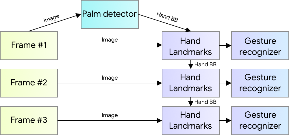
Our hand tracking solution utilizes an ML pipeline consisting of several models working together:
- A palm detector model (called BlazePalm) that operates on the full image and returns an oriented hand bounding box.
- A hand landmark model that operates on the cropped image region defined by the palm detector and returns high fidelity 3D hand keypoints.
- A gesture recognizer that classifies the previously computed keypoint configuration into a discrete set of gestures.
This architecture is similar to that employed by our recently published face mesh ML pipeline and that others have used for pose estimation. Providing the accurately cropped palm image to the hand landmark model drastically reduces the need for data augmentation (e.g. rotations, translation and scale) and instead allows the network to dedicate most of its capacity towards coordinate prediction accuracy.
 |
| Hand perception pipeline overview. |
BlazePalm: Realtime Hand/Palm Detection
To detect initial hand locations, we employ a single-shot detector model called BlazePalm, optimized for mobile real-time uses in a manner similar to BlazeFace, which is also available in MediaPipe. Detecting hands is a decidedly complex task: our model has to work across a variety of hand sizes with a large scale span (~20x) relative to the image frame and be able to detect occluded and self-occluded hands. Whereas faces have high contrast patterns, e.g., in the eye and mouth region, the lack of such features in hands makes it comparatively difficult to detect them reliably from their visual features alone. Instead, providing additional context, like arm, body, or person features, aids accurate hand localization.
Our solution addresses the above challenges using different strategies. First, we train a palm detector instead of a hand detector, since estimating bounding boxes of rigid objects like palms and fists is significantly simpler than detecting hands with articulated fingers. In addition, as palms are smaller objects, the non-maximum suppression algorithm works well even for two-hand self-occlusion cases, like handshakes. Moreover, palms can be modelled using square bounding boxes (anchors in ML terminology) ignoring other aspect ratios, and therefore reducing the number of anchors by a factor of 3-5. Second, an encoder-decoder feature extractor is used for bigger scene context awareness even for small objects (similar to the RetinaNet approach). Lastly, we minimize the focal loss during training to support a large amount of anchors resulting from the high scale variance.
With the above techniques, we achieve an average precision of 95.7% in palm detection. Using a regular cross entropy loss and no decoder gives a baseline of just 86.22%.
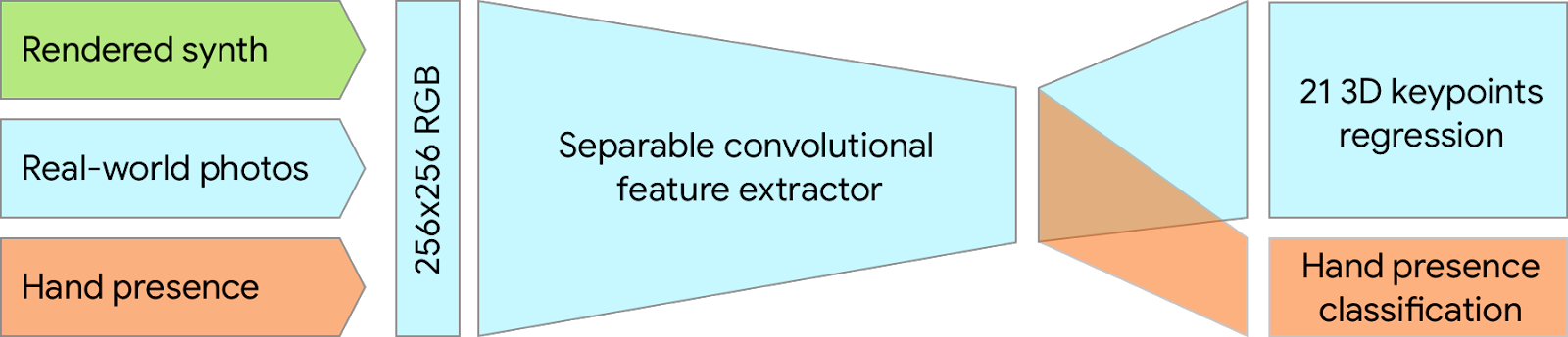
Hand Landmark Model
After the palm detection over the whole image our subsequent hand landmark model performs precise keypoint localization of 21 3D hand-knuckle coordinates inside the detected hand regions via regression, that is direct coordinate prediction. The model learns a consistent internal hand pose representation and is robust even to partially visible hands and self-occlusions.
To obtain ground truth data, we have manually annotated ~30K real-world images with 21 3D coordinates, as shown below (we take Z-value from image depth map, if it exists per corresponding coordinate). To better cover the possible hand poses and provide additional supervision on the nature of hand geometry, we also render a high-quality synthetic hand model over various backgrounds and map it to the corresponding 3D coordinates.
 |
| Top: Aligned hand crops passed to the tracking network with ground truth annotation. Bottom: Rendered synthetic hand images with ground truth annotation |
However, purely synthetic data poorly generalizes to the in-the-wild domain. To overcome this problem, we utilize a mixed training schema. A high-level model training diagram is presented in the following figure.
 |
| Mixed training schema for hand tracking network. Cropped real-world photos and rendered synthetic images are used as input to predict 21 3D keypoints. |
The table below summarizes regression accuracy depending on the nature of the training data. Using both synthetic and real world data results in a significant performance boost.
| Dataset | Mean regression error normalized by palm size |
| Only real-world | 16.1 % |
| Only rendered synthetic | 25.7 % |
| Mixed real-world + synthetic | 13.4 % |
Gesture Recognition
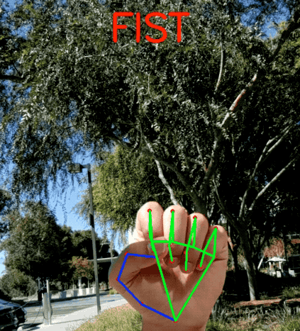
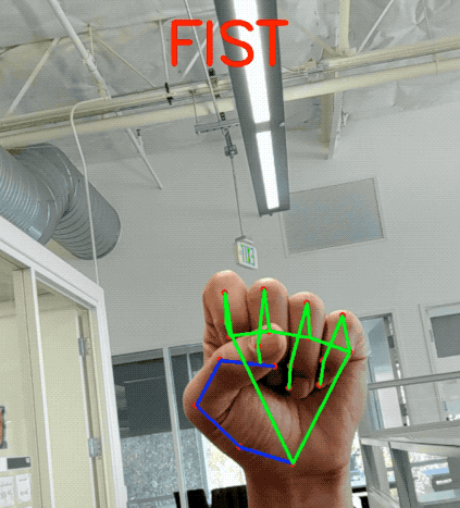
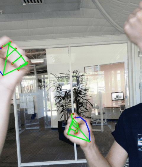
On top of the predicted hand skeleton, we apply a simple algorithm to derive the gestures. First, the state of each finger, e.g. bent or straight, is determined by the accumulated angles of joints. Then we map the set of finger states to a set of pre-defined gestures. This straightforward yet effective technique allows us to estimate basic static gestures with reasonable quality. The existing pipeline supports counting gestures from multiple cultures, e.g. American, European, and Chinese, and various hand signs including “Thumb up”, closed fist, “OK”, “Rock”, and “Spiderman”.
 |
 |
Implementation via MediaPipe
With MediaPipe, this perception pipeline can be built as a directed graph of modular components, called Calculators. Mediapipe comes with an extendable set of Calculators to solve tasks like model inference, media processing algorithms, and data transformations across a wide variety of devices and platforms. Individual calculators like cropping, rendering and neural network computations can be performed exclusively on the GPU. For example, we employ TFLite GPU inference on most modern phones.
Our MediaPipe graph for hand tracking is shown below. The graph consists of two subgraphs—one for hand detection and one for hand keypoints (i.e., landmark) computation. One key optimization MediaPipe provides is that the palm detector is only run as necessary (fairly infrequently), saving significant computation time. We achieve this by inferring the hand location in the subsequent video frames from the computed hand key points in the current frame, eliminating the need to run the palm detector over each frame. For robustness, the hand tracker model outputs an additional scalar capturing the confidence that a hand is present and reasonably aligned in the input crop. Only when the confidence falls below a certain threshold is the hand detection model reapplied to the whole frame.
 |
| The hand landmark model’s output (REJECT_HAND_FLAG) controls when the hand detection model is triggered. This behavior is achieved by MediaPipe’s powerful synchronization building blocks, resulting in high performance and optimal throughput of the ML pipeline. |
A highly efficient ML solution that runs in real-time and across a variety of different platforms and form factors involves significantly more complexities than what the above simplified description captures. To this end, we are open sourcing the above hand tracking and gesture recognition pipeline in the MediaPipe framework, accompanied with the relevant end-to-end usage scenario and source code, here. This provides researchers and developers with a complete stack for experimentation and prototyping of novel ideas based on our model.
Future Directions
We plan to extend this technology with more robust and stable tracking, enlarge the amount of gestures we can reliably detect, and support dynamic gestures unfolding in time. We believe that publishing this technology can give an impulse to new creative ideas and applications by the members of the research and developer community at large. We are excited to see what you can build with it!
Acknowledgements
Special thanks to all our team members who worked on the tech with us: Andrey Vakunov, Andrei Tkachenka, Yury Kartynnik, Artsiom Ablavatski, Ivan Grishchenko, Kanstantsin Sokal, Mogan Shieh, Ming Guang Yong, Anastasia Tkach, Jonathan Taylor, Sean Fanello, Sofien Bouaziz, Juhyun Lee, Chris McClanahan, Jiuqiang Tang, Esha Uboweja, Hadon Nash, Camillo Lugaresi, Michael Hays, Chuo-Ling Chang, Matsvei Zhdanovich and Matthias Grundmann.
What Is Conversational AI?
For a quality conversation between a human and a machine, responses have to be quick, intelligent and natural-sounding.
But up to now, developers of language-processing neural networks that power real-time speech applications have faced an unfortunate trade-off: Be quick and you sacrifice the quality of the response; craft an intelligent response and you’re too slow.
That’s because human conversation is incredibly complex. Every statement builds on shared context and previous interactions. From inside jokes to cultural references and wordplay, humans speak in highly nuanced ways without skipping a beat. Each response follows the last, almost instantly. Friends anticipate what the other will say before words even get uttered.
What Is Conversational AI?
True conversational AI is a voice assistant that can engage in human-like dialogue, capturing context and providing intelligent responses. Such AI models must be massive and highly complex.
But the larger a model is, the longer the lag between a user’s question and the AI’s response. Gaps longer than just two-tenths of a second can sound unnatural.
With NVIDIA GPUs and CUDA-X AI libraries, massive, state-of-the-art language models can be rapidly trained and optimized to run inference in just a couple of milliseconds, thousandths of a second — a major stride towards ending the tradeoff between an AI model that’s fast versus one that’s large and complex.
These breakthroughs help developers build and deploy the most advanced neural networks yet, and bring us closer to the goal of achieving truly conversational AI.
GPU-optimized language understanding models can be integrated into AI applications for such industries as healthcare, retail and financial services, powering advanced digital voice assistants in smart speakers and customer service lines. These high-quality conversational AI tools can allow businesses across sectors to provide a previously unattainable standard of personalized service when engaging with customers.
How Fast Does Conversational AI Have to Be?
The typical gap between responses in natural conversation is about 200 milliseconds. For an AI to replicate human-like interaction, it might have to run a dozen or more neural networks in sequence as part of a multilayered task — all within that 200 milliseconds or less.
Responding to a question involves several steps: converting a user’s speech to text, understanding the text’s meaning, searching for the best response to provide in context, and providing that response with a text-to-speech tool. Each of these steps requires running multiple AI models — so the time available for each individual network to execute is around 10 milliseconds or less.
If it takes longer for each model to run, the response is too sluggish and the conversation becomes jarring and unnatural.
Working with such a tight latency budget, developers of current language understanding tools have to make tradeoffs. A high-quality, complex model could be used as a chatbot, where latency isn’t as essential as in a voice interface. Or, developers could rely on a less bulky language processing model that more quickly delivers results, but lacks nuanced responses.
What Will Future Conversational AI Sound Like?
Basic voice interfaces like phone tree algorithms (with prompts like “To book a new flight, say ‘bookings’”) are transactional, requiring a set of steps and responses that move users through a pre-programmed queue. Sometimes it’s only the human agent at the end of the phone tree who can understand a nuanced question and solve the caller’s problem intelligently.
Voice assistants on the market today do much more, but are based on language models that aren’t as complex as they could be, with millions instead of billions of parameters. These AI tools may stall during conversations by providing a response like “let me look that up for you” before answering a posed question. Or they’ll display a list of results from a web search rather than responding to a query with conversational language.
A truly conversational AI would go a leap further. The ideal model is one complex enough to accurately understand a person’s queries about their bank statement or medical report results, and fast enough to respond near instantaneously in seamless natural language.
Applications for this technology could include a voice assistant in a doctor’s office that helps a patient schedule an appointment and follow-up blood tests, or a voice AI for retail that explains to a frustrated caller why a package shipment is delayed and offers a store credit.
Demand for such advanced conversational AI tools is on the rise: an estimated 50 percent of searches will be conducted with voice by 2020, and, by 2023, there will be 8 billion digital voice assistants in use.
What Is BERT?
BERT (Bidirectional Encoder Representations from Transformers) is a large, computationally intensive model that set the state of the art for natural language understanding when it was released last year. With fine-tuning, it can be applied to a broad range of language tasks such as reading comprehension, sentiment analysis or question and answer.
Trained on a massive corpus of 3.3 billion words of English text, BERT performs exceptionally well — better than an average human in some cases — to understand language. Its strength is its capability to train on unlabeled datasets and, with minimal modification, generalize to a wide range of applications.
The same BERT can be used to understand several languages and be fine-tuned to perform specific tasks like translation, autocomplete or ranking search results. This versatility makes it a popular choice for developing complex natural language understanding.
At BERT’s foundation is the Transformer layer, an alternative to recurrent neural networks that applies an attention technique — parsing a sentence by focusing attention on the most relevant words that come before and after it.
The statement “There’s a crane outside the window,” for example, could describe either a bird or a construction site, depending on whether the sentence ends with “of the lakeside cabin” or “of my office.” Using a method known as bidirectional or nondirectional encoding, language models like BERT can use context cues to better understand which meaning applies in each case.
Leading language processing models across domains today are based on BERT, including BioBERT (for biomedical data), SciBERT (for scientific publications) and ERNIE (which incorporates knowledge graphs for better language understanding).
How Does NVIDIA Technology Optimize Transformer-Based Models?
The parallel processing capabilities and Tensor Core architecture of NVIDIA GPUs allow for higher throughput and scalability when working with complex language models — enabling record-setting performance for both the training and inference of BERT.
Using the powerful NVIDIA DGX SuperPOD system, the 340 million-parameter BERT-Large model can be trained in under an hour, compared to a typical training time of several days. But for real-time conversational AI, the essential speedup is for inference.
NVIDIA developers optimized the 110 million-parameter BERT-Base model for inference using TensorRT software. Running on NVIDIA T4 GPUs, the model was able to compute responses in just 2.2 milliseconds when tested on the Stanford Question Answering Dataset. Known as SQuAD, the dataset is a popular benchmark to evaluate a model’s ability to understand context.
The latency threshold for many real-time applications is 10 milliseconds. Even highly optimized CPU code results in a processing time of more than 40 milliseconds.
By shrinking inference time down to a couple milliseconds, it’s practical for the first time to deploy BERT in production. And it doesn’t stop with BERT — the same methods can be used to accelerate other large, Transformer-based natural language models like GPT-2, XLNet and RoBERTa.
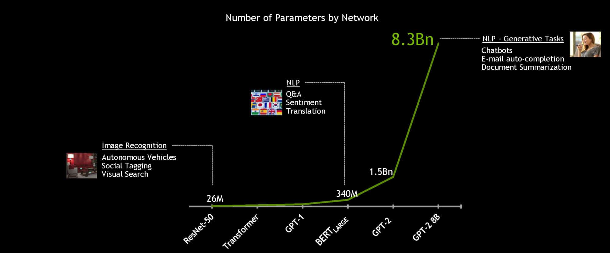
To work toward the goal of truly conversational AI, language models are getting larger over time. Future models will be many times bigger than those used today, so NVIDIA built and open-sourced the largest Transformer-based AI yet: GPT-2 8B, an 8.3 billion-parameter language processing model that’s 24x bigger than BERT-Large.
For more information on training BERT on GPUs, optimizing BERT for inference, and other projects in natural language processing, check out NVIDIA’s developer blog.
The post What Is Conversational AI? appeared first on The Official NVIDIA Blog.
Joint Speech Recognition and Speaker Diarization via Sequence Transduction
Being able to recognize “who said what,” or speaker diarization, is a critical step in understanding audio of human dialog through automated means. For instance, in a medical conversation between doctors and patients, “Yes” uttered by a patient in response to “Have you been taking your heart medications regularly?” has a substantially different implication than a rhetorical “Yes?” from a physician.
Conventional speaker diarization (SD) systems use two stages, the first of which detects changes in the acoustic spectrum to determine when the speakers in a conversation change, and the second of which identifies individual speakers across the conversation. This basic multi-stage approach is almost two decades old, and during that time only the speaker change detection component has improved.
With the recent development of a novel neural network model—the recurrent neural network transducer (RNN-T)—we now have a suitable architecture to improve the performance of speaker diarization addressing some of the limitations of the previous diarization system we presented recently. As reported in our recent paper, “Joint Speech Recognition and Speaker Diarization via Sequence Transduction,” to be presented at Interspeech 2019, we have developed an RNN-T based speaker diarization system and have demonstrated a breakthrough in performance from about 20% to 2% in word diarization error rate—a factor of 10 improvement.
Conventional Speaker Diarization Systems
Conventional speaker diarization systems rely on differences in how people sound acoustically to distinguish the speakers in the conversations. While male and female speakers can be identified relatively easily from their pitch using simple acoustic models (e.g., Gaussian mixture models) in a single stage, speaker diarization systems use a multi-stage approach to distinguish between speakers having potentially similar pitch. First, a change detection algorithm breaks up the conversation into homogeneous segments, hopefully containing only a single speaker, based upon detected vocal characteristics. Then, deep learning models are employed to map segments from each speaker to an embedding vector. Finally, in a clustering stage, these embeddings are grouped together to keep track of the same speaker across the conversation.
In practice, the speaker diarization system runs in parallel to the automatic speech recognition (ASR) system and the outputs of the two systems are combined to attribute speaker labels to the recognized words.
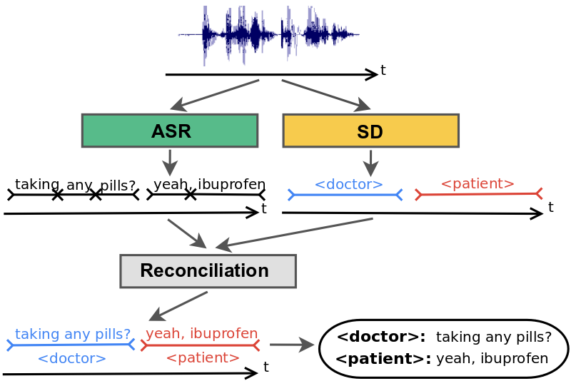 |
| Conventional speaker diarization system infers speaker labels in the acoustic domain and then overlays the speaker labels on the words generated by a separate ASR system. |
There are several limitations with this approach that have hindered progress in this field. First, the conversation needs to be broken up into segments that only contain speech from one speaker. Otherwise, the embedding will not accurately represent the speaker. In practice, however, the change detection algorithm is imperfect, resulting in segments that may contain multiple speakers. Second, the clustering stage requires that the number of speakers be known and is particularly sensitive to the accuracy of this input. Third, the system needs to make a very difficult trade-off between the segment size over which the voice signatures are estimated and the desired model accuracy. The longer the segment, the better the quality of the voice signature, since the model has more information about the speaker. This comes at the risk of attributing short interjections to the wrong speaker, which could have very high consequences, for example, in the context of processing a clinical or financial conversation where affirmation or negation needs to be tracked accurately. Finally, conventional speaker diarization systems do not have an easy mechanism to take advantage of linguistic cues that are particularly prominent in many natural conversations. An utterance, such as “How often have you been taking the medication?” in a clinical conversation is most likely uttered by a medical provider, not a patient. Likewise, the utterance, “When should we turn in the homework?” is most likely uttered by a student, not a teacher. Linguistic cues also signal high probability of changes in speaker turns, for example, after a question.
There are a few exceptions to the conventional speaker diarization system, but one such exception was reported in our recent blog post. In that work, the hidden states of the recurrent neural network (RNN) tracked the speakers, circumventing the weakness of the clustering stage. Our approach takes a different approach and incorporates linguistic cues, as well.
An Integrated Speech Recognition and Speaker Diarization System
We developed a novel and simple model that not only combines acoustic and linguistic cues seamlessly, but also combines speaker diarization and speech recognition into one system. The integrated model does not degrade the speech recognition performance significantly compared to an equivalent recognition only system.
The key insight in our work was to recognize that the RNN-T architecture is well-suited to integrate acoustic and linguistic cues. The RNN-T model consists of three different networks: (1) a transcription network (or encoder) that maps the acoustic frames to a latent representation, (2) a prediction network that predicts the next target label given the previous target labels, and (3) a joint network that combines the output of the previous two networks and generates a probability distribution over the set of output labels at that time step. Note, there is a feedback loop in the architecture (diagram below) where previously recognized words are fed back as input, and this allows the RNN-T model to incorporate linguistic cues, such as the end of a question.
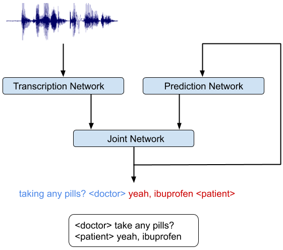 |
| An integrated speech recognition and speaker diarization system where the system jointly infers who spoke when and what. |
Training the RNN-T model on accelerators like graphical processing units (GPU) or tensor processing units (TPU) is non-trivial as computation of the loss function requires running the forward-backward algorithm, which includes all possible alignments of the input and the output sequences. This issue was addressed recently in a TPU friendly implementation of the forward-backward algorithm, which recasts the problem as a sequence of matrix multiplications. We also took advantage of an efficient implementation of the RNN-T loss in TensorFlow that allowed quick iterations of model development and trained a very deep network.
The integrated model can be trained just like a speech recognition system. The reference transcripts for training contain words spoken by a speaker followed by a tag that defines the role of the speaker. For example, “When is the homework due?” ≺student≻, “I expect you to turn them in tomorrow before class,” ≺teacher≻. Once the model is trained with examples of audio and corresponding reference transcripts, a user can feed in the recording of the conversation and expect to see an output in a similar form. Our analyses show that improvements from the RNN-T system impact all categories of errors, including short speaker turns, splitting at the word boundaries, incorrect speaker assignment in the presence of overlapping speech, and poor audio quality. Moreover, the RNN-T system exhibited consistent performance across conversation with substantially lower variance in average error rate per conversation compared to the conventional system.
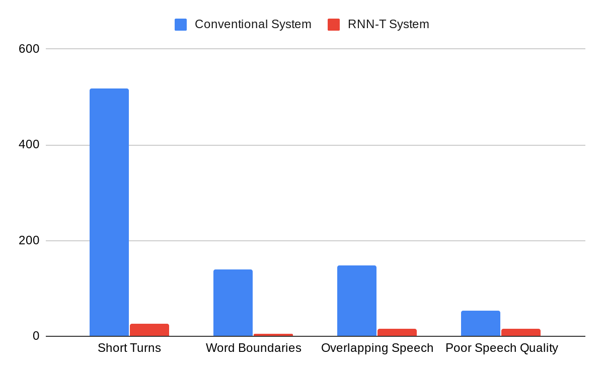 |
| A comparison of errors committed by the conventional system vs. the RNN-T system, as categorized by human annotators. |
Furthermore, this integrated model can predict other labels necessary for generating more reader-friendly ASR transcripts. For example, we have been able to successfully improve our transcripts with punctuation and capitalization symbols using the appropriately matched training data. Our outputs have lower punctuation and capitalization errors than our previous models that were separately trained and added as a post-processing step after ASR.
This model has now become a standard component in our project on understanding medical conversations and is also being adopted more widely in our non-medical speech services.
Acknowledgements
We would like to thank Hagen Soltau without whose contributions this work would not have been possible. This work was performed in collaboration with Google Brain and Speech teams.