
Blog

Learn About Our Meetup

5000+ Members

MEETUPS

LEARN, CONNECT, SHARE

Join our meetup, learn, connect, share, and get to know your Toronto AI community. 

JOB POSTINGS

INDEED POSTINGS

Browse through the latest deep learning, ai, machine learning postings from Indeed for the GTA.

CONTACT

CONNECT WITH US

Are you looking to sponsor space, be a speaker, or volunteer, feel free to give us a shout.

Category: Amazon

Developers, start your engines and get ready to race in the 2019 AWS DeepRacer League

Get ready to take the pole position in the AWS DeepRacer League. Today, we’re excited to bring you the next stage in the AWS DeepRacer journey – the AWS DeepRacer League 2019.

In November 2018, Jeff Barr announced the launch of AWS DeepRacer on the AWS News Blog as a new way to learn machine learning (ML). With AWS DeepRacer, developers have an opportunity to get hands-on with a fully autonomous 1/18th scale race car driven by reinforcement learning, a 3D racing simulator, and a global racing league.

Thousands of developers joined the live action at the race tracks at AWS re:Invent 2018, racing for glory and prizes, and to win the coveted AWS DeepRacer Championship Cup. The 2018 reigning Champion is Rick Fish, co-founder of UK-based FinTech startup Jigsaw XYZ. It was a close race, but Rick rose victorious with a winning lap time of 50.51 seconds. You can check out the final race and also a recent interview with Rick where he gave us an update on what he and his race team are doing to prepare to defend the title in the 2019 Championship, on deepracerleague.com.

Now it’s your turn to get on the track and learn ML with AWS DeepRacer. There are two ways to participate in the AWS DeepRacer League 2019: the Summit Circuit and the Virtual Circuit. Winners and top point scorers will be heading on an expenses-paid trip to race in the final stages of competition at AWS re:Invent 2019 in Las Vegas.

Summit Circuit – Bringing the race to a city near you

You can join us at any of the 20 AWS Summits, globally, where we help you build and train a model at a workshop, or you can bring a model you have trained at home. You can then put your model to the test and compete on the track in the AWS Summit Expo. There are no limits on how many of the 20 Summit events you can participate in. Simply register for the Summit you want to race at, and we will see you there. Check out the Summit Circuit schedule here.

Virtual Circuit – Compete from anywhere in the world

The Virtual Circuit opens up the race to anyone, anywhere. You can build models and compete online in the league through the AWS DeepRacer console. The virtual races will take place monthly on new, increasingly challenging tracks, and are open to all levels of expertise. Sign up for the preview to get on the list for early access. The first event of the Virtual Circuit will launch soon, stay tuned for updates on deepracerleague.com.

Whether you are new to machine learning or ready to build on your existing skills, we can help you get ready to race. Developers with no prior machine learning experience can get started by watching this AWS DeepRacer Tech Talk to get familiar with the basics of reinforcement learning (a branch of machine learning that’s ideal for training autonomous vehicles) and AWS DeepRacer. For the early adopters out there who are already comfortable with reinforcement learning, you can dive in and build an AWS DeepRacer model using the Amazon SageMaker RL notebook.

Come join us at one of the Summits or on the Virtual Circuit and get in on the action. It could be you lifting the Championship Cup in 2019. You can also follow the action online at deepracer.com and on Instagram: awsdeepracer.

Developers, the race is on!


About the Author

Sally Revell is a Principal Product Marketing Manager for AWS DeepLens. She loves to work on innovative products that have the potential to impact people’s lives in a positive way. In her spare time, she loves to do yoga, horseback riding and being outdoors in the beauty of the Pacific Northwest.


De-identify medical images with the help of Amazon Comprehend Medical and Amazon Rekognition

Medical images are a foundational tool in modern medicine that enable clinicians to visualize critical information about a patient to help diagnose and treat them. The digitization of medical images has vastly improved our ability to reliably store, share, view, search, and curate these images to assist our medical professionals. The number of modalities for medical images has also increased. From CT scans to MRIs, digital pathology to ultrasounds, there are vast amounts of medical data collected in medical image archives.

These medical images are also useful for medical research. Using machine learning, scientists at global medical research institutions can analyze hundreds of thousands or millions of images to deepen their insight into medical issues. The challenge for health professionals is how to use these images while complying with regulatory obligations like the Health Information Portability and Accountability Act (HIPAA). Often, medical images contain Protected Health Information (PHI) stored as text within the image itself. This has historically presented a challenge because the process of removing PHI, called de-identifying, required the manual review and editing of images. This manual process can easily take many minutes per image and makes de-identifying large datasets time consuming and expensive.

In 2017, Amazon Web Services (AWS) announced the ability to easily detect and extract text from images using our machine learning service Amazon Rekognition. In 2018, we announced a new machine learning Natural Language Processing (NLP) service for medical text called Amazon Comprehend Medical that can help customers to detect and identify PHI in a string of text. You can use these two services, plus some Python code, as demonstrated in this blog post, to inexpensively and quickly detect, identify, and redact PHI from within medical images.

De-identification architecture

In this example, we will use the Jupyter Notebooks feature of Amazon SageMaker to create an interactive notebook with Python code. Amazon SageMaker is an end-to-end machine learning platform that enables you to prepare training data and build machine learning models quickly using pre-built Jupyter notebook with pre-built algorithms. In this blog post, for the actual machine learning and prediction, we will be using Amazon Rekognition to extract text from the images and Amazon Comprehend Medical to help us to identify and detect the PHI. All of our image files will be read from and written to a bucket in Amazon Simple Storage Service (Amazon S3), an object storage service that offers industry-leading scalability, data availability, security, and performance.

When using Amazon Comprehend Medical to detect and identify protected health information, note that the service provides confidence scores for each identified entity that indicate the level of confidence in the accuracy of the detected entity. You should take these confidence scores into account and review identified entities to make sure they are correct and appropriate for your use case.  For more information about confidence scores, see the Amazon Comprehend Medical documentation.

Using the notebook

You can download the Jupyter Notebook that supports this blog post from GitHub.

This notebook shows an example chest x-ray image from a dataset made available by the NIH Clinical Center. The dataset can be downloaded from this link. See the NIH Clinical Center’s CVPR 2017 paper for more information.

At the very beginning of the notebook, you will see 5 parameters you can adjust to control the de-identification process outlined in this example.

  • bucket defines the Amazon S3 bucket where images will be read from and written to.
  • object defines the identified image that you want to de-identify. These can be PNG, JPG, or DICOM images. If the object ends with the extension .dcm, then the image is assumed to be a DICOM image, and the ImageMagick utility will be used to convert it to PNG format before processing it.
  • redacted_box_color defines the color that will be used to cover up identified PHI text within the image.
  • dpi defines the dpi setting that will be used in the output image.
  • phi_detection_threshold is the threshold for the confidence score mentioned earlier (between 0.00 and 1.00). Text detected and identified by Amazon Comprehend Medical must meet the minimum confidence score you set to be redacted from the output image. The default value of 0.00 will redact all text that Amazon Comprehend Medical has detected an identified as PHI, regardless of the confidence score.
#Define the S3 bucket and object for the medical image we want to analyze.  Also define the color used for redaction.
bucket='yourbucket'
object='yourimage.dcm'
redacted_box_color='red'
dpi = 72
phi_detection_threshold = 0.00

After these parameters are set, you can execute all of the cells in the Jupyter Notebook. The first cell converts the image file you specified from DICOM format to PNG, if necessary, and then reads the resulting file from S3 into memory.

#If the image is in DICOM format, convert it to PNG
if (object.split(".")[-1:][0] == "dcm"):
    ! aws s3 cp s3://{bucket}/{object} .
    ! mogrify -format png {object.split("/")[-1:][0]} {object.split("/")[-1:][0]}.png
    ! aws s3 cp {object.split("/")[-1:][0]}.png s3://{bucket}/{object}.png
    object=object+'.png'
    print(object)
…
#Download the image from S3 and hold it in memory
img_bucket = s3.Bucket(bucket)
img_object = img_bucket.Object(object)
xray = io.BytesIO()
img_object.download_fileobj(xray)
img = np.array(Image.open(xray), dtype=np.uint8)

From there, the image can be sent to Amazon Rekognition for text detection using the DetectText feature.  Amazon Rekognition returns a JSON object that contains a list of the text blocks detected within the image, as well as a bounding box that defines each text block, letting you know where the text is located within the image.

response=rekognition.detect_text(Image={'Bytes':xray.getvalue()})
textDetections=response['TextDetections']

After we have all of the text detected within the image, we can send that text to Amazon Comprehend Medical to determine which text blocks may contain PHI using the DetectPHI feature. Amazon Comprehend Medical then returns a JSON object containing the entities that may be PHI, a type that defines what kind of information it believes the text to be (name, date, address, ID), and a confidence score for each detection. We can use this to determine which bounding boxes contain PHI.

philist=comprehendmedical.detect_phi(Text = textblock)

After we know which areas of the image might contain PHI text, we can draw redacting boxes over those areas.

for box in phi_boxes_list:
    #The bounding boxes are described as a ratio of the overall image dimensions, so we must multiply them by the total image dimensions to get the exact pixel values for each dimension.
    x = img.shape[0] * box['Left']
    y = img.shape[1] * box['Top']
    width = img.shape[0] * box['Width']
    height = img.shape[1] * box['Height']
    rect = patches.Rectangle((x,y),width,height,linewidth=0,edgecolor=redacted_box_color,facecolor=redacted_box_color)
    ax.add_patch(rect)

The resulting de-identified image is then written to the S3 bucket that you specified, in PNG format, and with the text “de-id-“ prepended to the original file name.

Conclusion

This blog post has shown you the power and agility of using pre-trained machine learning models. It doesn’t take much development effort to combine AI services to accomplish complex tasks. When you use these services within a pre-configured machine learning development environment, such as Amazon SageMaker notebooks, you can execute your entire software development life cycle on fully managed infrastructure.

Running this example within an Amazon SageMaker notebook provides an ideal environment for you to understand the process used here and see the results. In addition, if you want to batch process thousands or millions of images, this same code could be implemented using AWS Lambda or AWS Batch. You could even associate a Lambda function containing this code with an Amazon S3 bucket so that every time a new image is added it would be de-identified.


About the Author

James Wiggins is a senior healthcare solutions architect at AWS. He is passionate about using technology to help organizations positively impact world health. He also loves spending time with his wife and three children.


Map clinical notes to the OMOP Common Data Model and healthcare ontologies using Amazon Comprehend Medical

Being able to describe the health of patients with observational data is an important aspect of our modern healthcare system. The amount of quantifiable personal health information is vast and constantly growing as new healthcare methods, metrics, and devices are introduced. All of this data allows clinicians and researchers to understand how the health of a patient changes over time and identify opportunities for precision treatment. The aggregate of this data informs epidemiologists about the health of populations and enables the identification of cause and effect patterns.

Unstructured text, commonly in the form of clinical notes, is a rich source of patient observational health data. Often, there is important information written by clinicians into notes that isn’t encoded into a patient’s structured health record. Clinical notes can also be used to help validate the quality of structured health record data. Historically, the challenge with clinical notes has been that they require manual review to extract the contained medical insights, which is time consuming and expensive.

Amazon Comprehend Medical is a natural language processing (NLP) service that uses machine learning to extract insights like medical condition, medication, dosage, and strength quickly and accurately. Customers can use Amazon Comprehend Medical in a pay-as-you-go model and immediately begin extracting insights from medical text without having to develop or train a complex machine learning model themselves.

The Observational Medical Outcomes Partnership (OMOP) Common Data Model, maintained by the Observational Health Data Science and Informatics (OHDSI) community, is an industry standard, open source data model used for health data. OMOP uses standardized medical ontologies, or “vocabularies,” like SNOMED, to store observational health data. From the OHDSI website:

“The OMOP Common Data Model allows for the systematic analysis of disparate observational databases. The concept behind this approach is to transform data contained within those databases into a common format (data model) as well as a common representation (terminologies, vocabularies, coding schemes), and then perform systematic analyses using a library of standard analytic routines that have been written based on the common format.”

A feature of OMOP is the ability to store clinical notes captured from disparate health data sources. In the data model, these notes are linked to an individual patient and a visit, giving context for the note. OMOP also has the ability to store insights inferred from notes by a natural language processing (NLP) engine. In this blog post we’ll explore how you can use Amazon Comprehend Medical to read notes from OMOP, extract medical insights, and write them back into OMOP using SNOMED ontological codes to enhance patient and population observational health data.

OMOP note processing architecture

This example works with clinical notes in the larger context of a full OHDSI architecture. You can learn more about our automated architecture for OHDSI on AWS by visiting this GitHub repository. The code given here specifically reads notes from and writes insights to the OMOP common data model. However, the same general process can be used with other structured data models for observational data that support clinical notes.

A primary feature of OMOP is the ability to consolidate data from many sources, like Electronic Health Record (EHR) systems and administrative claims data, from many geographic regions, into a common data model. In OMOP, the analysis of observational data from disparate sources is enabled by mapping dozens of source vocabularies (sometimes called dictionaries or ontologies) like SNOMED, RxNorm, ICD10, Read, LOINC, and others to an OMOP standard vocabulary. This enables OMOP to act as a kind of Rosetta stone to allow the interpretation of observational data between different sources and from different global regions.

One important aspect of the approach demonstrated here is mapping the entities detected by Amazon Comprehend Medical to the SNOMED ontology. Because observations must be expressed using standard codes in the OMOP data model, we must first map the insights detected by Amazon Comprehend Medical to a standard ontology before we can write them to OMOP. This is accomplished by sending entity text to the SNOMED CT Browser service to receive a SNOMED code for each entity. The following diagram shows the architecture for this process.


Using R code for notes processing

You can download the R Code demonstrating this process from GitHub.

This R code is demonstrated inside of the OHDSI on AWS architecture running on an Amazon EC2 instance running RStudio Server Open Source Edition instance. RStudio is a web-based, integrated development environment (IDE) for working with R. It can be licensed either commercially or under AGPLv3.

The code provided here can also be used from an environment outside of AWS to call Amazon Comprehend Medical. If you want to use it outside of AWS, you’ll need to configure a credentials file that allows this code to call the Amazon Comprehend Medical service. You can find instructions for doing that here.

At the very beginning of the notebook, you’ll see the following statements that define your OMOP CDM connection details and schema name. If you are using the OHDSI on AWS architecture, these are provided for you in a file called connectionDetails.R in your home directory. If outside of AWS, populate these lines with the details specific to your architecture.

#Source the DatabaseConnector::connect() call for my OMOP database
	connectionDetails <- DatabaseConnector::createConnectionDetails(
	dbms = "redshift",
	server = "myRedshiftClusterURL.us-east-1.redshift.amazonaws.com/mycdm",
	user = "master",
	password = "password")
cdmDatabaseSchema <- "CMSDESynPUF1k"

Amazon Comprehend Medical returns a confidence score for every entity, trait, and attribute that it detects. Next in the code, you’ll see a variable that defines a minimum confidence score that detections must meet in order to be written to the NOTE_NLP table. This minimum confidence score can be altered as appropriate for your use case.

#Set the minimum confidence score an inference must meet from Amazon Comprehend Medical to be added to the NOTE_NLP table.
min_score <- 0.80

The actual calls to Amazon Comprehend Medical are implemented using the AWS SDK for Python (boto3). An R library called “reticulate” is used to execute this Python code from within R, pass in the note text, and receive back the entity data detected by Amazon Comprehend Medical.

#Reticulate is used to run Python code from within R
library(reticulate)
...
#source the Python code to call Amazon Comprehend Medical
e <- environment()
reticulate::source_python('call_comprehend_medical.py', envir = e)

Every note found in the OMOP NOTE table is read using a SQL query and processed. For each entity detected in each note by Amazon Comprehend Medical, an appropriate SNOMED code is determined by calling the SNOMED CT Browser.

#Pass the detected medical entity to the SNOMED REST interface to get the matching SNOMED code.
snomed_call <- paste(base,endpoint,"?","query","=", entity$Text,"&limit=1&searchMode=partialMatching&lang=english&statusFilter=activeOnly&skipTo=0 &returnLimit=1&normalize=true", sep="")
get_snomed <- GET(snomed_call, type = "basic")

As each note is processed you’ll see output to the R console that shows each record written to the NOTE_NLP table.

[1] "Writing note_nlp record, 441... Standard Concept ID:313217, Lexical Variant: atrial fibrillation, Term Modifiers: CATEGORY: MEDICAL_CONDITION; TYPE: DX_NAME; TRAIT: DIAGNOSIS;"
  |=======================================================================================================================================| 100%
Executing SQL took 0.287 secs
[1] "Writing note_nlp record, 442... Standard Concept ID:4300877, Lexical Variant: left, Term Modifiers: CATEGORY: ANATOMY; TYPE: DIRECTION;"
  |=======================================================================================================================================| 100%
Executing SQL took 0.258 secs
[1] "Writing note_nlp record, 443... Standard Concept ID:4298444, Lexical Variant: breast, Term Modifiers: CATEGORY: ANATOMY; TYPE: SYSTEM_ORGAN_SITE;"
  |=======================================================================================================================================| 100%
Executing SQL took 0.259 secs
[1] "Writing note_nlp record, 444... Standard Concept ID:4112853, Lexical Variant: breast cancer, Term Modifiers: CATEGORY: MEDICAL_CONDITION; TYPE: DX_NAME; TRAIT: DIAGNOSIS;"
  |=======================================================================================================================================| 100%
Executing SQL took 0.45 secs
[1] "Writing note_nlp record, 445... Standard Concept ID:4080761, Lexical Variant: right, Term Modifiers: CATEGORY: ANATOMY; TYPE: DIRECTION;"
  |=======================================================================================================================================| 100%

After the processing is complete, you’ll have a NOTE_NLP table filled with records that represent medical insights extracted from the notes in your NOTE table. Each of these records has an OMOP Standard Concept ID (the NOTE_NLP_CONCEPT_ID field), mapped from a SNOMED code, that represents the primary entity detected. The TERM_MODIFIERS field in the NOTE_NLP table is used to capture the category, type, and any attribute or trait data that Amazon Comprehend Medical detected about each entity.

The following image shows a comparison of some original portions of note text with entities detected by Amazon Comprehend Medical and the corresponding NOTE_NLP record written to OMOP.

Conclusion

This example shows how Amazon Comprehend Medical makes natural language processing for medical text easily accessible. The insights detected by Amazon Comprehend Medical enable data scientists, epidemiologists, and medical researchers to extend patient and population structured observational health records with information that is locked away in unstructured notes. This additional data provides important insight for precision medicine, longitudinal studies, clinical trial candidate assessment, and population health studies. The code given here can help you get started processing notes into the OMOP Common Data Model today, or it can be used as a pattern to process clinical notes into any observational health data model.


About the Author

James Wiggins is a senior healthcare solutions architect at AWS. He is passionate about using technology to help organizations positively impact world health. He also loves spending time with his wife and three children.


Become a certified machine learning developer with the new AWS Certified Machine Learning – Specialty certification

Back in November 2018 we announced on this blog that the same machine learning (ML) courses used to train engineers at Amazon are now available to all developers through AWS. Today, we’re letting you know that there is a way to enhance and validate your ability to build, train, tune, and deploy machine learning models with AWS.

AWS Training and Certification is excited to announce the availability of the new AWS Certified Machine Learning – Specialty certification. This new exam was created by AWS experts for developers and data scientists who want to validate their ability to design, implement, deploy, and maintain ML solutions for given business problems. In addition, it validates their ability to select and justify the appropriate ML approach for a given business problem, identify appropriate AWS services to implement ML solutions, and design and implement scalable, cost-optimized, reliable, and secure ML solutions. AWS Training and Certification recommends one or more years of hands-on experience using ML  and artificial intelligence (AI) services, particularly Amazon SageMaker, and other services such as Amazon EMR, AWS Lambda, AWS Glue, and Amazon S3. It is also encouraged, but not required, that candidates hold an Associate-level certification or the Cloud Practitioner certification.

I had a chance to catch up with Swami Sivasubramanian, who is the Vice President of Machine Learning at AWS, to hear his thoughts on the needs in this growing field. “Customers tell us that they need more skilled talent in the area of machine learning, which has been a familiar problem within Amazon as well. It’s why we invested so deeply in creating internal education to train developers on machine learning,” he said. “AWS Training and Certification is helping to put those same resources in the hands of our customers so that they can develop and validate skills among their staff which will enable them to take full advantage of the growing AI/ML suite from AWS and the transformational effect that this technology will have on organizations and the global economy.”

Your ability to build, train, tune, and deploy ML models opens up many opportunities for new business ideas, new employment opportunities, and new customer experiences. Are you ready to get started?

Next Steps

The exam is available in English and Japanese at testing centers worldwide for $300 USD. You can learn more about the exam here. AWS offers an exam guide which provides training resources and materials to help you prepare. In addition, a learning path, called “Exam Preparation,” specifically designed for those taking the exam is available at aws.training/machinelearning.


– Maureen Lonergan – Director, AWS Training and Certification

Model serving with Amazon Elastic Inference

Amazon Elastic Inference (EI) is a service that allows you to attach low-cost GPU-powered acceleration to Amazon EC2 and Amazon SageMaker instances. EI reduces the cost of running deep learning inference by up to 75%. Model Server for Apache MXNet (MMS) enables deployment of MXNet- and ONNX-based models for inference at scale. In this blog post, we’ll explore using MMS running on a general purpose EC2 instance with an Elastic Inference Accelerator (EIA) attached.

What is Model Server for Apache MXNet (MMS)?

MMS is an open-source model serving framework designed to simplify the task of serving deep learning models for inference at scale. After training deep learning models using Apache MXNet, MMS makes it easy to deploy the trained model for inference at scale in a production environment. The following architectural diagram shows a standard MMS scalable architecture.

What is Amazon Elastic Inference?

In deep learning applications, inference drives as much as 90 percent of the compute costs of the application. Accelerated GPU instances are oversized for inference because inference happens on a single input in real time that consumes only a small amount of GPU compute. GPU compute capacity usage might not be 100 percent even at peak load, which is wasteful and costly.

EI allows you to attach just the right amount of GPU-powered inference acceleration to any EC2 or Amazon SageMaker instance and save up to 75 percent. With EI, you can now choose the instance type that is best suited to the overall CPU and memory needs of your application, and then you can separately configure the amount of inference acceleration that you need to use resources efficiently and to reduce costs.

Setting up Amazon Elastic Inference with EC2

Starting up an EC2 instance with an attached EI accelerator requires some pre-configuration steps to setup your AWS account. Then, we can launch an instance with an accelerator by following the instructions in the Elastic Inference documentation. Here we’ll use a plain Ubuntu Amazon Machine Image (AMI), and configure it for our needs.

Serving ResNet-152 model with Elastic Inference

After launching an EC2 instance with an EI accelerator, we install MMS and the EI enabled version of MXNet.

# Install MMS 
$ pip install --user mxnet-model-server

# Install EIA enabled MXNet
$ wget https://s3.amazonaws.com/amazonei-apachemxnet/amazonei_mxnet-1.3.0-py2.py3-none-manylinux1_x86_64.whl
$ pip install --user amazonei_mxnet-1.3.0-py2.py3-none-manylinux1_x86_64.whl

Next, let’s start MMS with a ResNet-152 model-archive that is already configured for EI. To build your own model-archive with EIA support refer to Custom Service and Model Serving with Elastic Inference documentation. We configure MMS using a curl command to set the number of workers to 1, and to use synchronous creation of workers.

# Start MMS with resnet-152
$ mxnet-model-server --start --models resnet-152=https://s3.amazonaws.com/model-server/model_archive_1.0/resnet-152-eia.mar

# Scale to a single worker, make scale request call synchronous (by default the call is asynchronous)
$ curl -X PUT '127.0.0.1:8081/models/resnet-152?min_worker=1&synchronous=true'

Notice that we set min_worker=1 in the previous curl command to configure MMS. This is important for MMS on EI because inference calls to the EI accelerator are sequential, so we don’t gain much benefit from using more than one worker. Now the model is ready for some inference requests. To classify an image of a kitten, execute the following commands:

# Download Kitten image for classification
$ curl -O https://s3.amazonaws.com/model-server/inputs/kitten.jpg

# Run inference request using EIA
$ curl -X POST http://127.0.0.1:8080/predictions/resnet-152 -T kitten.jpg

This yields the following prediction results:

[
    {
      "probability": 0.7148934602737427,
      "class": "n02123045 tabby, tabby cat"
    },
    {
      "probability": 0.22877734899520874,
      "class": "n02123159 tiger cat"
    },
    {
      "probability": 0.04032360762357712,
      "class": "n02124075 Egyptian cat"
    },
    {
      "probability": 0.008370809257030487,
      "class": "n02127052 lynx, catamount"
    },
    {
      "probability": 0.0006728142034262419,
      "class": "n02129604 tiger, Panthera tigris"
    }
  ]

You can see that ResNet-152 identified the tabby cat using Elastic Inference hosted with MMS.

Cost and performance benefits of serving with Elastic Inference

In model serving, performance is measured in terms of throughput (number of inferences per second) and latency (time for each inference). For CPU or GPU instances, the best latency is achieved with a single worker, but higher throughput is achieved by using one worker for each vCPU or GPU. We started with an m5.large instance and evaluated both throughput and latency optimized configurations. We achieved a throughput of 4.5 requests per second, and 244ms latency. The cost efficiency of this configuration for 100,000 requests is $0.59. Compare this to the throughput of 41.42 on a p3.2xlarge, 23ms latency, and cost efficiency of $2.05. This can be expensive for production use cases. So, let’s look at how Amazon Elastic Inference can help.

EI accelerators are currently available in three sizes: eia1.medium, eia1.large, and eia1.xlarge. Each has from 1 to 4 GB of memory and from 8 to 32 TFLOPS of compute.

We evaluated performance of this model with an eia1.medium accelerator and observed that larger instance sizes didn’t materially improve latency performance. Next, we tested the m5.large with different EI accelerator sizes. Inference calls with an eia1.large accelerator had lower latency than an eia1.medium, but were not more cost efficient. We use eia1.medium since it provides a good balance between performance and cost for the ResNet-152 model use case.

When optimizing for throughout, the m5.large + eia1.medium instance is 46 percent as fast a regular p3.2xlarge but is 84 percent more cost efficient. It is also 30 percent more cost efficient than a c5.xlarge, while also delivering 1.9x the throughput. The m5.large + eia1.medium provides 4.2x more throughput than just the m5.large alone, with 45 percent better cost efficiency. The following figure shows results when optimizing for maximum throughput.

When optimizing for latency, the m5.large + eia1.medium instance is 43 percent more cost efficient than a c5.xlarge instance, while having 2.4x lower latency. Compared to the m5.large alone, adding an eia1.medium improves cost efficiency by 44 percent with 4.4x better latency. The p3.2xlarge instance has 2.3x lower latency but costs 5.6x more than an m5.large + eia1.medium. The following figure shows results when optimizing for minimum latency.

Conclusion

To recap, in this blog post we showed that Elastic Inference provides the best cost efficiency for running inference at scale while optimizing for latency or throughput.

Learn more about MMS and contribute

Using Elastic Inference is one among many possibilities of hosting models with MMS. To learn more about MMS, start with our examples and documentation in the repository’s model zoo and documentation folder.

We welcome community participation including questions, requests, and contributions, as we continue to improve MMS. If you are using MMS already, we welcome your feedback via the repository’s GitHub issues. Head over to awslabs/mxnet-model-server to get started!


Appendix

The following table shows the specific configuration settings we used, and raw results we presented in this post.

Table 1: Raw Performance and Cost Results for ResNet-152.

Instance Type Optimized for # of workers *  # of OMP threads ** Hourly cost Cost Efficiency Latency (ms) Throughput (requests/sec)
m5.large Throughput 2 1 $ 0.10 $ 0.59 444 4.50
m5.large Latency 1 1 $ 0.10 $ 0.65 244 4.08
m5.large + eia.medium Both 1 1

$ 0.23


$ 0.33 52 19.08
c5.xlarge Throughput 4 1 $ 0.17 $ 0.47 400 9.95
c5.xlarge Latency 1 4 $ 0.17 $ 0.64 134 7.38
p3.2xlarge Both 1 N/A $ 3.06 $ 2.05 23 41.42

* Number of workers for the model –This can be tuned with management API of MMS.
** OMP_NUM_THREADS per worker – This indicates number of OpenMP threads per worker.

Typically, MMS automatically scales the number of workers to the number of vCPUs (for CPU instances) or to the number of GPUs (for GPU instances). However, we found for EI that using more than one worker didn’t give us any more throughput, and reduced the inference latency significantly. Thus, we use a single worker to get the best performance on EI. But for CPU or GPU instances, we achieve higher throughput by setting the number of workers to a larger value.

Notice that an additional configuration setting is needed to optimize for latency or throughput on CPU instances by setting the environment variable OMP_NUM_THREADS. MMS automatically sets this variable to 1 by default to optimize for throughput. However, we set this to 4 for c5.xlarge to optimize for latency. But your results might vary depending on the instance you choose and your optimization strategy.


About the Authors

Rakesh Vasudevan is a Software Development Engineer with AWS Deep Learning.He is passionate about  building scalable deep learning systems. In spare time, he enjoys gaming, cricket and hanging out with friends and family.


Denis Davydenko is an Engineering Manager with AWS Deep Learning. He focuses on building Deep Learning tools that enable developers and scientists to build intelligent applications. In his spare time he enjoys spending time with his family, playing poker and video games.


Sam Skalicky is a Software Engineer with AWS Deep Learning and enjoys building heterogeneous high performance computing systems. He is an avid coffee enthusiast and avoids hiking at all costs.


Easily perform bulk label quality assurance using Amazon SageMaker Ground Truth

In this blog post we’re going to walk you through an example situation where you’ve just built a machine learning system that labels your data at volume and you want to perform manual quality assurance (QA) on some of the labels. How can you do so without overwhelming your limited resources?  We’ll show you how, by using an Amazon SageMaker Ground Truth custom labeling job.

Rather than asking your workers to validate items one at a time, you’ll accomplish custom labeling by presenting a small batch of already-labeled items that have been assigned the same label. You’ll ask the worker to mark any that aren’t correct. In this way, a workforce is able to quickly assess a much larger quantity of data than they could label from scratch in the same time.

Use case tasks that might require quality assurance include:

  • Requiring subject matter expert review and approval of labels before using them for sensitive use cases.
  • Reviewing the labels to test the quality of the label-producing model.
  • Identifying and counting mislabeled items, correcting them, and feeding them back into the training set.
  • Analyzing label correctness versus confidence levels assigned by the model.
  • Understanding whether a single threshold can be applied to all label classes, or whether using different thresholds for different classes is more appropriate.
  • Exploring the use of a simpler model to label some initial data, then improving the model by using QA to validate the results and retrain.

In this blog post, you’ll walk through an example that addresses these use cases.

Background and solution overview

Amazon SageMaker Ground Truth offers easy access to public and private human labelers and provides them with built-in workflows and interfaces for common labeling tasks. In this blog post, you leverage and extend a Ground Truth Custom Labeling Workflow to support another time-consuming part of an overall system or business process: quality assurance of labels that have been applied, either via machine learning or by human labelers.

The input in this sample case is a list of labeled images to be validated by your private workforce. A worker sees a batch of images with a single label presented on a single screen, so they can validate a set of labels at a time. They can quickly scan the entire set and mark any that are not correctly labeled, picking out the ones that don’t “fit.” The validated results are stored in an Amazon DynamoDB table.  Note that the volume of items in a batch should be chosen appropriately for the task, depending on their complexity and ability to be displayed for easy comparison and review. For our example, the batch size was chosen as 25 (configurable in the template) to balance cognitive load with the volume of images to be reviewed.

Anatomy of an Amazon SageMaker Ground Truth custom labeling job

An Amazon SageMaker Ground Truth custom labeling workflow consists of the following components:

  • A workforce, to perform the labeling tasks. You can choose from a public workforce (for example, by using Amazon Mechanical Turk), or a private workforce.
  • A JSON manifest file. The manifest tells Ground Truth where to find the job inputs. Each line item is a single object and corresponds to a single task. In our example, each object is a custom labeling input that points to a batch of images with the same label that will be presented to the worker at the same time for QA.
  • A pre-labeling task AWS Lambda function. Before a labeling task is sent to the worker, your AWS Lambda pre-labeling function will be sent a JSON-formatted request to provide details. This JSON request must contain all the details the function will need in order to pass to the custom labeling job template.
  • A custom labeling task template. The template defines what will be shown to the worker during the labeling task. The inputs to the task are made available to the template by the pre-labeling task Lambda function.
  • A post-labeling task Lambda function. When the worker has completed the task, Ground Truth will send the results to your post-labeling task Lambda function. This Lambda function is generally used for annotation consolidation. The actual annotation data will be stored in a file designated by the s3Uri string in the payload object.

After these components are set up, you can create a Ground Truth labeling job that specifies these components. Ground Truth takes care of sending the individual labeling tasks to the workers and consolidating the outputs.

Solution overview

For the use case described in this blog post, the input to this process is images that have already been labeled by a machine learning model such as Amazon Rekognition, with a label and the confidence score the model had in assigning the label.

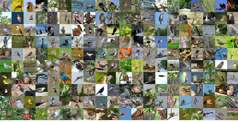
In this example, you’ll use a subset of the CalTech 101[i] dataset from AWS Open Datasets for image classification, which we’ve prelabeled for you. A corpus input file has been provided that specifies the subset of images to use and their labels. For example, our model had taken the following images and labeled them as “Crawdad”:

images/crayfish-image_0002.jpg,Crawdad,99.73238372802734
images/crayfish-image_0003.jpg,Crawdad,94.8296127319336
images/crayfish-image_0004.jpg,Crawdad,99.267822265625

Now, you’re interested in assessing the quality of the labels that have been applied.

The following diagram shows the overall process flow.

  1. In steps 1, 2 and 3, users identify images and upload them.
  2. In step 4, a model analyzes the images and labels them (step 5).
  3. In step 6, labels and images are aggregated and Ground Truth labeling jobs created.
  4. A workforce of labelers reviews the labels in step 7.
  5. In step 8a, the results are sent back to the model for retraining.
  6. In step 8b, the results are analyzed by data scientists to better understand model behavior, and by the business to understand how the model’s inferences in the production system should be best used.

In the remainder of this blog post, we’ll walk you through an implementation that focuses on steps 6 and 7. You’ll also look at the results, step 8b.

Using the Amazon SageMaker Ground Truth custom labeling job for QA

In this section you’ll set up and execute the implementation components, shown in the figure that follows. The solution implementation uses two major components:

  1. An Amazon SageMaker Ground Truth custom labeling workflow.
  2. An Amazon DynamoDB table, used to store the results of the labeling task.

For ease of use, a Lambda function prepopulates an Amazon S3 bucket and an Amazon DynamoDB table for you.

You’ll execute the following steps:

  1. First, you’ll create a private workforce (1), using the AWS Management Console.
  2. Then, you’ll execute a provided AWS CloudFormation stack to set up resources: the Amazon S3 bucket containing job inputs, a DynamoDB table to hold the results, and the Pre-Labeling and Post-Labeling Lambda functions for use by Ground Truth. The stack will also run a Lambda function (Launch) to pre-populate the job manifests (2).
  3. You’ll create a Ground Truth labeling job that reads the manifest (3).
  4. Ground Truth then prepares the labeling tasks by sending them to the pre-labeling Lambda function and sends them to the workers (4).
  5. You’ll perform the label quality assurance step (5), acting as the private workforce (5).
  6. Ground Truth will send the worker-labeled data to the post-labeling Lambda function (6), which writes the worker-assigned labels to the DynamoDB label table (7)
  7. Lastly, you’ll review the results of the labeling task.

Here are the details. You can also see the source code here.

Create a private workforce

To set up your private workforce, use the AWS Management Console. Choose the Region us-east-1 (the workforce must be created in the Region where the code resides). Follow the instructions under “Creating a workforce using the console” under Managing a Private Workforce, using any of the three options presented. This step also creates a labeling portal sign-in URL. You’ll need this URL later.

Create a new team, called bulkQA. Add one worker: yourself. Add your email, and complete the registration step.

Set up resources

To see this solution in operation in us-west-2, choose the Launch Stack button that follows.

Cost: Note that the total solution costs around $1.00 to run. Remember to delete the CloudFormation stack when you’ve finished with the solution.

Choose Next. Check that the parameters shown in the following screenshot will work for your environment.

Finally, review all the settings on the next page. Select the box marked I acknowledge that AWS CloudFormation might create IAM resources (this is required since the script creates IAM resources), then choose Create.

Wait until the stack launch is  complete, and look at the stack Outputs tab.

You’ll see the stack has created the following resources:

  1. An Amazon Simple Storage Service (S3)bucket (key = BulkQABucket). This bucket now contains:
    1. A JSON file, manifest.json, that has been generated for you. This file contains a list of the custom labeling inputs. Each of these custom labeling inputs will become a separate Ground Truth labeling task within the overall labeling job.
    2. A series of folders containing images. These folders contain a batch of images that have been copied from the CalTech 101 dataset, for use during this labeling project.
    3. A folder called custom_labeling_inputs. This folder contains a set of JSON files that have been generated for you. Each file contains a batch of images that have been assigned the same label, along with the confidence the model had in that label, and the S3 location of the source image. For example:
      [{"s3_image_url": "s3://bulkqa-rbulkqas3bucket-13skff6csrdy9/images/dalmatian-image_0001.jpg", "label": "Dog", "confidence": "87.27241516113281"}, {"s3_image_url": "s3://bulkqa-rbulkqas3bucket-13skff6csrdy9/images/dalmatian-image_0002.jpg", "label": "Dog", "confidence": "93.71725463867188"}, {"s3_image_url": "s3://bulkqa-rbulkqas3bucket-13skff6csrdy9/images/dalmatian-image_0003.jpg", "label": "Dog", "confidence": "93.47685241699219"}, {"s3_image_url": "s3://bulkqa-rbulkqas3bucket-13skff6csrdy9/images/dalmatian-image_0004.jpg", "label": "Dog", "confidence": "93.66221618652344"}, {"s3_image_url": "s3://bulkqa-rbulkqas3bucket-13skff6csrdy9/images/dalmatian-image_0006.jpg", "label": "Dog", "confidence": "93.04904174804688"}]

    Each custom labeling input will become a single task in Ground Truth (subject to the chosen batch size) that shows all images listed in the array along with the label to the worker for confirmation.

  2. An AWS Identity and Access Management (IAM) role (key = SageMakerRoleARN), to be used by the Ground Truth custom labeling job.
  3. A DynamoDB table (key = DynamoDBLabelTableName). The table has been preloaded with the list of images on S3, the label, and the label confidence assigned by the source labeling model. These are the labels that you want to confirm.

In addition, the stack has created three Lambda functions. They are:

  1. rLambdaLaunchFunction. This Lambda function is run one time during the CloudFormation stack launch, to set up the environment for this use case. It takes as input a CSV file that contains three columns: image filename, label, and confidence. For each line item, it copies the image file to S3. It also creates an entry for that line item in DynamoDB, and creates the manifest files.
  2. rLambdaGTPreLabelingFunction. This Lambda function is run at the beginning of each custom labeling task. As input, it receives from Ground Truth the S3 URI of one of the custom labeling inputs. It reads the manifest from S3 and passes the contents to Ground Truth, wrapped in a JSON object:
    { "taskInput": { "sourceRef" : custom_labeling_input} } 

  3. rLambdaGTPostLabelingFunction. This Lambda function is run after a labeling task has been completed and consolidates the worker’s annotations. In this case, it simply reads the worker’s annotations and updates them in the DynamoDB table.

Now that these components have been created, you’re ready to create the custom labeling job.

Create the custom labeling job

In the AWS Management Console, go to the Amazon SageMaker console. In the left navigation bar, choose Ground Truth, then choose Labeling Jobs. Choose Create Labeling Job.

  1. Name the job “BulkQATestJob”
  2. The input dataset is at s3://<BULKQA-BUCKET>/manifest.json
  3. Set your output dataset location to s3://<BULKQA-BUCKET>/output/
  4. For the IAM Role, choose to enter a custom Role ARN. Copy the ARN for the SageMakerExecutionRole generated by CFN here.
  5. Scroll down. Under Task Type, choose Custom.
  6. Choose Next.

On the Select workers and configure tool page:

  1. Under Workers, choose worker type of Private.
  2. Under Private teams, choose the team you set up previously.

Scroll down. Under Custom labeling task setup:

  1. Choose a template type of Custom.
  2. Copy and paste the full text of the bulkqa html template shown below.
    <script src="https://assets.crowd.aws/crowd-html-elements.js"></script>
    <style>
    .center {    text-align: center;
      border: 3px solid white;
    }
    .row {    display: flex;
      flex-wrap: wrap;
      padding: 0 4px;
    }
    /* Create five equal columns that sits next to each other */
    .column {    flex: 18%;
      padding: 0 4px;
    }
    </style>
    <crowd-form>
    <div class="center">
    <h1> Confirm that each image is correctly labelled as "{{ task.input.sourceRef[0].label }}"</h1>
    </div>
    <div class="row">
    {% assign length = task.input.sourceRef.size | minus: 1 %}
    {% for i in (0..length) %}
    <div class="column">
    <crowd-card
     image="{{ task.input.sourceRef[i].s3_image_url | grant_read_access }}">
     <div class="center">Confirm <crowd-checkbox checked="true" name="{{ task.input.sourceRef[i].label }}-{{i}}" value="Confirmed" /></div>
    </crowd-card>
    </div>
    {% endfor %}
    </div>
    </crowd-form>

    The code here is just a few lines in length. The crowd-form tag wraps the custom task code. It reads the label for this set from task.input.sourceRef[0].label and uses that text to create the page instruction. A for-loop then creates a crowd-card for each image listed in the input custom_labeling_input this task received as input, and places a pre-checked check box under each image.

  3. Under Pre-labeling task Lambda function, choose the LambdaGTPreLabelingFunction from the drop-down list.
  4. Under Post-labeling task Lambda function, choose the LambdaGTPostLabelingFunction from the drop-down list.
  5. Choose Submit.

Ground Truth now shows the job status as In progress, with a no (blank) labeled objects/total.

Wait for a few minutes while Ground Truth validates that your job works. After a few minutes, the Labeled objects/total column in the UI should change to contain a count, such as:  0 / 9. The total is the number of Ground Truth custom labeling inputs that your workers will QA. Here, each class label may be one or more images, depending on the size you chose for the QA batch size.

Now your workforce should start receiving labeling tasks within a few minutes.

Confirming the image labels

In the AWS Management Console left navigation bar, choose Ground Truth Labeling workforces. Choose the Private tab. Under the Private workforce summary, choose the Labeling portal sign-in URL.

Sign in with your workforce user name and password. You should see a job listed. If you don’t, wait a few more minutes and refresh the page. Repeat until the data labeling job becomes available.

Choose Start Working.

For each assigned task, the worker web page presents a set of images, each of which has been assigned the same label. In the first example image below, it is cat, in the second, crab. Each image has a Confirm check box below the image. These check boxes are checked by default.

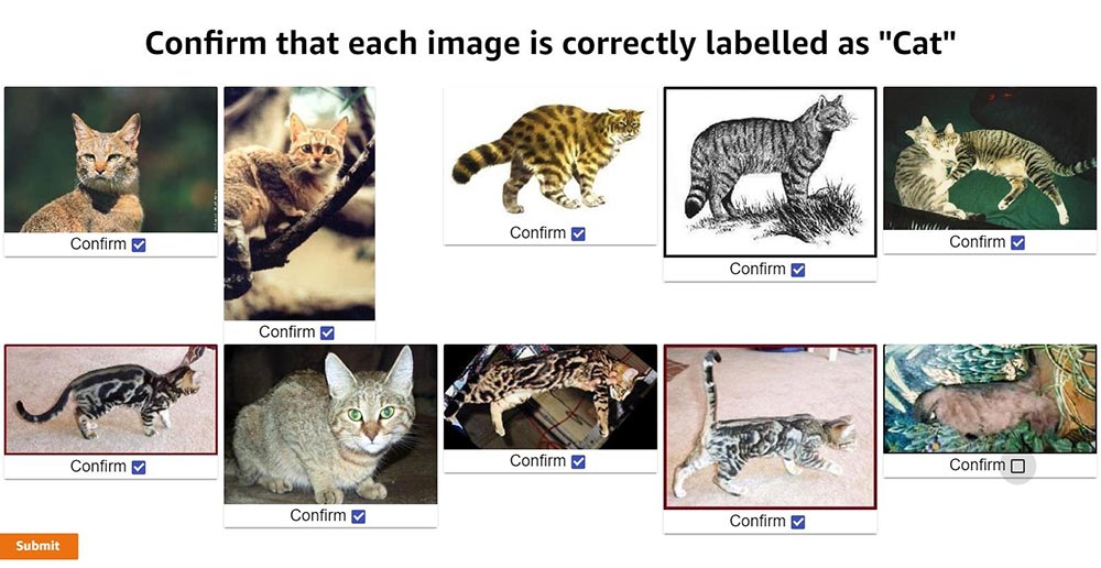
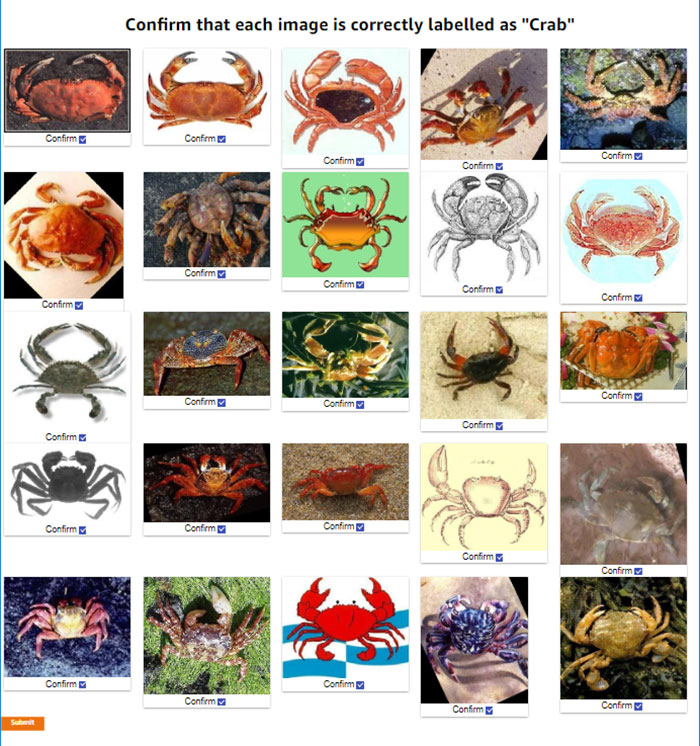
Review the images. For any image that does not match the label, uncheck the check box. When you’ve reviewed all the images on the page, choose Submit.

Behind the scenes, the post-labeling Lambda function runs. This Lambda function updates the DynamoDB table with the results. It adds up to two fields to each row: WorkerConfirmCount and WorkerDisconfirmCount. These columns are updated with the number of reviewers who have confirmed or disconfirmed each individual image.

Continue until all tasks have been completed. Ground Truth will batch the tasks, and then wait before assigning the next batch. If there are more than 10 tasks you will probably need to wait before the next batch becomes available to you.

Assessing the results

After all the tasks have been completed, the final results are ready for review in the DynamoDB table. In the AWS Management Console, navigate to the Amazon DynamoDB console. Under Tables, choose the BulkQALabelTable created earlier. Choose the Items tab, and review the table along with the worker confirmations.

In the screenshot of the DynamoDB console that follows, you can see that one worker has disconfirmed two of the images and has confirmed a third.

Having a single worker confirm the results might be reasonable if the worker is highly trained or otherwise considered an authoritative source of truth. Alternatively, for a sensitive use case or where your workers are less authoritative, you might want to have a larger number of workers – say, three – validate the results, and only use the ones that all have confirmed as correct.

Cleanup

After you have finished reviewing the results of this test, remember to delete the CloudFormation template. Doing so will remove the DynamoDB table and created S3 bucket, and prevent continuing charges.

Acting on the results

In this section we show you results from a specific assessment of the two larger samples. These were assessments from specific “experts,” so your results might vary. The two sample files are provided, and can be run by replacing bulkqa/smallsample.csv with their names in the CloudFormation template:

  • bulkqa/sample.csv contains 10 classes and 510 images
  • bulkqa/shellfish.csv contains 5 classes of shellfish, and 245 images.

These samples have more classes and more images, so they will take longer to assess. Ground Truth will send objects to your workers in batches. That is, it will assign some number of tasks – often 10 – to a worker, and then take a break before assigning the next set.

This method identifies false positives in any group. False negatives (images that should have been assigned to this class but were not) are not identified by this approach. You could add identifying the correct class (for example, out of a list of possible classes) to this method, at the cost of slowing down the QA process and potentially slowing down how quickly correctly classified items become available for use by the business. Alternatively, you could chain a separate process step that assigns the correct class for each misclassified item, for example by using the Ground Truth classification workflow. Whether this is appropriate depends on the reason for the QA process.

The now-labeled-and-confirmed data can be fed back into the model and used for retraining. In the cases where this gives you a more accurate model, this is the preferred approach. However, it is also possible that the existing model is already optimal, or that adding additional training examples does not improve overall model performance but merely moves the errors to a different class.

Another scenario is when you are interested in differences between the classes, beyond the accuracy of individual label or the average performance across the model. The following table shows  a simple bucketing of the images by class and confidence score obtained by running the provided sample.csv input. Any images where the workers were split is treated as Incorrect in the bucketing. Note that only images with a confidence score of 80 or higher were passed into the QA process; in essence, the input process uses a base threshold of 80.

Total 80-85 Confidence 85-90 Confidence 90-95 Confidence 95-100 Confidence
Label Total Confirmed Disconfirm Split %Correct Total Incorrect %Correct Total Incorrect %Correct Total Incorrect %Correct Total Incorrect %Correct
Beaver 28 27 1 1 96.43% 2 1 50.00% 3 0 100.00% 13 0 100.00% 10 0 100.00%
Cat 10 9 1 3 90.00% 1 1 0.00% 0 0 0.00% 5 0 100.00% 4 0 100.00%
Crawdad 68 35 33 4 51.47% 1 1 0.00% 10 8 20.00% 10 6 40.00% 47 19 59.57%
Dinosaur 65 62 3 5 95.38% 4 0 100.00% 10 1 90.00% 12 1 91.67% 39 1 97.44%
Dog 68 67 1 6 98.53% 1 0 100.00% 5 1 80.00% 34 0 100.00% 28 1 96.43%
Saxophone 40 38 1 7 95.00% 1 0 100.00% 2 1 50.00% 22 1 95.45% 15 0 100.00%
Sea Turtle 86 84 1 8 97.67% 5 1 80.00% 8 1 87.50% 13 0 100.00% 60 0 100.00%
Soccer Ball 87 69 18 11 79.31% 8 5 37.50% 7 5 28.57% 9 6 33.33% 63 2 96.83%
Stop sign 58 58 0 12 100.00% 6 0 100.00% 9 0 100.00% 12 0 100.00% 31 0 100.00%
TOTALS 510 449 59 57 88.04% 29 9 68.97% 54 17 68.52% 130 14 89.23% 297 23 92.26%
Class Average         89.31%     63.06%     61.79%     84.49%     94.47%

Some interesting patterns are immediately visible, and raise questions for further analysis and assessment.

The classes Cat and Beaver are underrepresented in the input. Is this because they are under-represented in the original model input, or are they receiving confidence scores lower than 80 and thus not coming to the QA process?  Or, are these rare cases in the source of the model input? (In the case of Cat, this seems intuitively unlikely.)

There are large differences between the percentage correct at different confidence levels across the classes. For example, all stop signs are correct, whereas even at confidence scores between 95 and 100, around half of crawdads are incorrect. An initial hypothesis is that some classes may be more easily confused. For example, saxophones are more distinctive than crawdads versus crabs, which may be harder for a human or a non-expert to correctly identify. To test this hypothesis a second assessment, using shellfish.csv, is shown in the following table.

Total 80-85 Confidence 85-90 Confidence 90-95 Confidence 95-100 Confidence
Label Total Confirmed Disconfirm Split %Correct Total Incorrect %Correct Total Incorrect %Correct Total Incorrect %Correct Total Incorrect %Correct
Crab 45 45 0 0 100.00% 4 0 100.00% 7 0 100.00% 11 0 100.00% 23 0 100.00%
Crawdad 68 16 32 20 23.53% 1 0 100.00% 10 8 20.00% 10 8 20.00% 47 36 23.40%
Lobster 53 40 11 2 75.47% 4 4 0.00% 10 4 60.00% 11 3 72.73% 28 2 92.86%
Scorpion 77 72 3 2 93.51% 8 3 62.50% 6 2 66.67% 27 0 100.00% 36 0 100.00%
Shrimp 2 0 1 1 0.00% 0 0 0.00% 1 1 0.00% 0 0 0.00% 1 1 0.00%
TOTALS 245 173 47 25 70.61% 17 7 58.82% 34 15 55.88% 59 11 81.36% 135 39 71.11%
Class Average         58.50%     52.50%     49.33%     58.55%     63.25%

Interestingly, this assessment shows that all crabs are correctly identified, almost all scorpions were correctly identified, whereas no shrimp (of the 2) were correctly identified. The model appears to be having particular difficulty with crawdads. Perhaps a second, more specific model needs to be trained to specifically focus on crawdads and the classes it frequently misidentifies. All images classified as crawdads by the initial model could then be pipelined to the second model for reclassification.

Perhaps the input images for these classes have systemic differences, such as underwater shots or poor lighting for crawdads. Or perhaps the model has classification biases. Since the model was originally built via transfer learning, perhaps the model that was transferred was trained on a significantly different corpus, and some additional training is warranted.

In a setting where class differences or bias matter (for example, see Corbett and Davies, The Measure and Mismeasure of Fairness), using a global threshold (such as the ‘80’ used here) might not be appropriate.

For example, say the business wishes to ensure that they have classification parity for each class. That is, they wish to have approximately the same error rate (the same ratio of false positives to true positives) for items above each class’ threshold. Clearly, given the previous data, using the same threshold for crawdads, lobsters, and stop signs will not achieve this goal. Say that they estimate the costs associated with processing a false positive are 10 times that of processing a true positive.  To achieve this, you need to identify an appropriate threshold for each class. Intuitively, since all stop signs were correctly identified, the global threshold of 80 is appropriate for the stop sign class. For crawdads, closer inspection reveals that even above a confidence of 99.5, there are too many errors. The pipeline method described above should be applied before sending any crawdad-labeled images to the business.

One approach to identifying an appropriate threshold for these classes is the following. Begin with the rightmost bucket. If the ratio of incorrectly classified images is lower than the business will accept, move to the next-left bucket and repeat. If not – stop and use the high side of the current bucket as the threshold. For the 1:10 ratio and the class of cat (overlooking the small size of this class for now), this gives a class threshold of 85. See On Calibration of Modern Neural Networks for alternate approaches and deeper analysis.

Conclusion

In this blog post you’ve seen how to use Amazon SageMaker Ground Truth custom labeling workflows to easily perform bulk quality assurance of your labels. Using this approach, you can quickly validate the prior labels assigned, and feed the results back to improve the quality of your model. Or, you can use this approach to validate labels for sensitive business use cases.

You’ve also seen how to use this approach to study whether a single threshold is appropriately used across all of the label classes your model assigns, or whether some classes should have a higher threshold assigned to achieve classification parity.

By using these approaches, you can improve the quality of your models, and use your models with confidence in a wider range of business use cases. Enjoy!

[i] L. Fei-Fei, R. Fergus and P. Perona. Learning generative visual models from few training examples: an incremental Bayesian approach tested on 101 object categories. IEEE. CVPR 2004, Workshop on Generative-Model Based Vision. 2004


About the Authors

Veronika Megler is a Principal Consultant, Big Data, Analytics & Data Science, for AWS Professional Services. She holds a PhD in Computer Science, with a focus on spatio-temporal data search. She specializes in technology adoption, helping customers use new technologies to solve new problems and to solve old problems more efficiently and effectively.


Chris Ghyzel is a Data Engineer for AWS Professional Services. Currently, he is working with customers to integrate machine learning solutions on AWS into their production pipelines.


Improving Patient Care with Machine Learning At Beth Israel Deaconess Medical Center

Beth Israel Deaconess Medical Center has launched a multi-year, innovative research program on how machine learning can improve patient care, supported by an academic research sponsorship grant from AWS.  The Harvard Medical School-affiliated teaching hospital will use a broad array of AWS machine learning services to uncover new ways that machine learning technology can enhance clinical care, streamline operations, and eliminate waste, with the goal of improving patient care and quality of life.

Improving patient care with machine learning

Inefficiencies in hospital management and operations are not only extremely costly to providers, insurers, patients, and taxpayers, but they can result in precious resources being diverted away from patient care. These inefficiencies drive healthcare costs up and can contribute to life-threatening medical errors.

The work now underway at BIDMC strives to identify new methods that can be shared across the healthcare industry, with the goals of advancing better patient outcomes, decreasing hospitalizations and readmissions, and lowering health care costs for all Americans. BIDMC’s machine learning research seeks to create data-based solutions and processes to address these challenges, be scalable across the healthcare industry, and further enhance patient care.

An initial BIDMC research project used machine learning to optimize the schedules of its 41 operating rooms and align those schedules to improve patient flow in the inpatient setting. Another project has leveraged machine learning to improve operational flow within operating rooms. Now, incoming pre-surgical document packages will be scanned as images and processed with TensorFlow on Amazon SageMaker, hosted in BIDMC’s secure AWS cloud. This machine learning driven process automatically recognizes and inserts consent forms into corresponding electronic health records (EHR), saving hospital staff hours of manual work. BIDMC built a model that scans EHRs to look for key elements like a completed consent form. If a consent form isn’t found, a signal appears on the EHR and nurses follow up with those patients.

Similarly, BIDMC has more than 490 inpatient medical/surgical beds that are highly occupied, and its team strives to successfully perform surgical procedures in order that patients can be treated and recover in a timely manner. However, procedures were sometimes delayed or rescheduled because a completed History and Physical (H&P) form, which is required before surgery can start, could be difficult to locate in the documentation that is sometimes faxed to the hospital. To solve this, BIDMC now uses Amazon Comprehend Medical to extract key medical terms and insights that are used in a machine learning model to identify H&Ps. As a result, valuable time can be saved and delays and rescheduling can be prevented.

“Advancements in technology and deep learning have the power to advance care and make a meaningful difference in the lives of thousands of patients and providers,” said Manu Tandon, Chief Information Officer at Beth Israel Deaconess Medical Center.

“Every minute spent on cumbersome clerical tasks and management adds up to millions in lost productivity and directly impacts patient care,” said John Halamka, MD, Executive Director, Health Technology Exploration Center at Beth Israel Deaconess Medical Center and International Healthcare Innovation Professor at Harvard Medical School. “This machine learning research sponsorship will support our commitment to using new and emerging technologies in health care to drive projects that will transform care for patients at BIDMC and around the world.”

Supporting patient adherence and operating room efficiency at BIDMC

Additional projects underway at BIDMC involve predicting which patients are likely to keep their scheduled office appointments and which are not. This project is being built using the Apache MXNet deep learning API and Amazon SageMaker. It will help BIDMC reach out to patients who might miss appointments so that care can be delivered in a timely manner, improving the patient experience and outcomes.

Similarly, BIDMC has developed another machine learning model built on AWS that can detect where simple operating room schedule modifications would improve efficiency, save costs, and balance the load of the hospital during busier times. At the same time, the model can predict the outcome of changes to the schedule and identify what mitigations will minimize negative impacts on patient care.

Making it easier to plan ahead in the Emergency Department

Future projects include assessing the overall level of risk in intensive care units and predicting when the hospital will experience an unexpectedly high volume of incoming patients. For example, BIDMC’s emergency department (ED) typically sees a surge in patient visits during the middle of the week, which can strain hospital resources. BIDMC and academic research partners will analyze datasets, including ED admissions, transfers between healthcare institutions, referrals, pre-scheduled surgeries, patient discharges, and other variables using services such as Amazon QuickSight and Amazon Forecast.

Because of the high volume of data collected, BIDMC will use the AWS Cloud to load and process the necessary data quickly and significantly speed up model training. And using machine learning services like Amazon SageMaker, researchers at BIDMC will build deep learning models that are capable of making highly accurate predictions of where and when space will free up in the hospital for unexpected patients. These projects will help build effective models with the long-term vision of deploying them across the healthcare industry and beyond.

“We are proud to be a part of the innovation happening in healthcare right now and are keen to support organizations like BIDMC who are leading the way in using machine learning technologies to deliver enhanced, personalized care and improved patient experiences,” said Swami Sivasubramanian, Vice President of Machine Learning at AWS. “Supporting BIDMC’s efforts with machine learning services and expertise is a natural extension of the long relationship between our organizations, and we’re excited to help enable their researchers to accelerate the development of models that can advance patient care. BIDMC’s innovations using AWS machine learning services like Amazon SageMaker will ultimately pave the way for other healthcare providers to save lives and reduce costs for patients nationwide.”

AWS is proud to sponsor BIDMC’s research which is a continuation of the company’s mission to put machine learning in the hands of all developers, across the public sector, education, healthcare, and beyond.


Use two additional data labeling services for your Amazon SageMaker Ground Truth labeling jobs

We’re excited to announce the availability of two more data labeling services that you can use for your Amazon SageMaker Ground Truth labeling jobs:

  • Data Labeling Services by iMerit’s US-based workforce
  • Data Labeling Services by Startek, Inc.

These new listings on the AWS Marketplace supplement the existing iMerit India-based workforce listing to provide you a total of three options.

iMerit now provides access to their full-time, US-based staff of data labeling specialists. Their image labeling capabilities include classification, bounding boxes, image segmentation, key points, polygons, and polylines. Their text labeling capabilities include entity extraction and classification in both English and Spanish.

StarTek is a business process outsourcing company that offers data labeling services. StarTek is a publicly traded company (NYSE: SRT), and their workforces are spread across the Philippines, Honduras, India, Brazil, and Jamaica. Their image labeling capabilities include classification, bounding boxes, image segmentation, key points, polygons, and polylines. Their text labeling capabilities include entity extraction and classification in English.

We launched Amazon SageMaker Ground Truth at re:Invent 2018. It’s a service that helps you build highly accurate training datasets for machine learning. You can learn more from our launch blog. When you set up a Ground Truth labeling job, you can send labeling tasks to your own workers, Amazon Mechanical Turk public workers, or one of the vendors with listings on the AWS Marketplace.

You can assign data labeling tasks to one of the pre-approved vendors, who are vetted by Amazon for confidentiality, service guarantees, or special skills. The vendors are approved based on meeting specific requirements for data security, restricted access to physical facilities, and secure data transmission. We perform regular security audits to ensure the vendors continue to meet requirements.

Typically, finding and then contracting the right vendor is a time-consuming and tedious process. With Ground Truth, working with vendors is simple and involves just a few clicks through AWS Marketplace. All vendor-related charges appear directly on your AWS bill through the AWS Marketplace listing. The steps here show how easy it is to work with vendors to complete your Ground Truth labeling jobs.

Step 1: Navigate to the Vendor tab for Labeling Workforces

After signing into your AWS account, navigate to the Amazon SageMaker console. On the left-hand side navigation panel, select Labeling workforces. Then, choose Vendor on the right pane.

Step 2: Subscribe to the labeling services of a vendor through AWS Marketplace

After you choose Find data labeling services, you’re directed to the AWS Marketplace.

From here, you can select any of the available vendors to learn more about their company, labeling services, pricing, and much more. After you have selected the vendor that meets your needs, choose Continue to Subscribe on the listing page and complete the subscription process. Now you can use this vendor for a Ground Truth labeling job. You can be subscribed to any number of vendors at any time.

Step 3: Select a vendor when setting up your labeling job

When you create a labeling job, you see a list of all your subscribed vendors in the Subscribed data labeling services dropdown list. Choose one to kick off your labeling job. You have the flexibility to use different data labeling services for any of your labeling jobs.

Now Available

If you want to learn more about each of the data labeling services, visit the AWS Marketplace listings page. Now it’s your turn to work with them, and let us know what you think.


About the Author

Vikram Madan is the Product Manager for Amazon SageMaker Ground Truth. He focusing on delivering products that make it easier to build machine learning solutions. In his spare time, he enjoys running long distances and watching documentaries.


Preprocess input data before making predictions using Amazon SageMaker inference pipelines and Scikit-learn

Amazon SageMaker enables developers and data scientists to build, train, tune, and deploy machine learning (ML) models at scale. You can deploy trained ML models for real-time or batch predictions on unseen data, a process known as inference. However, in most cases, the raw input data must be preprocessed and can’t be used directly for making predictions. This is because most ML models expect the data in a predefined format, so the raw data needs to be first cleaned and formatted in order for the ML model to process the data.

In this blog post, we’ll show how you can use the Amazon SageMaker built-in Scikit-learn library for preprocessing input data and then use the Amazon SageMaker built-in Linear Learner algorithm for predictions. We’ll deploy both the library and the algorithm on the same endpoint using the Amazon SageMaker Inference Pipelines feature so you can pass raw input data directly to Amazon SageMaker. We’ll also show how you can make your ML workflow modular and reuse the preprocessing code between training and inference to reduce development overhead and errors.

In our example (which is also published on GitHub), we’ll use the abalone dataset from the UCI machine learning repository. The dataset includes various data on abalones (a type of shellfish), including sex, length, diameter, height, shell weight, shucked weight, whole weight, viscera weight, and age.  Since measuring the age of abalones is a time-consuming task, building a model to predict the age of the abalone enables us to estimate the abalone’s age based on physical measurements alone, removing the need to manually measure the abalone’s age.

To accomplish this, we’ll first do some simple preprocessing with the Amazon SageMaker built in Scikit-learn library. We will use the SimpleImputer , StandardScaler, and OneHotEncoder transformers on the raw abalone data; these are commonly-used data transformers included in Scikit-learn’s preprocessing library that process the data into a format required by ML models.  Then, we’ll use our processed data to train the Amazon SageMaker Linear Learner algorithm to predict the age of abalones.  Finally, we’ll create a pipeline that combines the data processing and model prediction steps using Amazon SageMaker Inference Pipelines. Using this pipeline, we can pass raw input data to a single endpoint that is first preprocessed and then is used to make a prediction for a given abalone.

Step 1: Launch SageMaker notebook instance and set up exercise code

From the SageMaker landing page, choose Notebook instances in the left panel and choose Create notebook Instance.

Give your notebook instance a name and make sure you choose an AWS Identity and Access Management (IAM) role that has access to Amazon S3.  We’ll need to upload data to an Amazon S3 bucket for this project, so make sure you have a bucket you can access.  If you don’t have an Amazon S3 bucket, follow this guide to create one.

Leave all other fields as the default and choose Create notebook Instance to launch your notebook instance (the notebook will take a few minutes to spin up).  After the status reads “InService” your notebook instance is ready.  Click Open Jupyter to open the notebook environment.

When the notebook environment opens, choose New and then choose conda_python3 in the upper right corner to create a new Python notebook.  The subsequent steps will be fully contained within the notebook.

Step 2: Set up Amazon SageMaker role and download data

First we need to set up an Amazon S3 bucket to store our training data and model outputs.  Replace the ENTER BUCKET NAME HERE placeholder with the name of the bucket from Step 1.

# S3 prefix
s3_bucket = '< ENTER BUCKET NAME HERE >'
prefix = 'Scikit-LinearLearner-pipeline-abalone-example'

Now we need to set up the Amazon SageMaker execution role, so that Amazon SageMaker can communicate with other parts of AWS.

import sagemaker
from sagemaker import get_execution_role

sagemaker_session = sagemaker.Session()

# Get a SageMaker-compatible role used by this Notebook Instance.
role = get_execution_role()

Finally, we download the abalone dataset to the Amazon SageMaker notebook instance.  This is the dataset used in this example:

!wget --directory-prefix=./abalone_data https://s3-us-west-2.amazonaws.com/sparkml-mleap/data/abalone/abalone.csv

Step 3:  Upload input data for Amazon SageMaker

We need to upload our dataset to Amazon S3 so Amazon SageMaker can call it later on:

WORK_DIRECTORY = 'abalone_data'

train_input = sagemaker_session.upload_data(
    path='{}/{}'.format(WORK_DIRECTORY, 'abalone.csv'), 
    bucket=s3_bucket,
    key_prefix='{}/{}'.format(prefix, 'train'))

Step 4: Create preprocessing script

This code described in this step already exists on the SageMaker instance, so you do not need to run the code in the section – you will simply call the existing script in the next step.  However, we recommend that you take the time to explore how the pipeline is handled by reading through the code.

Now we are ready to create the container that will preprocess our data before it’s sent to the trained Linear Learner model.  This container will run the sklearn_abalone_featurizer.py’ script, which Amazon SageMaker will import for both training and prediction. Training is executed using the main method as the entry point, which parses arguments, reads the raw abalone dataset from Amazon S3, then runs the SimpleImputer and StandardScaler on the numeric features and SimpleImputer and OneHotEncoder on the categorical features. At the end of training, the script serializes the fitted ColumnTransformer to Amazon S3 so that it may be used during inference.

from __future__ import print_function

import time
import sys
from io import StringIO
import os
import shutil

import argparse
import csv
import json
import numpy as np
import pandas as pd

from sklearn.compose import ColumnTransformer
from sklearn.externals import joblib
from sklearn.impute import SimpleImputer
from sklearn.pipeline import Pipeline
from sklearn.preprocessing import Binarizer, StandardScaler, OneHotEncoder

from sagemaker_containers.beta.framework import (
    content_types, encoders, env, modules, transformer, worker)

# Since we get a headerless CSV file we specify the column names here.
feature_columns_names = [
    'sex', # M, F, and I (infant)
    'length', # Longest shell measurement
    'diameter', # perpendicular to length
    'height', # with meat in shell
    'whole_weight', # whole abalone
    'shucked_weight', # weight of meat
    'viscera_weight', # gut weight (after bleeding)
    'shell_weight'] # after being dried

label_column = 'rings'

feature_columns_dtype = {
    'sex': str,
    'length': np.float64,
    'diameter': np.float64,
    'height': np.float64,
    'whole_weight': np.float64,
    'shucked_weight': np.float64,
    'viscera_weight': np.float64,
    'shell_weight': np.float64}

label_column_dtype = {'rings': np.float64} # +1.5 gives the age in years

def merge_two_dicts(x, y):
    z = x.copy()   # start with x's keys and values
    z.update(y)    # modifies z with y's keys and values & returns None
    return z

if __name__ == '__main__':

    parser = argparse.ArgumentParser()

    # Sagemaker specific arguments. Defaults are set in the environment variables.
    parser.add_argument('--output-data-dir', type=str, default=os.environ['SM_OUTPUT_DATA_DIR'])
    parser.add_argument('--model-dir', type=str, default=os.environ['SM_MODEL_DIR'])
    parser.add_argument('--train', type=str, default=os.environ['SM_CHANNEL_TRAIN'])

    args = parser.parse_args()

    # Take the set of files and read them all into a single pandas dataframe
    input_files = [ os.path.join(args.train, file) for file in os.listdir(args.train) ]
    if len(input_files) == 0:
        raise ValueError(('There are no files in {}.n' +
                          'This usually indicates that the channel ({}) was incorrectly specified,n' +
                          'the data specification in S3 was incorrectly specified or the role specifiedn' +
                          'does not have permission to access the data.').format(args.train, "train"))

    raw_data = [ pd.read_csv(
        file, 
        header=None, 
        names=feature_columns_names + [label_column],
        dtype=merge_two_dicts(feature_columns_dtype, label_column_dtype)) for file in input_files ]
    concat_data = pd.concat(raw_data)

    # We will train our classifier with the following features:
    # Numeric Features:
    # - length:  Longest shell measurement
    # - diameter: Diameter perpendicular to length
    # - height:  Height with meat in shell
    # - whole_weight: Weight of whole abalone
    # - shucked_weight: Weight of meat
    # - viscera_weight: Gut weight (after bleeding)
    # - shell_weight: Weight after being dried
    # Categorical Features:
    # - sex: categories encoded as strings {'M', 'F', 'I'} where 'I' is Infant
    numeric_features = list(feature_columns_names)
    numeric_features.remove('sex')
    numeric_transformer = Pipeline(steps=[
        ('imputer', SimpleImputer(strategy='median')),
        ('scaler', StandardScaler())])

    categorical_features = ['sex']
    categorical_transformer = Pipeline(steps=[
        ('imputer', SimpleImputer(strategy='constant', fill_value='missing')),
        ('onehot', OneHotEncoder(handle_unknown='ignore'))])

    preprocessor = ColumnTransformer(
        transformers=[
            ('num', numeric_transformer, numeric_features),
            ('cat', categorical_transformer, categorical_features)],
        remainder="drop")

    preprocessor.fit(concat_data)

    joblib.dump(preprocessor, os.path.join(args.model_dir, "model.joblib"))

The next methods of the script are used during inference. The input_fn and output_fn methods will be used by Amazon SageMaker to parse the data payload and reformat the response. In this example, the input method only accepts ‘text/csv’ as the content-type, but can easily be modified to accept other input formats. The input_fn function also checks the length of the csv passed to determine whether to preprocess training data, which includes the label, or prediction data. The output method returns back in JSON format because by default the Inference Pipeline expects JSON between the containers, but can be modified to add other output formats.

def input_fn(input_data, content_type):
    """Parse input data payload

    We currently only take csv input. Since we need to process both labelled
    and unlabelled data we first determine whether the label column is present
    by looking at how many columns were provided.
    """
    if content_type == 'text/csv':
        # Read the raw input data as CSV.
        df = pd.read_csv(StringIO(input_data), 
                         header=None)

        if len(df.columns) == len(feature_columns_names) + 1:
            # This is a labelled example, includes the ring label
            df.columns = feature_columns_names + [label_column]
        elif len(df.columns) == len(feature_columns_names):
            # This is an unlabelled example.
            df.columns = feature_columns_names

        return df
    else:
        raise ValueError("{} not supported by script!".format(content_type))


def output_fn(prediction, accept):
    """Format prediction output

    The default accept/content-type between containers for serial inference is JSON.
    We also want to set the ContentType or mimetype as the same value as accept so the next
    container can read the response payload correctly.
    """
    if accept == "application/json":
        instances = []
        for row in prediction.tolist():
            instances.append({"features": row})

        json_output = {"instances": instances}

        return worker.Response(json.dumps(json_output), accept, mimetype=accept)
    elif accept == 'text/csv':
        return worker.Response(encoders.encode(prediction, accept), accept, mimetype=accept)
    else:
        raise RuntimeException("{} accept type is not supported by this script.".format(accept))

Our predict_fn will take the input data, which was parsed by our input_fn, and the deserialized  model from the model_fn (described in detail next) to transform the source data. The script also adds back labels if the source data had labels, which would be the case for preprocessing training data.

def predict_fn(input_data, model):
    """Preprocess input data

    We implement this because the default predict_fn uses .predict(), but our model is a preprocessor
    so we want to use .transform().

    The output is returned in the following order:

        rest of features either one hot encoded or standardized
    """
    features = model.transform(input_data)

    if label_column in input_data:
        # Return the label (as the first column) and the set of features.
        return np.insert(features, 0, input_data[label_column], axis=1)
    else:
        # Return only the set of features
        return features

The model_fn takes the location of a serialized model and returns the deserialized model back to Amazon SageMaker. Note that this is the only method that does not have a default because the definition of the method will be closely linked to the serialization method implemented in training. In this example, we use the joblib library included with Scikit-learn.

def model_fn(model_dir):
    """Deserialize fitted model
    """
    preprocessor = joblib.load(os.path.join(model_dir, "model.joblib"))
    return preprocessor

Step 5: Fit the data preprocessor

We now create a preprocessor using the script we defined in step 4.  This will allow us to send raw data to the model and output the processed data.  To do this, we define an SKLearn estimator that accepts several constructor arguments:

  • entry_point: The path to the Python script that Amazon SageMaker runs for training and prediction (this is the script we defined in step 4).
  • role: Role Amazon Resource Name (ARN).
  • train_instance_type (optional): The type of Amazon SageMaker instances for training. Note: Because Scikit-learn does not natively support GPU training, Amazon SageMaker Scikit-learn does not currently support training on GPU instance types.
  • sagemaker_session (optional): The session used to train on Amazon SageMaker.
from sagemaker.sklearn.estimator import SKLearn

script_path = '/home/ec2-user/sample-notebooks/sagemaker-python-sdk/scikit_learn_inference_pipeline/sklearn_abalone_featurizer.py'

sklearn_preprocessor = SKLearn(
    entry_point=script_path,
    role=role,
    train_instance_type="ml.c4.xlarge",
    sagemaker_session=sagemaker_session)

sklearn_preprocessor.fit({'train': train_input})

It will take a few minutes (up to 5) for the preprocessor to be created.  After the preprocessor is ready, we can send our raw data to the preprocessor and store our processed abalone data back in Amazon S3. We’ll do this in the next step.

Step 6: Batch transform training data

Now that our preprocessor is ready, we can use it to batch transform raw data into preprocessed data for training.  To do this, we create a transformer and point it to the raw data on Amazon S3:

# Define a SKLearn Transformer from the trained SKLearn Estimator
transformer = sklearn_preprocessor.transformer(
    instance_count=1, 
    instance_type='ml.m4.xlarge',
    assemble_with = 'Line',
    accept = 'text/csv')
# Preprocess training input
transformer.transform(train_input, content_type='text/csv')
print('Waiting for transform job: ' + transformer.latest_transform_job.job_name)
transformer.wait()
preprocessed_train = transformer.output_path

When the transformer is done, our transformed data will be stored in Amazon S3.  You can find the location of the preprocessed data by looking at the values in the preprocessed_train variable.

Step 7: Fit the Linear Learner model with preprocessed data

Now that we’ve built the preprocessing container and processed the raw data, we need to create the model container that our processed data will be sent to.  This container will input the processed dataset and train a model to predict the age of a given abalone based on the (processed) feature values.  We’ll use the Amazon SageMaker Linear Learner for the prediction model.

First we define the Linear Learner image location using a helper function in the Python SDK:

import boto3
from sagemaker.amazon.amazon_estimator import get_image_uri
ll_image = get_image_uri(boto3.Session().region_name, 'linear-learner')

Now we can fit the model.  Fitting the model has four main steps:

  1. Define the Amazon S3 location in which to store the model results.
  2. Create the Linear Learner Estimator.
  3. Set Estimator hyperparameters, including number of features, predictor type, and mini-batch size.
  4. Define a variable for the location of our transformed data (from step 6), and use it to train the Linear Learner model.
s3_ll_output_key_prefix = "ll_training_output"
s3_ll_output_location = 's3://{}/{}/{}/{}'.format(s3_bucket, prefix, s3_ll_output_key_prefix, 'll_model')

ll_estimator = sagemaker.estimator.Estimator(
    ll_image,
    role, 
    train_instance_count=1, 
    train_instance_type='ml.m4.2xlarge',
    train_volume_size = 20,
    train_max_run = 3600,
    input_mode= 'File',
    output_path=s3_ll_output_location,
    sagemaker_session=sagemaker_session)

ll_estimator.set_hyperparameters(feature_dim=10, predictor_type='regressor', mini_batch_size=32)

ll_train_data = sagemaker.session.s3_input(
    preprocessed_train, 
    distribution='FullyReplicated',
    content_type='text/csv', 
    s3_data_type='S3Prefix')

data_channels = {'train': ll_train_data}
ll_estimator.fit(inputs=data_channels, logs=True)

As with the previous training jobs, it will take a few minutes (up to 5) for the Estimator model to fit.

Step 8: Create inference pipeline

In step 5, we created an inference preprocessor that will take input data and preprocess our features.  We now combine this preprocessor with the Linear Learner model in step 7 to create an inference pipeline that processes the raw data and sends it to the prediction model for prediction.  Notice that setting up the pipeline is straightforward. After defining the models and assigning names, we simply create a “PipelineMode” that points to our preprocessing and prediction models.  We then deploy the pipeline model to a single endpoint:

from sagemaker.model import Model
from sagemaker.pipeline import PipelineModel
import boto3
from time import gmtime, strftime

timestamp_prefix = strftime("%Y-%m-%d-%H-%M-%S", gmtime())

scikit_learn_inferencee_model = sklearn_preprocessor.create_model()
linear_learner_model = ll_estimator.create_model()

model_name = 'inference-pipeline-' + timestamp_prefix
endpoint_name = 'inference-pipeline-ep-' + timestamp_prefix
sm_model = PipelineModel(
    name=model_name, 
    role=role, 
    models=[
        scikit_learn_inferencee_model, 
        linear_learner_model])

sm_model.deploy(initial_instance_count=1, instance_type='ml.c4.xlarge', endpoint_name=endpoint_name)

After the endpoint has been created, our pipeline is ready to use!

Step 9: Make a prediction using the inference pipeline

We can test our pipeline by sending data for prediction.  The pipeline will accept raw data, transform it using the preprocessor we create in steps 3 and 4, and create a prediction using the Linear Learner model we created in step 7.

First, we define a ‘payload’ variable that contains the data we want to send through the pipeline.  Then we define a predictor using our pipeline endpoint, send the payload to the predictor, and print the model prediction:

from sagemaker.predictor import json_serializer, csv_serializer, json_deserializer, RealTimePredictor
from sagemaker.content_types import CONTENT_TYPE_CSV, CONTENT_TYPE_JSON

payload = 'M, 0.44, 0.365, 0.125, 0.516, 0.2155, 0.114, 0.155'
actual_rings = 10

predictor = RealTimePredictor(
    endpoint=endpoint_name,
    sagemaker_session=sagemaker_session,
    serializer=csv_serializer,
    content_type=CONTENT_TYPE_CSV,
    accept=CONTENT_TYPE_JSON)

print(predictor.predict(payload))

Our model predicts an age of 9.53 for the abalone defined in our payload. Notice that we sent raw data into our pipeline, which preprocessed this data before sending it to the linear model for scoring.

Step 10: Delete endpoint

After we are finished we can delete the endpoints used in this example:

sm_client = sagemaker_session.boto_session.client('sagemaker')
sm_client.delete_endpoint(EndpointName=endpoint_name)

Conclusion

In this blog post, we built a ML pipeline that uses Amazon SageMaker and the built-in Scikit-learn library to process raw data. We trained a ML model on the processed data using the Amazon SageMaker built-in Linear Learner algorithm, and created predictions with the trained model.  This allows us to pass raw data to the pipeline and get model predictions in Amazon S3 without having to repeat the intermediary data processing steps every time!

Citations

Dua, D. and Karra Taniskidou, E. (2017). UCI Machine Learning Repository. Irvine, CA: University of California, School of Information and Computer Science.


About the Authors

Matt McKenna is a Data Scientist focused on machine learning in Amazon Alexa, and is passionate about applying statistics and machine learning methods to solve real world problems. In his spare time, Matt enjoys playing guitar, running, craft beer, and rooting for Boston sports teams.


Eric Kim is an engineer in the Algorithms & Platforms Group of Amazon AI Labs. He helps support the AWS service SageMaker, and has experience in machine learning research, development, and application. Outside of work, he is an avid music lover and a fan of all dogs.


Urvashi Chowdhary is a Senior Product Manager for Amazon SageMaker. She is passionate about working with customers and making machine learning more accessible. In her spare time, she loves sailing, paddle boarding, and kayaking.


Identifying bird species on the edge using the Amazon SageMaker built-in Object Detection algorithm and AWS DeepLens

Custom object detection has become an important enabler for a wide range of industries and use cases—such as finding tumors in MRIs, identifying diseased crops, and monitoring railway platforms. In this blog post, we build a bird identifier based on an annotated public dataset. This type of model could be used in a number of different ways. You could use it to automate environmental studies for construction projects, or it could be used by bird enthusiasts when bird watching. You could also use this model as a working example to drive new ideas for your own use cases.

For this example, we use the built-in Object Detection algorithm provided by Amazon SageMaker. Amazon SageMaker is an end-to-end machine learning (ML) platform. By using built-in algorithms, developers can accelerate machine learning without needing expertise in using low-level ML frameworks, such as TensorFlow and MXNet. We’ll train the model in Amazon SageMaker’s fully managed and on-demand training infrastructure. Trained models can easily be hosted in the cloud or on the edge using AWS IoT Greengrass.

To demonstrate the use of custom object detection on the edge, we also show you how to deploy the trained model on AWS DeepLens, the world’s first deep-learning-enabled video camera for developers. AWS DeepLens helps put deep learning in the hands of developers, literally, with a fully programmable video camera, tutorials, code, and pre-trained models designed to expand deep learning skills.

The following diagram gives a high-level view how our bird identifier solution is built:

Understanding the dataset

The CUB 200-2011 birds dataset contains 11,788 images across 200 bird species (the original technical report can be found here). Each species comes with about 60 images, with a typical size of about 350 pixels by 500 pixels. Bounding boxes are provided, as are annotations of bird parts. A recommended train/test split is given, but image size data is not.

Preparing the image dataset

The most efficient way to provide image data to the Amazon SageMaker Object Detection algorithm is by using the RecordIO format. MXNet provides a tool called im2rec.py to create RecordIO files for your datasets. To use the tool, you provide listing files describing the set of images.

For object detection datasets, Amazon SageMaker needs bounding boxes to be described in terms of xmin, ymin, xmax, and ymax, which are ratios of the box corners to the full image. The CUB dataset bounding box instead gives you x, y, width, and height in pixels. See the following picture to understand the difference in metadata.

To address this discrepancy, we retrieve the size of each image and translate the absolute bounding box to have dimensions relative to the image size. In the following example, the box dimensions from the dataset are shown in black, while the dimensions required by RecordIO are shown in green.

The following Python code snippet shows how we converted the original bounding box dimensions to those needed by im2rec. See the sample Amazon SageMaker notebook for the full code.

# Define the bounding boxes in the format required by the Amazon SageMaker 
# built-in Object Detection algorithm.
# The xmin/ymin/xmax/ymax parameters are specified as ratios to 
# the total image pixel size

df['header_cols'] = 2 # number of header cols and label width
df['label_width'] = 5 # label cols: class, xmin, ymin, xmax, ymax

df['xmin'] =  df['x_abs'] / df['width']
df['xmax'] = (df['x_abs'] + df['bbox_width']) / df['width']
df['ymin'] =  df['y_abs'] / df['height']
df['ymax'] = (df['y_abs'] + df['bbox_height']) / df['height']

With the listing files in place, the im2rec utility can be used to create the RecordIO files by executing the following command:

python im2rec.py --resize 256 --pack-label birds CUB_200_2011/images/

After the RecordIO files are created, they are uploaded to Amazon S3 as input to the Object Detection algorithm with the following Python code:

train_channel      = prefix + '/train'
validation_channel = prefix + '/validation'

sess.upload_data(path='birds_ssd_sample_train.rec',
                 bucket=bucket,
                 key_prefix=train_channel)
sess.upload_data(path='birds_ssd_sample_val.rec',
                 bucket=bucket,
                 key_prefix=validation_channel)

Training the object detection model using the Amazon SageMaker built-in algorithm

With the images available in Amazon S3, the next step is to train the model. Documentation for the object detection hyperparameters is available here. For our example, we have a few hyperparameters of interest:

  • Number of classes and training samples.
  • Batch size, epochs, image size, pre-trained model, and base network.

Note that the Amazon SageMaker Object Detection algorithm requires models to be trained on a GPU instance type such as ml.p3.2xlarge. Here is a Python code snippet for creating an estimator and setting the hyperparameters:

od_model = sagemaker.estimator.Estimator(
                 training_image,
                 role, 
                 train_instance_count=1, 
                 train_instance_type='ml.p3.2xlarge',
                 train_volume_size = 50,
                 train_max_run = 360000,
                 input_mode= 'File',
                 output_path=s3_output_location,
                 sagemaker_session=sess)  

od_model.set_hyperparameters(
                 base_network='resnet-50',
                 use_pretrained_model=1,
                 num_classes=5,
                 mini_batch_size=16,
                 epochs=100,               
                 learning_rate=0.001, 
                 lr_scheduler_step='33,67',
                 lr_scheduler_factor=0.1,
                 optimizer='sgd',
                 momentum=0.9,
                 weight_decay=0.0005,
                 overlap_threshold=0.5,
                 nms_threshold=0.45,
                 image_shape=512,
                 label_width=350,
                 num_training_samples=150)

With the dataset uploaded, and the hyperparameters set, the training can be started using the following Python code:

s3_train_data      = 's3://{}/{}'.format(bucket, train_channel)
s3_validation_data = 's3://{}/{}'.format(bucket, validation_channel)

train_data      = sagemaker.session.s3_input(
                         s3_train_data,
                         distribution='FullyReplicated',
                         content_type='application/x-recordio',
                         s3_data_type='S3Prefix')
validation_data = sagemaker.session.s3_input(
                         s3_validation_data,
                         distribution='FullyReplicated',
                         content_type='application/x-recordio',
                         s3_data_type='S3Prefix')

data_channels = {'train': train_data, 'validation': validation_data}

od_model.fit(inputs=data_channels, logs=True)

For a subset of 5 species on an ml.p3.2xlarge instance type, we can get accuracy of 70 percent or more with 100 epochs in about 11 minutes.

You can create the training job using the AWS CLI, using a notebook, or using the Amazon SageMaker console.

Hosting the model using an Amazon SageMaker endpoint

After we have trained our model, we’ll host it on Amazon SageMaker. We use CPU instances, but you can also use GPU instances. Deployment from your Amazon SageMaker notebook takes a single line of Python code:

object_detector = od_model.deploy(
                     initial_instance_count = 1,
                     instance_type = 'ml.m4.xlarge')

Testing the model

After the model endpoint is in service, we can pass in images that the model has not yet seen and see how well the birds are detected. See the sample notebook for a visualize_detections function. Given a URL to a bird image, here is the Python code to invoke the endpoint, get back a set of predicted bird species and their bounding boxes, and visualize the results:

b = ''
with open(filename, 'rb') as image:
    f = image.read()
    b = bytearray(f)

endpoint_response = runtime.invoke_endpoint(
                                 EndpointName=ep,
                                 ContentType='image/jpeg',
                                 Body=b)
results    = endpoint_response['Body'].read()
detections = json.loads(results)

visualize_detection(filename,
                    detections['prediction'],
                    OBJECT_CATEGORIES, thresh)

Here is a sample result for an image of a blue jay:

Running your model on the edge using AWS DeepLens

In some use cases, an Amazon SageMaker hosted endpoint will be a sufficient deployment mechanism, but there are many use cases that require real-time object detection at the edge. Imagine a phone-based assistant app in a bird sanctuary. You walk around and point your app at a bird and instantly get details about the species (listen to the bird call, understand its habitat, etc.). No more guessing about what bird you just saw.

AWS DeepLens lets you experiment with deep learning on the edge, giving developers an easy way to deploy trained models and use Python code to come up with interesting applications. For our bird identifier, you could mount an AWS DeepLens device next to your kitchen window overlooking a set of bird feeders. The device could feed cropped images of detected birds to Amazon S3. It could even trigger a text to your mobile phone to let you know what birds visited.

A previous blog post  covered how to deploy a custom image classification model on AWS DeepLens. For a custom object detection model, there are two differences:

  • The model artifacts must be converted before being deployed.
  • The model must be optimized before being loaded.

Let’s go into more detail on each of these differences.

Convert your model artifacts before deploying to AWS DeepLens

For custom object detection models produced by Amazon SageMaker, you need to perform an additional step if you want to deploy your models on AWS DeepLens. MXNet provides a utility function for converting the model. To get started with conversion, first clone the GitHub repository:

git clone https://github.com/apache/incubator-mxnet

The next step is to download a copy of your model artifacts that were saved in Amazon S3 as a result of your training job. Extract the actual artifacts (a parameters file, a symbol file, and the hyperparameters file), and rename them so that they reflect the base network and the image size that were used in training. Here are the commands from a bash script you can use to perform the conversion:

BUCKET_AND_PREFIX=s3://<your-bucket>/<your-prefix>/output
TARGET_PREFIX=s3://<your-deeplens-bucket>/<your-prefix>
rm -rf tmp && mkdir tmp
aws s3 cp $BUCKET_AND_PREFIX/model.tar.gz tmp
gunzip -k -c tmp/model.tar.gz | tar -C tmp -xopf –
mv tmp/*-0000.params tmp/ssd_resnet50_512-0000.params
mv tmp/*-symbol.json tmp/ssd_resnet50_512-symbol.json

After the contents have been extracted and renamed, invoke the conversion utility:

python incubator-mxnet/example/ssd/deploy.py --network resnet50 
  --data-shape 512 --num-class 5 --prefix tmp/ssd_

You can now remove the original files and create a new compressed tar file with the converted artifacts.  Copy the new model artifacts file to Amazon S3, where it can be used when importing a new AWS DeepLens object detection model:

rm tmp/ssd_* && rm tmp/model.tar.gz
tar -cvzf ./patched_model.tar.gz -C tmp 
  ./deploy_ssd_resnet50_512-0000.params 
  ./deploy_ssd_resnet50_512-symbol.json 
  ./hyperparams.json
aws s3 cp patched_model.tar.gz $TARGET_PREFIX-patched/

Note that the destination bucket for the patched model must have the word “deeplens” in the bucket name. Otherwise, you will get an error when importing the model in the AWS DeepLens console. A complete script for patching the model artifacts can be found here.

Optimize the model from your AWS Lambda function on AWS DeepLens

An AWS DeepLens project consists of a trained model and an AWS Lambda function. Using AWS IoT Greengrass on the AWS DeepLens, the inference Lambda function performs three important functions:

  • It captures the image from a video stream.
  • It performs an inference using that image against the deployed machine learning model.
  • It provides the results to both AWS IoT and the output video stream.

AWS IoT Greengrass lets you execute AWS Lambda functions locally, reducing the complexity of developing embedded software. For details on creating and publishing your inference Lambda function, see this documentation.

When using a custom object detection model produced by Amazon SageMaker, there is an additional step in your AWS DeepLens inference Lambda function. The inference function needs to call MXNet’s model optimizer before performing any inference using your model. Here is the Python code for optimizing and loading the model:

ret, model_path = mo.optimize('deploy_ssd_resnet50_512',
                              input_width, input_height)
model = awscam.Model(model_path, {'GPU': 1})

Performing model inference on AWS DeepLens

Model inference from your AWS Lambda function is very similar to the steps we showed earlier for invoking a model using an Amazon SageMaker hosted endpoint. Here is a piece of the Python code for finding birds in a frame provided by the AWS DeepLens video camera:

frame_resize = cv2.resize(frame, (512, 512))

# Run the images through the inference engine and parse the results using
# the parser API.  Note it is possible to get the output of doInference
# and do the parsing manually, but since it is a ssd model,
# a simple API is provided.
parsed_inference_results = model.parseResult(
                                 model_type,
                                 model.doInference(frame_resize))

A complete inference Lambda function for use on AWS DeepLens with this object detection model can be found here.

Conclusion

In this blog post, we have shown how to use the Amazon SageMaker built-in Object Detection algorithm to create a custom model for detecting bird species based on a publicly available dataset. We also showed you how to run that model on a hosted Amazon SageMaker endpoint and on the edge using AWS DeepLens. You can clone and extend this example for your own use cases. We would love to hear how you are applying this code in new ways. Please let us know your feedback by adding your comments.


About the author

Mark Roy is a Solution Architect focused on Machine Learning, with a particular interest in helping customers and partners design computer vision solutions.  In his spare time, Mark loves to play, coach, and follow basketball.