So about two years ago I started getting shoulder aches, but I still wanted to play RTS games. That’s when I started working on a project to allow me to play certain games without using my hands.
At first it started off with 100ms audio and a slow 80ms delay afterwards to respond to inputs, right now I’ve brought it down to 50ms audio with a response time of 10ms.
Also using an eyetracker to move the mouse around so that it’s completely hands free.
A demo where I’m using the program to play Starcraft 2 can be found here with all the controls explained during the video:
The project has the recording tools needed for data collection, using a sliding window over the microphone input to generate 50ms audio files every 25ms.
I added some simple thresholding filters so that I can more easily get the right audio samples when I am recording them ( sibilants can get by with just a pitch threshold, others like finger snaps work best with high peak-peak thresholds )
I’m using neural nets with four layers in an ensemble to do the recognition part, and do some post-processing to make sure keyboard-inputs are done at the proper times with as little mis-clicks as possible.
The post-processing tweaks I do after playing a match in a game, and alter the thresholds for input activation based on my experience during it ( maybe I felt the SHIFT key was pressed too late, or another key was way too trigger happy )
by analysing the model output of the match with the CSV output of the recognitions.
The program is multithreaded to ensure that I don’t lose audio recordings during the feature-engineering/evaluation phase.
As for the future, I think I want to make it record 30ms sounds read at 60hz, and maybe fool around with some CNNs to see if it improves the recognition.
Considering I also control the data collection, I can just add a few thousand more samples of certain sounds, so I might try training with 5000 samples per label instead of 1500.
Hi guys, I’m asking for a buddy of mine. He’s worked at a hft firm, big 4, shipped a game, and specializes in high performance c++. He’s looking to transition to research engineer. How would he go about doing this?
You want to work with deep learning loops; Build out pacifiers both algorithmic or machine learning. Collaborate with Data Scientists to build fast AI that… From Two Hat – Wed, 17 Jul 2019 23:33:24 GMT – View all Toronto, ON jobs
Gaussian Inference, Posterior Predictive Checks, Group Comparison, Hierarchical Linear Regression
If you think Bayes’ theorem is counter-intuitive and Bayesian statistics, which builds upon Baye’s theorem, can be very hard to understand. I am with you.
So, this is my way of making it easier: Rather than too much of theories or terminologies at the beginning, let’s focus on the mechanics of Bayesian analysis, in particular, how to do Bayesian analysis and visualization with PyMC3 & ArviZ. Prior to memorizing the endless terminologies, we will code the solutions and visualize the results, and using the terminologies and theories to explain the models along the way.
PyMC3 is a Python library for probabilistic programming with a very simple and intuitive syntax. ArviZ, a Python library that works hand-in-hand with PyMC3 and can help us interpret and visualize posterior distributions.
And we will apply Bayesian methods to a practical problem, to show an end-to-end Bayesian analysis that move from framing the question to building models to eliciting prior probabilities to implementing in Python the final posterior distribution.
Before we start, let’s get some basic intuitions out of the way:
Bayesian models are also known as probabilistic models because they are built using probabilities. And Bayesian’s use probabilities as a tool to quantify uncertainty. Therefore, the answers we get are distributions not point estimates.
Bayesian Approach Steps
Step 1: Establish a belief about the data, including Prior and Likelihood functions.
Step 2, Use the data and probability, in accordance with our belief of the data, to update our model, check that our model agrees with the original data.
Step 3, Update our view of the data based on our model.
from scipy import stats
import arviz as az
import numpy as np
import matplotlib.pyplot as plt
import pymc3 as pm
import seaborn as sns
import pandas as pd
from theano import shared
from sklearn import preprocessing
print('Running on PyMC3 v{}'.format(pm.__version__))
data = pd.read_csv('renfe.csv')
data.drop('Unnamed: 0', axis = 1, inplace=True)
data = data.sample(frac=0.01, random_state=99)
data.head(3)
Table 1
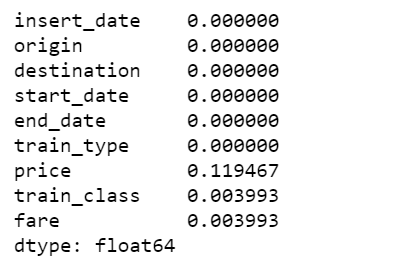
data.isnull().sum()/len(data)
Figure 1
There are 12% of values in price column are missing, I decide to fill them with the mean of the respective fare types. Also fill the other two categorical columns with the most common values.
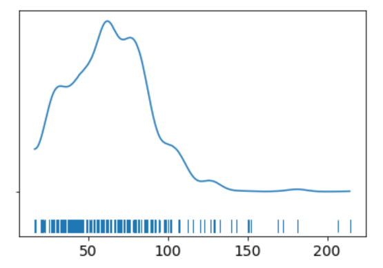
The KDE plot of the rail ticket price shows a Gaussian-like distribution, except for about several dozens of data points that are far away from the mean.
Let’s assume that a Gaussian distribution is a proper description of the rail ticket price. Since we do not know the mean or the standard deviation, we must set priors for both of them. Therefore, a reasonable model could be as follows.
Model
We will perform Gaussian inferences on the ticket price data. Here’s some of the modelling choices that go into this.
We would instantiate the Models in PyMC3 like this:
Model specifications in PyMC3 are wrapped in a with-statement.
Choices of priors:
μ, mean of a population. Normal distribution, very wide. I do not know the possible values of μ, I can set priors reflecting my ignorance. From experience I know that train ticket price can not be lower than 0 or higher than 300, so I set the boundaries of the uniform distribution to be 0 and 300. You may have different experience and set the different boundaries. That is totally fine. And if you have more reliable prior information than I do, please use it!
σ, standard deviation of a population. Can only be positive, therefore use HalfNormal distribution. Again, very wide.
Choices for ticket price likelihood function:
y is an observed variable representing the data that comes from a normal distribution with the parameters μ and σ.
Draw 1000 posterior samples using NUTS sampling.
Using PyMC3, we can write the model as follows:
The y specifies the likelihood. This is the way in which we tell PyMC3 that we want to condition for the unknown on the knows (data).
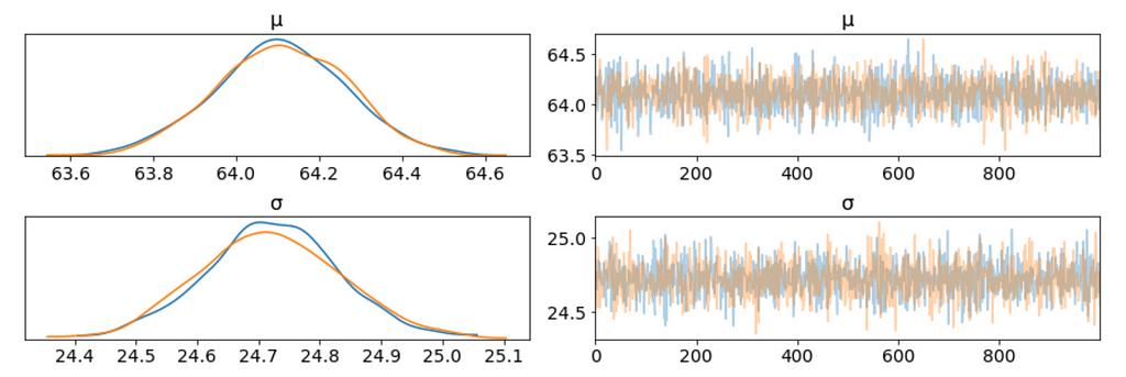
We plot the gaussian model trace. This runs on a Theano graph under the hood.
az.plot_trace(trace_g);
Figure 3
On the left, we have a KDE plot, — for each parameter value on the x-axis we get a probability on the y-axis that tells us how likely that parameter value is.
On the right, we get the individual sampled values at each step during the sampling. From the trace plot, we can visually get the plausible values from the posterior.
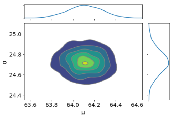
The above plot has one row for each parameter. For this model, the posterior is bi-dimensional, and so the above figure is showing the marginal distributions of each parameter.
There are a couple of things to notice here:
Our sampling chains for the individual parameters (left) seem well converged and stationary (there are no large drifts or other odd patterns).
The maximum posterior estimate of each variable (the peak in the left side distributions) is very close to the true parameters.
I don’t see any correlation between these two parameters. This means we probably do not have collinearityin the model. This is good.
We can also have a detailed summary of the posterior distribution for each parameter.
az.summary(trace_g)
Table 2
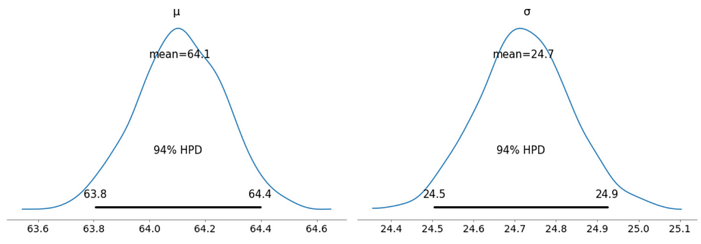
We can also see the above summary visually by generating a plot with the mean and Highest Posterior Density (HPD) of a distribution, and to interpret and report the results of a Bayesian inference.
Every time ArviZ computes and reports a HPD, it will use, by default, a value of 94%.
Please note that HPD intervals are not the same as confidence intervals.
Here we can interpret as such that there is 94% probability the belief is between 63.8 euro and 64.4 euro for the mean ticket price.
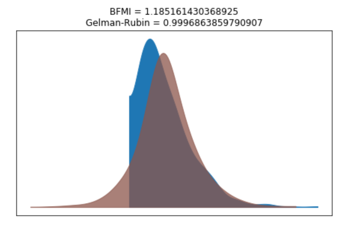
We can verify the convergence of the chains formally using the Gelman Rubin test. Values close to 1.0 mean convergence.
pm.gelman_rubin(trace_g)
bfmi = pm.bfmi(trace_g)
max_gr = max(np.max(gr_stats) for gr_stats in pm.gelman_rubin(trace_g).values())
(pm.energyplot(trace_g, legend=False, figsize=(6, 4)).set_title("BFMI = {}nGelman-Rubin = {}".format(bfmi, max_gr)));
Figure 6
Our model has converged well and the Gelman-Rubin statistic looks fine.
Posterior Predictive Checks
Posterior predictive checks (PPCs) are a great way to validate a model. The idea is to generate data from the model using parameters from draws from the posterior.
Now that we have computed the posterior, we are going to illustrate how to use the simulation results to derive predictions.
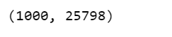
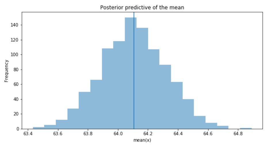
The following function will randomly draw 1000 samples of parameters from the trace. Then, for each sample, it will draw 25798 random numbers from a normal distribution specified by the values of μ and σ in that sample.
Now, ppc contains 1000 generated data sets (containing 25798 samples each), each using a different parameter setting from the posterior.
_, ax = plt.subplots(figsize=(10, 5))
ax.hist([y.mean() for y in ppc['y']], bins=19, alpha=0.5)
ax.axvline(data.price.mean())
ax.set(title='Posterior predictive of the mean', xlabel='mean(x)', ylabel='Frequency');
Figure 7
The inferred mean is very close to the actual rail ticket price mean.
Group Comparison
We may be interested in how price compare under different fare types. We are going to focus on estimating the effect size, that is, quantifying the difference between two fare categories. To compare fare categories, we are going to use the mean of each fare type. Because we are Bayesian, we will work to obtain a posterior distribution of the differences of means between fare categories.
We create three variables:
The price variable, representing the ticket price.
The idx variable, a categorical dummy variable to encode the fare categories with numbers.
And finally the groups variable, with the number of fare categories (6)
The model for the group comparison problem is almost the same as the previous model. the only difference is that μ and σ are going to be vectors instead of scalar variables. This means that for the priors, we pass a shape argument and for the likelihood, we properly index the means and sd variables using the idx variable:
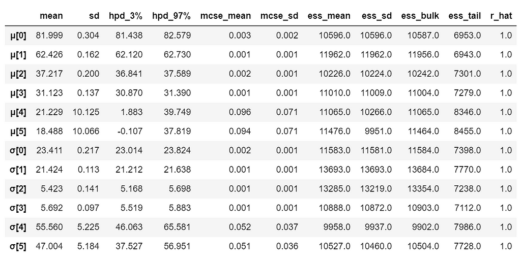
With 6 groups (fare categories), its a little hard to plot trace plot for μ and σ for every group. So, we create a summary table:
It is obvious that there are significant differences between groups (i.e. fare categories) on the mean.
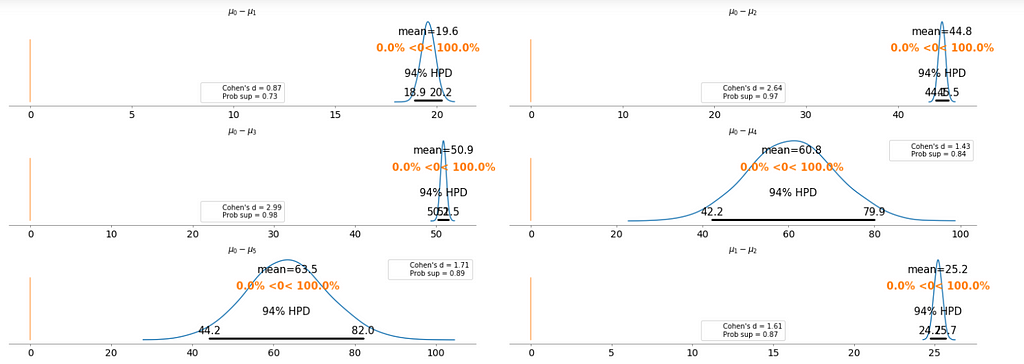
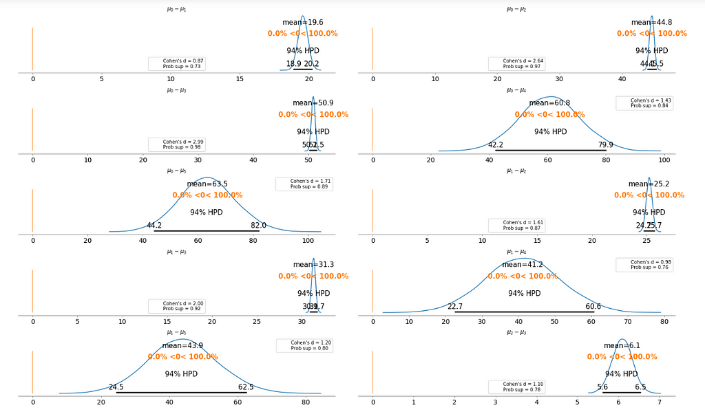
To make it clearer, we plot the difference between each fare category without repeating the comparison.
Cohen’s d is an appropriate effect size for the comparison between two means. Cohen’s d introduces the variability of each group by using their standard deviations.
probability of superiority (ps) is defined as the probability that a data point taken at random from one group has a larger value than one taken at random from another group.
Figure 8
Basically, the above plot tells us that none of the above comparison cases where the 94% HPD includes the reference value of zero. This means for all the examples, we can rule out a difference of zero. The average differences range of 6.1 euro to 63.5 euro are large enough that it can justify for customers to purchase tickets according to different fare categories.
Bayesian Hierarchical Linear Regression
We want to build a model to estimate the rail ticket price of each train type, and, at the same time, estimate the price of all the train types. This type of model is known as a hierarchical model or multilevel model.
Encoding the categorical variable.
The idx variable, a categorical dummy variable to encode the train types with numbers.
And finally the groups variable, with the number of train types (16)
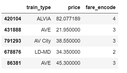
Table 4
The relevant part of the data we will model looks as above. And we are interested in whether different train types affect the ticket price.
Hierarchical Model
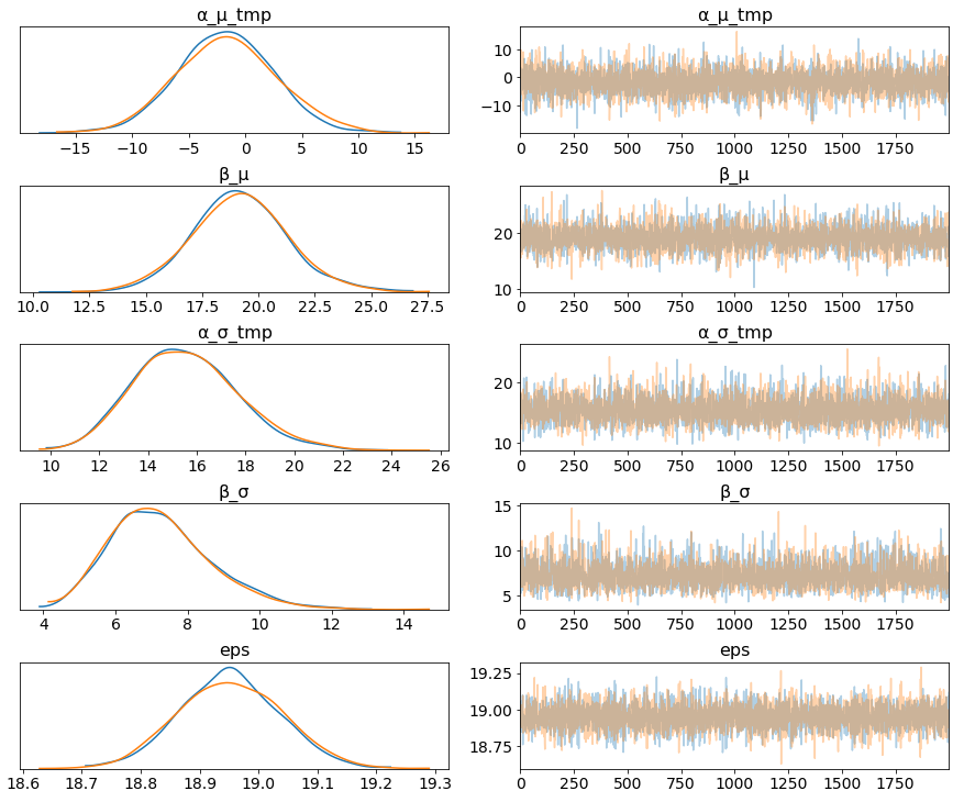
Figure 9
The marginal posteriors in the left column are highly informative, “α_μ_tmp” tells us the group mean price levels, “β_μ” tells us that purchasing fare category “Promo +” increases price significantly compare to fare type “Adulto ida”, and purchasing fare category “Promo” increases price significantly compare to fare type “Promo +”, and so on (no mass under zero).
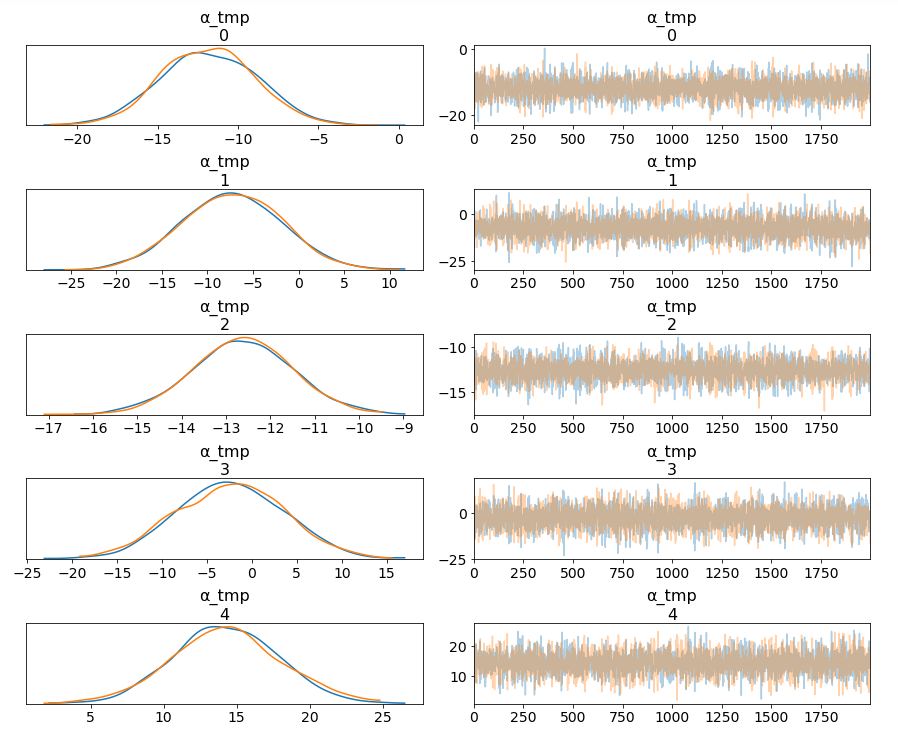
Among 16 train types, we may want to look at how 5 train types compare in terms of the ticket price. We can see by looking at the marginals for “α_tmp” that there is quite some difference in prices between train types; the different widths are related to how much confidence we have in each parameter estimate — the more measurements per train type, the higher our confidence will be.
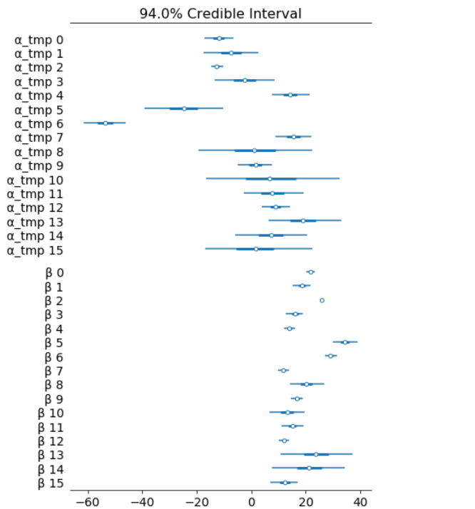
Having uncertainty quantification of some of our estimates is one of the powerful things about Bayesian modelling. We’ve got a Bayesian credible interval for the price of different train types.
The objective of this post is to learn, practice and explain Bayesian, not to produce the best possible results from the data set. Otherwise, we would have gone with XGBoost directly.
Demonstrable understanding of deep learning. Apply state-of-the-art machine learning techniques to real-time industrial sensor data…. From Interaptix Augmented Reality – Wed, 17 Jul 2019 19:35:58 GMT – View all Toronto, ON jobs
Climate researchers look into the future to project how much the planet will warm in coming decades — but they often rely on decades-old software to conduct their analyses.
This legacy software architecture is difficult to update with new methodologies that have emerged in recent years. So a consortium of researchers is starting from scratch, writing a new climate model that leverages AI, new software tools and NVIDIA GPUs.
Scientists from Caltech, MIT, the Naval Postgraduate School and NASA’s Jet Propulsion Laboratory are part of the initiative, named the Climate Modeling Alliance — or CliMA.
“Computing has advanced quite a bit since the ‘60s,” said Raffaele Ferrari, oceanography professor at MIT and principal investigator on the project. “We know much more than we did at that time, but a lot was hard-coded into climate models when they were first developed.”
Building a new climate model from the ground up allows climate researchers to better account for small-scale environmental features, including cloud cover, rainfall, sea ice and ocean turbulence.
These variables are too geographically miniscule to be precisely captured in climate models, but can be better approximated using AI. Incorporating the AI’s projections into the new climate model could reduce uncertainties by half compared to existing models.
The team is developing the new model using Julia, an MIT-developed programming language that was designed for parallelism and distributed computation, allowing the scientists to accelerate their climate model calculations using NVIDIA V100 Tensor Core GPUs onsite and on Google Cloud.
As the project progresses, the researchers plan to use supercomputers like the GPU-powered Summit system at Oak Ridge National Labs as well as commercial cloud resources to run the new climate model — which they hope to have running within the next five years.
AI Turns the Tide
Climate scientists use physics and thermodynamics equations to calculate the evolution of environmental variables like air temperature, sea level and rainfall. But it’s incredibly computationally intensive to run these calculations for the entire planet. So in existing models, researchers divide the globe into a grid of 100-square-kilometer sections.
They calculate every 100 km block independently, using mathematical approximations for smaller features like turbulent eddies in the ocean and low-lying clouds in the sky — which can measure less than one kilometer across. As a result, when stringing the grid back together into a global model, there’s a margin of uncertainty introduced in the output.
Small uncertainties can make a significant difference, especially when climate scientists are estimating for policymakers how many years it will take for average global temperature to rise by more than two degrees Celcius. Due to the current levels of uncertainty, researchers project that, with current emission levels, this threshold could be crossed as soon as 2040 — or as late as 2100.
“That’s a huge margin of uncertainty,” said Ferrari. “Anything to reduce that margin can provide a societal benefit estimated in trillions of dollars. If one knows better the likelihood of changes in rainfall patterns, for example, then everyone from civil engineers to farmers can decide what infrastructure and practices they may need to plan for.”
A Deep Dive into Ocean Data
The MIT researchers are focusing on building the ocean elements of CliMA’s new climate model. Covering around 70 percent of the planet’s surface, oceans are a major heat and carbon dioxide reservoir. To make ocean-related climate projections, scientists look at such variables as water temperature, salinity and velocity of ocean currents.
One such dynamic is turbulent streams of water that flow around in the ocean like “a lot of little storms,” Ferrari said. “If you don’t account for all that swirling motion, you strongly underestimate how the ocean is absorbing heat and carbon.”
Using GPUs, researchers can narrow the resolution of their high-resolution simulations from 100 square kilometers down to one square kilometer, dramatically reducing uncertainties. But these simulations are too expensive to directly incorporate into a climate model that looks decades into the future.
That’s where an AI model that learns from fine-resolution ocean and cloud simulations can help.
“Our goal is to run thousands of high-resolution simulations, one for each 100-by-100 kilometer block, that will resolve the small-scale physics presently not captured by climate models,” said Chris Hill, principal research engineer at MIT’s earth, atmospheric and planetary sciences department.
These high-resolution simulations produce abundant synthetic data. That data can be combined with sparser real-world measurements, creating a robust training dataset for an AI model that estimates the impact of small-scale physics like ocean turbulence and cloud patterns on large-scale climate variables.
CliMA researchers can then plug these AI tools into the new climate model software, improving the accuracy of long-term projections.
“We’re betting a lot on GPU technology to provide a boost in compute performance,” Hill said.
MIT hosted in June a weeklong GPU hackathon, where developers — including Hill’s team as well as research groups from other universities — used the CUDA parallel computing platform and the Julia programming language for projects such as ocean modeling, plasma fusion and astrophysics.
The growth of artificial intelligence could create 58 million net new jobs in the next few years, states the World Economic Forum [1]. Yet, according to the Tencent Research Institute, it’s estimated that currently there are 300,000 AI engineers worldwide, but millions are needed [2]. As you can tell, there is a unique and immediate opportunity to develop creative experiences and introduce you—no matter what your developer skill levels are—to essential ML concepts. These experiences in fields of ML like deep learning, reinforcement learning, and so on, will expand your skills and help close the talent gap.
To help you advance your AI/ML capabilities with hands-on and fun ML learning experiences, I am thrilled to announce the AWS DeepRacer Scholarship Challenge.
What is AWS DeepRacer?
In November 2018, Jeff Barr announced the launch of AWS DeepRacer on the AWS News Blog as a new way to learn ML. With AWS DeepRacer, you have an opportunity to get hands-on with a fully autonomous 1/18th-scale race car driven by reinforcement learning, a 3D racing simulator, and a global racing league.
What is the AWS DeepRacer Scholarship Challenge?
AWS and Udacity are collaborating to educate developers of all skill levels on ML concepts. Those skills are reinforced by putting them to the test through the world’s first autonomous racing league—the AWS DeepRacer League.
How does the AWS DeepRacer Scholarship Challenge work?
The program begins August 1, 2019 and runs through October 31, 2019. You can join the scholarship community at any point during these three months and immediately enroll in Udacity’s specialized AWS DeepRacer course. Register now to be in pole position for the start of the race.
After enrollment, you go through the AWS DeepRacer course, which consists of short, step-by-step modules (90 minutes in total). The modules prepare you to create, train, and fine-tune a reinforcement learning model in the AWS DeepRacer 3D racing simulator. Throughout the program and during each race, you have access to a custom scholarship student community to get pro tips from experts and exchange ideas with your classmates.
Each month, you can pit your skills against others in virtual races in the AWS DeepRacer console. Students compete for top spots in each month’s unique race course. Students that record the top lap times in August, September, and October 2019 qualify for one of 200 full scholarships to the Udacity Machine Learning Engineer nanodegree program, sponsored by Udacity.
Tara Shankar Jana is a Senior Product Marketing Manager for AWS Machine Learning. Currently he is working on building unique and scalable educational offerings for the aspiring ML developer communities- to help them expand their skills on ML. Outside of work he loves reading books, travelling and spending time with his family.





 Tara Shankar Jana is a Senior Product Marketing Manager for AWS Machine Learning. Currently he is working on building unique and scalable educational offerings for the aspiring ML developer communities- to help them expand their skills on ML. Outside of work he loves reading books, travelling and spending time with his family.