Category: Global
Microsoft launches business school focused on AI strategy, culture and responsibility
In recent years, some of the world’s fastest growing companies have deployed artificial intelligence to solve specific business problems. In fact, according to new market research from Microsoft on how AI will change leadership, these high-growth companies are more than twice as likely to be actively implementing AI as lower-growth companies.
What’s more, high-growth companies are further along in their AI deployments, with about half planning to use more AI in the coming year to improve decision making compared to about a third of lower growth companies. Still, less than two in 10 of even high-growth companies are integrating AI across their operations, the research found.
“There is a gap between what people want to do and the reality of what is going on in their organizations today, and the reality of whether their organization is ready,” said Mitra Azizirad, corporate vice president for AI marketing at Microsoft in Redmond, Washington.
“Developing a strategy for AI extends beyond the business issues,” she explained. “It goes all the way to the leadership, behaviors and capabilities required to instill an AI-ready culture in your organization.”
On the road to developing a strategy, executives and other business leaders are often stalled by questions about how and where to begin implementing AI across their companies; the cultural changes that AI requires companies to make; and how to build and use AI in ways that are responsible, protect privacy and security, and comply with government rules and regulations.
Today, Azizirad and her team are launching Microsoft’s AI Business School to help business leaders navigate these questions. The free, online course is a master class series that aims to empower business leaders to lead with confidence in the age of AI.
Focus on strategy, culture and responsibility
AI Business School course materials include brief written case studies and guides, plus videos of lectures, perspectives and talks that busy executives can access in small doses when they have time. A series of short introductory videos provide an overview of the AI technologies driving change across industries, but the bulk of the content focuses on managing the impact of AI on company strategy, culture and responsibility.
“This school is a deep dive into how you develop a strategy and identify blockers before they happen in the implementation of AI in your organization,” said Azizirad.
The business school complements other AI learning initiatives across Microsoft, including the developer-focused AI School and the Microsoft Professional Program for Artificial Intelligence, which provides job-ready skills and real-world experience to engineers and others looking to improve their skills in AI and data science.
Unlike these other initiatives, AI Business School is non-technical and designed to get executives ready to lead their organizations on a journey of AI transformation, according to Azizirad.
Nick McQuire, an analyst who covers artificial intelligence for CCS Insight, said more than 50 percent of the companies his firm has surveyed are already either researching, trialing or implementing specific projects with AI and machine learning, but very few are using AI across their organization and identifying business opportunities and problems that AI can address.
“That’s because there’s limited understanding in the business community about what AI is, what it can do and, ultimately, what are the applications,” he said. “Microsoft is trying to fill that gap.”
 Mitra Azizirad, corporate vice president for AI marketing. Photo by Microsoft.
Teaching by example
INSEAD, a graduate business school with campuses in Europe, Asia and the Middle East, partnered with Microsoft to build the AI Business School’s strategy module, which includes case studies about companies across many industries that have successfully transformed their businesses with AI.
For example, a case study on Jabil describes how one of the world’s largest manufacturing solutions providers was able to reduce overhead costs and increase production line quality by using AI to check electronic parts as they are manufactured, freeing up employees to focus on value added activities that machines are unable to do.
“There is still a lot of work that has got to have the human capital piece in it, especially if it is not something that lends itself to standardized processes,” explained Gary Cantrell, senior vice president and chief information officer for Jabil.
A key to implementing AI, Cantrell added, was the leadership team’s focus on clearly communicating to employees the company’s strategy around AI – to eliminate routine, repetitive activities in order to free them up to focus on activities that cannot be automated.
“If they are guessing or they are speculating, it is undoubtedly going to become counterproductive at some point,” he said. “So, the better job you do at keeping the team glued together with where you are going, the better the adoption will be and the faster it will be.”
Prepping an AI-ready culture
The culture and responsibility modules of AI Business School also place a core focus on data. After all, companies that successfully embrace AI need to openly share data across departments and business functions, explained Azizirad, and make sure all employees can participate in the development and implementation of data-driven AI applications.
“You need to start out with an open approach to how the data of an organization is going to be used, which is the foundation of AI, to get the results that you are banking on,” she said, adding that successful leaders foster an inclusive approach to AI that brings different roles together and breaks down data silos.
To illustrate the point, the Microsoft AI Business School surfaces a case study from Microsoft’s marketing team, which wanted to use AI to better score leads for the sales team to pursue. To build the solution, marketing employees partnered with data scientists to create machine learning models that weigh thousands of variables to score leads. The collaboration brought together marketing employees’ knowledge on lead quality with the machine learning expertise of data scientists.
“In the case of AI and in the case of culture, the people closest to the business problem you are trying to solve really need to be involved,” said Azizirad, adding that the sales team is embracing the lead-scoring model because they trust it will produce high-quality leads.
AI and responsibility
Building trust also comes from developing and deploying AI systems in a responsible manner, an area that Microsoft’s market research has found resonates with business leaders. Among high-growth companies, the research found, the more leaders know about AI, the more they recognize that they need to make sure the AI is deployed responsibly.
The AI Business School module on the implications of responsible AI showcases Microsoft’s own work in this area. Course materials include real-world examples in which leaders at Microsoft learned lessons such as the need to safeguard AI systems against malicious attacks and the need for systems to detect bias in datasets used to train models.
“Over time, as companies become operationally dependent on these machine learning algorithms and models that they built, there’s going to be much more focus on governance,” said McQuire, the CCS Insight analyst.
Related:
- Check out AI Business School
- Read: Leaders look to embrace AI, and high-growth companies are seeing the benefits
- Read: Aiming to fill skills gap in AI, Microsoft makes training courses available to the public
- Read: Microsoft Launches Free AI Business School for Execs
John Roach writes about Microsoft research and innovation. Follow him on Twitter.
The post Microsoft launches business school focused on AI strategy, culture and responsibility appeared first on The AI Blog.
Real-Time AR Self-Expression with Machine Learning
Augmented reality (AR) helps you do more with what you see by overlaying digital content and information on top of the physical world. For example, AR features coming to Google Maps will let you find your way with directions overlaid on top of your real world. With Playground – a creative mode in the Pixel camera — you can use AR to see the world differently. And with the latest release of YouTube Stories and ARCore‘s new Augmented Faces API you can add objects like animated masks, glasses, 3D hats and more to your own selfies!
One of the key challenges in making these AR features possible is proper anchoring of the virtual content to the real world; a process that requires a unique set of perceptive technologies able to track the highly dynamic surface geometry across every smile, frown or smirk.
 |
| Our 3D mesh and some of the effects it enables |
To make all this possible, we employ machine learning (ML) to infer approximate 3D surface geometry to enable visual effects, requiring only a single camera input without the need for a dedicated depth sensor. This approach provides the use of AR effects at realtime speeds, using TensorFlow Lite for mobile CPU inference or its new mobile GPU functionality where available. This technology is the same as what powers YouTube Stories’ new creator effects, and is also available to the broader developer community via the latest ARCore SDK release and the ML Kit Face Contour Detection API.
An ML Pipeline for Selfie AR
Our ML pipeline consists of two real-time deep neural network models that work together: A detector that operates on the full image and computes face locations, and a generic 3D mesh model that operates on those locations and predicts the approximate surface geometry via regression. Having the face accurately cropped drastically reduces the need for common data augmentations like affine transformations consisting of rotations, translation and scale changes. Instead it allows the network to dedicate most of its capacity towards coordinate prediction accuracy, which is critical to achieve proper anchoring of the virtual content.
Once the location of interest is cropped, the mesh network is only applied to a single frame at a time, using a windowed smoothing in order to reduce noise when the face is static while avoiding lagging during significant movement.
 |
| Our 3D mesh in action |
For our 3D mesh we employed transfer learning and trained a network with several objectives: the network simultaneously predicts 3D mesh coordinates on synthetic, rendered data and 2D semantic contours on annotated, real world data similar to those MLKit provides. The resulting network provided us with reasonable 3D mesh predictions not just on synthetic but also on real world data. All models are trained on data sourced from a geographically diverse dataset and subsequently tested on a balanced, diverse testset for qualitative and quantitative performance.
The 3D mesh network receives as input a cropped video frame. It doesn’t rely on additional depth input, so it can also be applied to pre-recorded videos. The model outputs the positions of the 3D points, as well as the probability of a face being present and reasonably aligned in the input. A common alternative approach is to predict a 2D heatmap for each landmark, but it is not amenable to depth prediction and has high computational costs for so many points.
We further improve the accuracy and robustness of our model by iteratively bootstrapping and refining predictions. That way we can grow our dataset to increasingly challenging cases, such as grimaces, oblique angle and occlusions. Dataset augmentation techniques also expanded the available ground truth data, developing model resilience to artifacts like camera imperfections or extreme lighting conditions.
 |
| Dataset expansion and improvement pipeline |
Hardware-tailored Inference
We use TensorFlow Lite for on-device neural network inference. The newly introduced GPU back-end acceleration boosts performance where available, and significantly lowers the power consumption. Furthermore, to cover a wide range of consumer hardware, we designed a variety of model architectures with different performance and efficiency characteristics. The most important differences of the lighter networks are the residual block layout and the accepted input resolution (128×128 pixels in the lightest model vs. 256×256 in the most complex). We also vary the number of layers and the subsampling rate (how fast the input resolution decreases with network depth).
 |
| Inference time per frame: CPU vs. GPU |
The result of these optimizations is a substantial speedup from using lighter models, with minimal degradation in AR effect quality.
 |
| Comparison of the most complex (left) and the lightest models (right). Temporal consistency as well as lip and eye tracking is slightly degraded on light models. |
The end result of these efforts empowers a user experience with convincing, realistic selfie AR effects in YouTube, ARCore, and other clients by:
- Simulating light reflections via environmental mapping for realistic rendering of glasses
- Natural lighting by casting virtual object shadows onto the face mesh
- Modelling face occlusions to hide virtual object parts behind a face, e.g. virtual glasses, as shown below.
 |
| YouTube Stories includes Creator Effects like realistic virtual glasses, based on our 3D mesh |
In addition, we achieve highly realistic makeup effects by:
- Modelling Specular reflections applied on lips and
- Face painting by using luminance-aware material
 |
| Case study comparing real make-up against our AR make-up on 5 subjects under different lighting conditions. |
We are excited to share this new technology with creators, users and developers alike, who can use this new technology immediately by downloading the latest ARCore SDK. In the future we plan to broaden this technology to more Google products.
Acknowledgements
We would like to thank Yury Kartynnik, Valentin Bazarevsky, Andrey Vakunov, Siargey Pisarchyk, Andrei Tkachenka, and Matthias Grundmann for collaboration on developing the current mesh technology; Nick Dufour, Avneesh Sud and Chris Bregler for an earlier version of the technology based on parametric models; Kanstantsin Sokal, Matsvei Zhdanovich, Gregory Karpiak, Alexander Kanaukou, Suril Shah, Buck Bourdon, Camillo Lugaresi, Siarhei Kazakou and Igor Kibalchich for building the ML pipeline to drive impressive effects; Aleksandra Volf and the annotation team for their diligence and dedication to perfection; Andrei Kulik, Juhyun Lee, Raman Sarokin, Ekaterina Ignasheva, Nikolay Chirkov, and Yury Pisarchyk for careful benchmarking and insights on mobile GPU-centric network architecture optimizations.

Is drought on the horizon? Researchers turn to AI in a bid to improve forecasts
As winter drags on, some people wonder whether to pack shorts for a late-March escape to Florida, while others eye April temperature trends in anticipation of sowing crops. Water managers in the western U.S. check for the possibility of early-spring storms to top off mountain snowpack that is crucial for irrigation, hydropower and salmon in the summer months.
Unfortunately, forecasts for this timeframe — roughly two to six weeks out — are a crapshoot, noted Lester Mackey, a statistical machine learning researcher at Microsoft’s New England research lab in Cambridge, Massachusetts. Mackey is bringing his expertise in artificial intelligence to the table in a bid to increase the odds of accurate and reliable forecasts.
“The subseasonal regime is where forecasts could use the most help,” he said.
Mackey knew little about weather and climate forecasting until Judah Cohen, a climatologist at Atmospheric and Environmental Research, a Verisk business that consults about climate risk in Lexington, Massachusetts, reached out to him for help using machine learning techniques to tease out repeating weather and climate patterns from mountains of historical data as a way to improve subseasonal and seasonal forecast models.
The preliminary machine learning based forecast models that Mackey, Cohen and their colleagues developed outperformed the standard models used by U.S. government agencies to generate subseasonal forecasts of temperature and precipitation two to four weeks out and four to six weeks out in a competition sponsored by the U.S. Bureau of Reclamation.
Mackey’s team recently secured funding from Microsoft’s AI for Earth initiative to improve and refine its technique with an eye toward advancing the technology for the social good.
“Lester is working on this because it is a hard problem in machine learning, not because it is a hard problem in weather forecasting,” noted Lucas Joppa, Microsoft’s chief environmental officer who runs the AI for Earth program, as he explained why his group is helping fund the research. “It just so happens that the techniques he is interested in exploring have huge applicability in weather forecasting, which happens to have huge applicability in broader societal and economic domains.”
 Photo by Getty Images.
AI on the brain
Mackey said current weather models perform well up to about seven days in advance, and climate forecast models get more reliable as the time horizon extends from seasons to decades. Subseasonal forecasts are a middle ground, relying on a mix of variables that impact short-term weather such as daily temperature and wind and seasonal factors such as the state of El Niño and the extent of sea ice in the Arctic.
Cohen contacted Mackey out of a belief that machine learning, the arm of AI that encompasses recognizing patterns in statistical data to make predictions, could help improve his method of generating subseasonal forecasts by gleaning insights from troves of historical weather and climate data.
“I am basically doing something like machine learned pattern recognition in my head,” explained Cohen, noting that weather patterns repeat throughout the seasons and from year to year and that therefore pattern recognition can and should inform longer-term forecasts. “I thought maybe I can improve on what I am doing in my head with some of the machine learning techniques that are out there.”
Using patterns in historical weather data to predict the future was standard practice in weather and climate forecast generation until the 1980s. That’s when physical models of how the atmosphere and oceans evolve began to dominate the industry. These models have grown in popularity and sophistication with the exponential rise in computing power.
“Today, all of the major climate centers employ massive supercomputers to simulate the atmosphere and oceans,” said Mackey. “The forecasts have improved substantially over time, but they make relatively little use of historical data. Instead, they ingest today’s weather conditions and then push forward their differential equations.”
 Photo by Getty Images.
Forecast competition
As Mackey and Cohen were discussing a research collaboration, Cohen received notice of a competition sponsored by the U.S. Bureau of Reclamation to improve subseasonal forecasts of temperature and precipitation in the western U.S. The government agency is interested in improved subseasonal forecasts to better prepare water managers for shifts in hydrologic regimes, including the onset of drought and wet weather extremes.
“I said, ‘Hey, what do you think about trying to enter this competition as a way to motivate us, to make some progress,’” recalled Cohen.
Mackey, who was an assistant professor of statistics at Stanford University in California prior to joining Microsoft’s research organization and remains an adjunct professor at the university, invited two graduate students to participate on the project. “None of us had experience doing work in this area and we thought this would be a great way to get our feet wet,” he said.
Over the course of the 13-month competition, the researchers experimented with two types of machine learning approaches. One combed through a kitchen sink of data containing everything from historical temperature and precipitation records to data on sea ice concentration and the state of El Niño as well as an ensemble of physical forecast models. The other approach focused only on historical data for temperature when forecasting temperature or precipitation when forecasting precipitation.
“We were making forecasts every two weeks and between those forecasts we were acquiring new data, processing it, building some of the infrastructure for testing out new methods, developing methods and evaluating them,” Mackey explained. “And then every two weeks we had to stop what we were doing and just make a forecast and repeat.”
Toward the end of the competition, Mackey’s team discovered that an ensemble of both machine learning approaches performed better than either alone.
Final results of the competition were announced today. Mackey, Cohen and their colleagues captured first place in forecasting average temperature three to four weeks in advance and second place in forecasting total precipitation five and six weeks out.
 Photo by Getty Images.
Forecast for the future
After the competition, the collaborators combined their ensemble of machine learning approaches with the standard models used by U.S. government agencies to generate subseasonal forecasts and found that the combined models improved the accuracy of the operational forecast by between 37 and 53 percent for temperature and 128 and 154 percent for precipitation. These results are reported in a paper the team posted on arXiv.org.
“I think we will continue to see these types of approaches be further refined and increase in the breadth of their use within the field of forecasting,” said Kenneth Nowak, water availability research coordinator with the U.S. Bureau of Reclamation, who organized the forecast rodeo. He added that government agencies will “look for opportunities to leverage” machine learning in future generations of operational forecast models.
Microsoft’s AI for Earth program is providing funding to Mackey and colleagues to hire an intern to expand and refine their machine learning based forecasting technique. The collaborators also hope that other machine learning researchers will be drawn to the challenge of cracking the code to accurate and reliable subseasonal forecasts. To encourage these efforts, they have made available to the public the dataset they created to train their models.
Cohen, who kicked off the collaboration with Mackey out of a curiosity about the potential impact of AI on subseasonal to seasonal climate forecasts, said, “I see the benefit of machine learning, absolutely. This is not the end; more like the beginning. There is a lot more that we can do to increase its applicability.”
Related:
- Learn more about the U.S. Subseasonal Climate Forecast Rodeo
- Read the paper: Improving Subseasonal Forecasting in the Western U.S. with Machine Learning
- Access the SubseasonalRodeo Dataset
- Lester Mackey is a statistical machine learning researcher at Microsoft’s New England research lab.
- Judah Cohen is the head of seasonal forecasting at Atmospheric and Environmental Research.
- Lucas Joppa is Microsoft’s chief environmental officer and leads the AI for Earth initiative.
John Roach writes about Microsoft research and innovation. Follow him on Twitter.
The post Is drought on the horizon? Researchers turn to AI in a bid to improve forecasts appeared first on The AI Blog.
RNN-Based Handwriting Recognition in Gboard
In 2015 we launched Google Handwriting Input, which enabled users to handwrite text on their Android mobile device as an additional input method for any Android app. In our initial launch, we managed to support 82 languages from French to Gaelic, Chinese to Malayalam. In order to provide a more seamless user experience and remove the need for switching input methods, last year we added support for handwriting recognition in more than 100 languages to Gboard for Android, Google’s keyboard for mobile devices.
Since then, progress in machine learning has enabled new model architectures and training methodologies, allowing us to revise our initial approach (which relied on hand-designed heuristics to cut the handwritten input into single characters) and instead build a single machine learning model that operates on the whole input and reduces error rates substantially compared to the old version. We launched those new models for all latin-script based languages in Gboard at the beginning of the year, and have published the paper “Fast Multi-language LSTM-based Online Handwriting Recognition” that explains in more detail the research behind this release. In this post, we give a high-level overview of that work.

Touch Points, Bézier Curves and Recurrent Neural Networks
The starting point for any online handwriting recognizer are the touch points. The drawn input is represented as a sequence of strokes and each of those strokes in turn is a sequence of points each with a timestamp attached. Since Gboard is used on a wide variety of devices and screen resolutions our first step is to normalize the touch-point coordinates. Then, in order to capture the shape of the data accurately, we convert the sequence of points into a sequence of cubic Bézier curves to use as inputs to a recurrent neural network (RNN) that is trained to accurately identify the character being written (more on that step below). While Bézier curves have a long tradition of use in handwriting recognition, using them as inputs is novel, and allows us to provide a consistent representation of the input across devices with different sampling rates and accuracies. This approach differs significantly from our previous models which used a so-called segment-and-decode approach, which involved creating several hypotheses of how to decompose the strokes into characters (segment) and then finding the most likely sequence of characters from this decomposition (decode).
Another benefit of this method is that the sequence of Bézier curves is more compact than the underlying sequence of input points, which makes it easier for the model to pick up temporal dependencies along the input — Each curve is represented by a polynomial defined by start and end-points as well as two additional control points, determining the shape of the curve. We use an iterative procedure which minimizes the squared distances (in x, y and time) between the normalized input coordinates and the curve in order to find a sequence of cubic Bézier curves that represent the input accurately. The figure below shows an example of the curve fitting process. The handwritten user-input can be seen in black. It consists of 186 touch points and is clearly meant to be the word go. In yellow, blue, pink and green we see its representation through a sequence of four cubic Bézier curves for the letter g (with their two control points each), and correspondingly orange, turquoise and white represent the three curves interpolating the letter o.

Character Decoding
The sequence of curves represents the input, but we still need to translate the sequence of input curves to the actual written characters. For that we use a multi-layer RNN to process the sequence of curves and produce an output decoding matrix with a probability distribution over all possible letters for each input curve, denoting what letter is being written as part of that curve.
We experimented with multiple types of RNNs, and finally settled on using a bidirectional version of quasi-recurrent neural networks (QRNN). QRNNs alternate between convolutional and recurrent layers, giving it the theoretical potential for efficient parallelization, and provide a good predictive performance while keeping the number of weights comparably small. The number of weights is directly related to the size of the model that needs to be downloaded, so the smaller the better.
In order to “decode” the curves, the recurrent neural network produces a matrix, where each column corresponds to one input curve, and each row corresponds to a letter in the alphabet. The column for a specific curve can be seen as a probability distribution over all the letters of the alphabet. However, each letter can consist of multiple curves (the g and o above, for instance, consist of four and three curves, respectively). This mismatch between the length of the output sequence from the recurrent neural network (which always matches the number of bezier curves) and the actual number of characters the input is supposed to represent is addressed by adding a special blank symbol to indicate no output for a particular curve, as in the Connectionist Temporal Classification (CTC) algorithm. We use a Finite State Machine Decoder to combine the outputs of the Neural Network with a character-based language model encoded as a weighted finite-state acceptor. Character sequences that are common in a language (such as “sch” in German) receive bonuses and are more likely to be output, whereas uncommon sequences are penalized. The process is visualized below.

The sequence of touch points (color-coded by the curve segments as in the previous figure) is converted to a much shorter sequence of Bezier coefficients (seven, in our example), each of which corresponds to a single curve. The QRNN-based recognizer converts the sequence of curves into a sequence of character probabilities of the same length, shown in the decoder matrix with the rows corresponding to the letters “a” to “z” and the blank symbol, where the brightness of an entry corresponds to its relative probability. Going through the decoder matrix left to right, we see mostly blanks, and bright points for the characters “g” and “o”, resulting in the text output “go”.
Despite being significantly simpler, our new character recognition models not only make 20%-40% fewer mistakes than the old ones, they are also much faster. However, all this still needs to be performed on-device!
Making it Work, On-device
In order to provide the best user-experience, accurate recognition models are not enough — they also need to be fast. To achieve the lowest latency possible in Gboard, we convert our recognition models (trained in TensorFlow) to TensorFlow Lite models. This involves quantizing all our weights during model training such that instead of using four bytes per weight we only use one, which leads to smaller models as well as lower inference times. Moreover, TensorFlow Lite allows us to reduce the APK size compared to using a full TensorFlow implementation, because it is optimized for small binary size by only including the parts which are required for inference.
More to Come
We will continue to push the envelope beyond improving the latin-script language recognizers. The Handwriting Team is already hard at work launching new models for all our supported handwriting languages in Gboard.
Acknowledgements
We would like to thank everybody who contributed to improving the handwriting experience in Gboard. In particular, Jatin Matani from the Gboard team, David Rybach from the Speech & Language Algorithms Team, Prabhu Kaliamoorthi from the Expander Team, Pete Warden from the TensorFlow Lite team, as well as Henry Rowley, Li-Lun Wang, Mircea Trăichioiu, Philippe Gervais, and Thomas Deselaers from the Handwriting Team.
Model serving with Amazon Elastic Inference
Amazon Elastic Inference (EI) is a service that allows you to attach low-cost GPU-powered acceleration to Amazon EC2 and Amazon SageMaker instances. EI reduces the cost of running deep learning inference by up to 75%. Model Server for Apache MXNet (MMS) enables deployment of MXNet- and ONNX-based models for inference at scale. In this blog post, we’ll explore using MMS running on a general purpose EC2 instance with an Elastic Inference Accelerator (EIA) attached.
What is Model Server for Apache MXNet (MMS)?
MMS is an open-source model serving framework designed to simplify the task of serving deep learning models for inference at scale. After training deep learning models using Apache MXNet, MMS makes it easy to deploy the trained model for inference at scale in a production environment. The following architectural diagram shows a standard MMS scalable architecture.

What is Amazon Elastic Inference?
In deep learning applications, inference drives as much as 90 percent of the compute costs of the application. Accelerated GPU instances are oversized for inference because inference happens on a single input in real time that consumes only a small amount of GPU compute. GPU compute capacity usage might not be 100 percent even at peak load, which is wasteful and costly.
EI allows you to attach just the right amount of GPU-powered inference acceleration to any EC2 or Amazon SageMaker instance and save up to 75 percent. With EI, you can now choose the instance type that is best suited to the overall CPU and memory needs of your application, and then you can separately configure the amount of inference acceleration that you need to use resources efficiently and to reduce costs.
Setting up Amazon Elastic Inference with EC2
Starting up an EC2 instance with an attached EI accelerator requires some pre-configuration steps to setup your AWS account. Then, we can launch an instance with an accelerator by following the instructions in the Elastic Inference documentation. Here we’ll use a plain Ubuntu Amazon Machine Image (AMI), and configure it for our needs.
Serving ResNet-152 model with Elastic Inference
After launching an EC2 instance with an EI accelerator, we install MMS and the EI enabled version of MXNet.
Next, let’s start MMS with a ResNet-152 model-archive that is already configured for EI. To build your own model-archive with EIA support refer to Custom Service and Model Serving with Elastic Inference documentation. We configure MMS using a curl command to set the number of workers to 1, and to use synchronous creation of workers.
Notice that we set min_worker=1 in the previous curl command to configure MMS. This is important for MMS on EI because inference calls to the EI accelerator are sequential, so we don’t gain much benefit from using more than one worker. Now the model is ready for some inference requests. To classify an image of a kitten, execute the following commands:
This yields the following prediction results:
You can see that ResNet-152 identified the tabby cat using Elastic Inference hosted with MMS.
Cost and performance benefits of serving with Elastic Inference
In model serving, performance is measured in terms of throughput (number of inferences per second) and latency (time for each inference). For CPU or GPU instances, the best latency is achieved with a single worker, but higher throughput is achieved by using one worker for each vCPU or GPU. We started with an m5.large instance and evaluated both throughput and latency optimized configurations. We achieved a throughput of 4.5 requests per second, and 244ms latency. The cost efficiency of this configuration for 100,000 requests is $0.59. Compare this to the throughput of 41.42 on a p3.2xlarge, 23ms latency, and cost efficiency of $2.05. This can be expensive for production use cases. So, let’s look at how Amazon Elastic Inference can help.
EI accelerators are currently available in three sizes: eia1.medium, eia1.large, and eia1.xlarge. Each has from 1 to 4 GB of memory and from 8 to 32 TFLOPS of compute.
We evaluated performance of this model with an eia1.medium accelerator and observed that larger instance sizes didn’t materially improve latency performance. Next, we tested the m5.large with different EI accelerator sizes. Inference calls with an eia1.large accelerator had lower latency than an eia1.medium, but were not more cost efficient. We use eia1.medium since it provides a good balance between performance and cost for the ResNet-152 model use case.
When optimizing for throughout, the m5.large + eia1.medium instance is 46 percent as fast a regular p3.2xlarge but is 84 percent more cost efficient. It is also 30 percent more cost efficient than a c5.xlarge, while also delivering 1.9x the throughput. The m5.large + eia1.medium provides 4.2x more throughput than just the m5.large alone, with 45 percent better cost efficiency. The following figure shows results when optimizing for maximum throughput.

When optimizing for latency, the m5.large + eia1.medium instance is 43 percent more cost efficient than a c5.xlarge instance, while having 2.4x lower latency. Compared to the m5.large alone, adding an eia1.medium improves cost efficiency by 44 percent with 4.4x better latency. The p3.2xlarge instance has 2.3x lower latency but costs 5.6x more than an m5.large + eia1.medium. The following figure shows results when optimizing for minimum latency.

Conclusion
To recap, in this blog post we showed that Elastic Inference provides the best cost efficiency for running inference at scale while optimizing for latency or throughput.
Learn more about MMS and contribute
Using Elastic Inference is one among many possibilities of hosting models with MMS. To learn more about MMS, start with our examples and documentation in the repository’s model zoo and documentation folder.
We welcome community participation including questions, requests, and contributions, as we continue to improve MMS. If you are using MMS already, we welcome your feedback via the repository’s GitHub issues. Head over to awslabs/mxnet-model-server to get started!
Appendix
The following table shows the specific configuration settings we used, and raw results we presented in this post.
Table 1: Raw Performance and Cost Results for ResNet-152.
| Instance Type | Optimized for | # of workers * | # of OMP threads ** | Hourly cost | Cost Efficiency | Latency (ms) | Throughput (requests/sec) |
| m5.large | Throughput | 2 | 1 | $ 0.10 | $ 0.59 | 444 | 4.50 |
| m5.large | Latency | 1 | 1 | $ 0.10 | $ 0.65 | 244 | 4.08 |
| m5.large + eia.medium | Both | 1 | 1 |
$ 0.23
|
$ 0.33 | 52 | 19.08 |
| c5.xlarge | Throughput | 4 | 1 | $ 0.17 | $ 0.47 | 400 | 9.95 |
| c5.xlarge | Latency | 1 | 4 | $ 0.17 | $ 0.64 | 134 | 7.38 |
| p3.2xlarge | Both | 1 | N/A | $ 3.06 | $ 2.05 | 23 | 41.42 |
* Number of workers for the model –This can be tuned with management API of MMS.
** OMP_NUM_THREADS per worker – This indicates number of OpenMP threads per worker.
Typically, MMS automatically scales the number of workers to the number of vCPUs (for CPU instances) or to the number of GPUs (for GPU instances). However, we found for EI that using more than one worker didn’t give us any more throughput, and reduced the inference latency significantly. Thus, we use a single worker to get the best performance on EI. But for CPU or GPU instances, we achieve higher throughput by setting the number of workers to a larger value.
Notice that an additional configuration setting is needed to optimize for latency or throughput on CPU instances by setting the environment variable OMP_NUM_THREADS. MMS automatically sets this variable to 1 by default to optimize for throughput. However, we set this to 4 for c5.xlarge to optimize for latency. But your results might vary depending on the instance you choose and your optimization strategy.
About the Authors
 Rakesh Vasudevan is a Software Development Engineer with AWS Deep Learning.He is passionate about building scalable deep learning systems. In spare time, he enjoys gaming, cricket and hanging out with friends and family.
 Denis Davydenko is an Engineering Manager with AWS Deep Learning. He focuses on building Deep Learning tools that enable developers and scientists to build intelligent applications. In his spare time he enjoys spending time with his family, playing poker and video games.
 Sam Skalicky is a Software Engineer with AWS Deep Learning and enjoys building heterogeneous high performance computing systems. He is an avid coffee enthusiast and avoids hiking at all costs.
Exploring Neural Networks with Activation Atlases
Neural networks have become the de facto standard for image-related tasks in computing, currently being deployed in a multitude of scenarios, ranging from automatically tagging photos in your image library to autonomous driving systems. These machine-learned systems have become ubiquitous because they perform more accurately than any system humans were able to directly design without machine learning. But because essential details of these systems are learned during the automated training process, understanding how a network goes about its given task can sometimes remain a bit of a mystery.
Today, in collaboration with colleagues at OpenAI, we’re publishing “Exploring Neural Networks with Activation Atlases“, which describes a new technique aimed at helping to answer the question of what image classification neural networks “see” when provided an image. Activation atlases provide a new way to peer into convolutional vision networks, giving a global, hierarchical, and human-interpretable overview of concepts within the hidden layers of a network. We think of activation atlases as revealing a machine-learned alphabet for images — an array of simple, atomic concepts that are combined and recombined to form much more complex visual ideas. We are also releasing some jupyter notebooks to help you get you started in making your own activation atlases.
| A detail view of an activation atlas from one of the layers of the InceptionV1 vision classification network. It reveals many of the visual detectors that the network uses to classify images, such as different types of fruit-like textures, honeycomb patterns and fabric-like textures. |
The activation atlases shown below are built from a convolutional image classification network, Inceptionv1, that was trained on the ImageNet dataset. In general, classification networks are shown an image and then asked to give that image a label from one of 1,000 predetermined classes — such as “carbonara“, “snorkel” or “frying pan“. To do this, our network evaluates the image data progressively through about ten layers, each made of hundreds of neurons that each activate to varying degrees on different types of image patches. One neuron at one layer might respond positively to a dog’s ear, another at an earlier layer might respond to a high-contrast vertical line.
An activation atlas is built by collecting the internal activations from each of these layers of our neural network from one million images. These activations, represented by a complex set of high-dimensional vectors, is projected into useful 2D layouts via UMAP, a dimensionality-reduction technique that preserving some of the local structure of the original high-dimensional space.
This takes care of organizing our activation vectors, but we also need to aggregate them into a more manageable number — all the activations are too many to consume at a glance. To do this, we draw a grid over the 2D layout we created. For each cell in our grid, we average all the activations that lie within the boundaries of that cell, and use feature visualization to create an iconic representation.
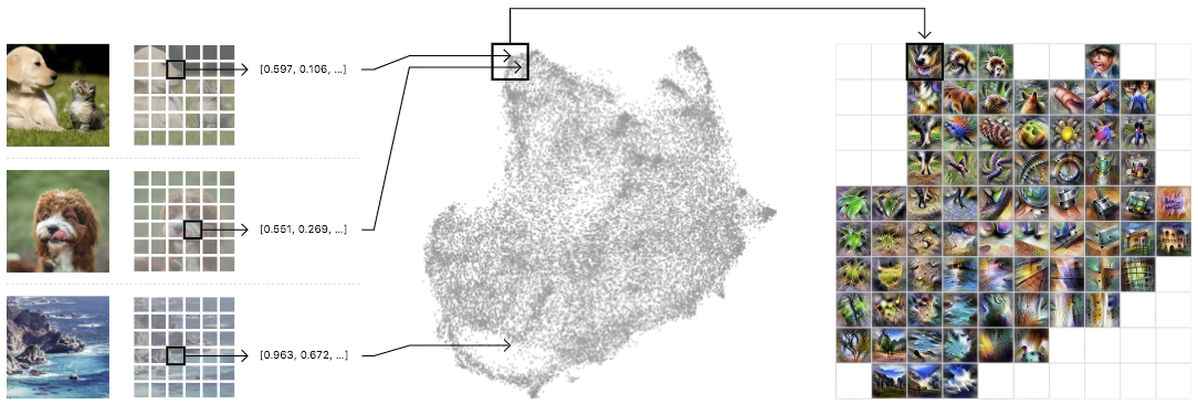 |
| Left: A randomized set of one million images is fed through the network, collecting one random spatial activation per image. Center: The activations are fed through UMAP to reduce them to two dimensions. They are then plotted, with similar activations placed near each other. Right: We then draw a grid, average the activations that fall within a cell, and run feature inversion on the averaged activation. |
Below we can see an activation atlas for just one layer in a neural network (remember that these classification models can have half a dozen or more layers). It reveals a universe of the visual concepts the network has learned to classify images at this layer. This atlas can be a bit overwhelming at first glance — there’s a lot going on! This diversity is a reflection of the variety of visual abstractions and concepts the model has developed.
 |
| An overview of an activation atlas for one of the many layers (mixed4c) within Inception v1. It is about halfway through the network. |
 |
| In this detail, we can see detectors for different types of leaves and plants. |
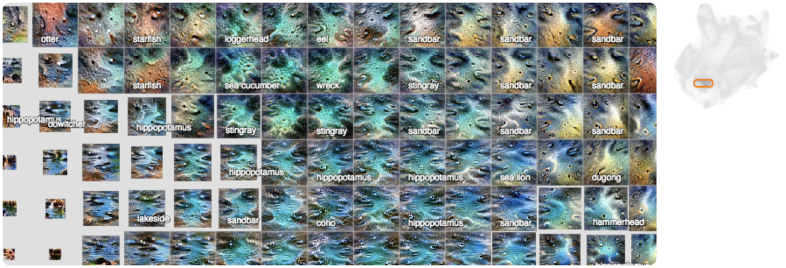 |
| Here we can see different detectors for water, lakes and sandbars. |
 |
| Here we see different types of buildings and bridges. |
As we mentioned before, there are many more layers in this network. Let’s look at the layers that came before this one to see how these concepts become more refined as we go deeper into the network (Each layer builds its activations on top of the preceding layer’s activations).
 |
| In an early layer, mixed4a, there is a vague “mammalian” area. |
 |
| By the next layer in the network, mixed4b, animals and people have been disentangled, with some fruit and food emerging in the middle. |
 |
| By layer mixed4c these concepts are further refined and differentiated into small “peninsulas”. |
Here we’ve seen the global structure evolve from layer to layer, but each of the individual concepts also become more specific and complex from layer to layer. If we focus on the areas of three layers that contribute to a specific classification, say “cabbage”, we can see this clearly.
 |
| Left: This early layer is very nonspecific in comparison to the others. Center: By the middle layer, the images definitely resemble leaves, but they could be any type of plant. Right: By the last layer the images are very specific to cabbage, leaves curved into rounded balls. |
There is another phenomenon worth noting: not only are concepts being refined as you move from layer to layer, but new concepts seem to be appearing out of combinations of old ones.
 |
| You can see how sand and water are distinct concepts in a middle layer, mixed4c (left and center), both with strong attributions to the classification of “sandbar”. Contrast this with a later layer (right), mixed5b, where the two ideas seem to be fused into one activation. |
Instead of zooming in on certain areas of the whole atlas for a specific layer, we can also create an atlas at a specific layer for just one of the 1,000 classes in ImageNet. This will show the concepts and detectors that the network most often uses to classify a specific class, say “red fox” for instance.
 |
| Here we can more clearly see what the network is focusing on to classify a “red fox”. There are pointy ears, white snouts surrounded by red fur, and wooded or snowy backgrounds. |
 |
| Here we can see the many different scales and angles of detectors for “tile roof”. |
 |
| For “ibex”, we see detectors for horns and brown fur, but also environments where we might find such animals, like rocky hillsides. |
 |
| Like the detectors for tile roof, “artichoke” also has many different sizes of detectors for the texture of an artichoke, but we also get some purple flower detectors. These are presumably detecting the blossoms of an artichoke plant. |
These atlases not only reveal nuanced visual abstractions within a model, but they can also reveal high-level misunderstandings. For example, by looking at an activation atlas for a “great white shark” we water and triangular fins (as expected) but we also see something that looks like a baseball. This hints at a shortcut taken by this research model where it conflates the red baseball stitching with the open mouth of a great white shark.

We can test this by using a patch of an image of a baseball to switch the model’s classification of a particular image from “grey whale” to “great white shark”.

We hope that activation atlases will be a useful tool in the quiver of techniques that are making machine learning more accessible and interpretable. To help you get started, we’ve released several jupyter notebooks which can be executed immediately in your browser with one click via colab. They build upon the previously released toolkit Lucid, which includes code for many other interpretability visualization techniques included as well. We’re excited to see what you discover!
Easily perform bulk label quality assurance using Amazon SageMaker Ground Truth
In this blog post we’re going to walk you through an example situation where you’ve just built a machine learning system that labels your data at volume and you want to perform manual quality assurance (QA) on some of the labels. How can you do so without overwhelming your limited resources? We’ll show you how, by using an Amazon SageMaker Ground Truth custom labeling job.
Rather than asking your workers to validate items one at a time, you’ll accomplish custom labeling by presenting a small batch of already-labeled items that have been assigned the same label. You’ll ask the worker to mark any that aren’t correct. In this way, a workforce is able to quickly assess a much larger quantity of data than they could label from scratch in the same time.
Use case tasks that might require quality assurance include:
- Requiring subject matter expert review and approval of labels before using them for sensitive use cases.
- Reviewing the labels to test the quality of the label-producing model.
- Identifying and counting mislabeled items, correcting them, and feeding them back into the training set.
- Analyzing label correctness versus confidence levels assigned by the model.
- Understanding whether a single threshold can be applied to all label classes, or whether using different thresholds for different classes is more appropriate.
- Exploring the use of a simpler model to label some initial data, then improving the model by using QA to validate the results and retrain.
In this blog post, you’ll walk through an example that addresses these use cases.
Background and solution overview
Amazon SageMaker Ground Truth offers easy access to public and private human labelers and provides them with built-in workflows and interfaces for common labeling tasks. In this blog post, you leverage and extend a Ground Truth Custom Labeling Workflow to support another time-consuming part of an overall system or business process: quality assurance of labels that have been applied, either via machine learning or by human labelers.
The input in this sample case is a list of labeled images to be validated by your private workforce. A worker sees a batch of images with a single label presented on a single screen, so they can validate a set of labels at a time. They can quickly scan the entire set and mark any that are not correctly labeled, picking out the ones that don’t “fit.” The validated results are stored in an Amazon DynamoDB table. Note that the volume of items in a batch should be chosen appropriately for the task, depending on their complexity and ability to be displayed for easy comparison and review. For our example, the batch size was chosen as 25 (configurable in the template) to balance cognitive load with the volume of images to be reviewed.
Anatomy of an Amazon SageMaker Ground Truth custom labeling job
An Amazon SageMaker Ground Truth custom labeling workflow consists of the following components:
- A workforce, to perform the labeling tasks. You can choose from a public workforce (for example, by using Amazon Mechanical Turk), or a private workforce.
- A JSON manifest file. The manifest tells Ground Truth where to find the job inputs. Each line item is a single object and corresponds to a single task. In our example, each object is a custom labeling input that points to a batch of images with the same label that will be presented to the worker at the same time for QA.
- A pre-labeling task AWS Lambda function. Before a labeling task is sent to the worker, your AWS Lambda pre-labeling function will be sent a JSON-formatted request to provide details. This JSON request must contain all the details the function will need in order to pass to the custom labeling job template.
- A custom labeling task template. The template defines what will be shown to the worker during the labeling task. The inputs to the task are made available to the template by the pre-labeling task Lambda function.
- A post-labeling task Lambda function. When the worker has completed the task, Ground Truth will send the results to your post-labeling task Lambda function. This Lambda function is generally used for annotation consolidation. The actual annotation data will be stored in a file designated by the s3Uri string in the payload object.
After these components are set up, you can create a Ground Truth labeling job that specifies these components. Ground Truth takes care of sending the individual labeling tasks to the workers and consolidating the outputs.
Solution overview
For the use case described in this blog post, the input to this process is images that have already been labeled by a machine learning model such as Amazon Rekognition, with a label and the confidence score the model had in assigning the label.
In this example, you’ll use a subset of the CalTech 101[i] dataset from AWS Open Datasets for image classification, which we’ve prelabeled for you. A corpus input file has been provided that specifies the subset of images to use and their labels. For example, our model had taken the following images and labeled them as “Crawdad”:
Now, you’re interested in assessing the quality of the labels that have been applied.
The following diagram shows the overall process flow.
- In steps 1, 2 and 3, users identify images and upload them.
- In step 4, a model analyzes the images and labels them (step 5).
- In step 6, labels and images are aggregated and Ground Truth labeling jobs created.
- A workforce of labelers reviews the labels in step 7.
- In step 8a, the results are sent back to the model for retraining.
- In step 8b, the results are analyzed by data scientists to better understand model behavior, and by the business to understand how the model’s inferences in the production system should be best used.
In the remainder of this blog post, we’ll walk you through an implementation that focuses on steps 6 and 7. You’ll also look at the results, step 8b.
Using the Amazon SageMaker Ground Truth custom labeling job for QA
In this section you’ll set up and execute the implementation components, shown in the figure that follows. The solution implementation uses two major components:
- An Amazon SageMaker Ground Truth custom labeling workflow.
- An Amazon DynamoDB table, used to store the results of the labeling task.
For ease of use, a Lambda function prepopulates an Amazon S3 bucket and an Amazon DynamoDB table for you.
You’ll execute the following steps:
- First, you’ll create a private workforce (1), using the AWS Management Console.
- Then, you’ll execute a provided AWS CloudFormation stack to set up resources: the Amazon S3 bucket containing job inputs, a DynamoDB table to hold the results, and the Pre-Labeling and Post-Labeling Lambda functions for use by Ground Truth. The stack will also run a Lambda function (Launch) to pre-populate the job manifests (2).
- You’ll create a Ground Truth labeling job that reads the manifest (3).
- Ground Truth then prepares the labeling tasks by sending them to the pre-labeling Lambda function and sends them to the workers (4).
- You’ll perform the label quality assurance step (5), acting as the private workforce (5).
- Ground Truth will send the worker-labeled data to the post-labeling Lambda function (6), which writes the worker-assigned labels to the DynamoDB label table (7)
- Lastly, you’ll review the results of the labeling task.
Here are the details. You can also see the source code here.
Create a private workforce
To set up your private workforce, use the AWS Management Console. Choose the Region us-east-1 (the workforce must be created in the Region where the code resides). Follow the instructions under “Creating a workforce using the console” under Managing a Private Workforce, using any of the three options presented. This step also creates a labeling portal sign-in URL. You’ll need this URL later.
Create a new team, called bulkQA. Add one worker: yourself. Add your email, and complete the registration step.
Set up resources
To see this solution in operation in us-west-2, choose the Launch Stack button that follows.
Cost: Note that the total solution costs around $1.00 to run. Remember to delete the CloudFormation stack when you’ve finished with the solution.
![]()
Choose Next. Check that the parameters shown in the following screenshot will work for your environment.
Finally, review all the settings on the next page. Select the box marked I acknowledge that AWS CloudFormation might create IAM resources (this is required since the script creates IAM resources), then choose Create.
Wait until the stack launch is complete, and look at the stack Outputs tab.
You’ll see the stack has created the following resources:
- An Amazon Simple Storage Service (S3)bucket (key = BulkQABucket). This bucket now contains:
- A JSON file, manifest.json, that has been generated for you. This file contains a list of the custom labeling inputs. Each of these custom labeling inputs will become a separate Ground Truth labeling task within the overall labeling job.
- A series of folders containing images. These folders contain a batch of images that have been copied from the CalTech 101 dataset, for use during this labeling project.
- A folder called custom_labeling_inputs. This folder contains a set of JSON files that have been generated for you. Each file contains a batch of images that have been assigned the same label, along with the confidence the model had in that label, and the S3 location of the source image. For example:
Each custom labeling input will become a single task in Ground Truth (subject to the chosen batch size) that shows all images listed in the array along with the label to the worker for confirmation.
- An AWS Identity and Access Management (IAM) role (key = SageMakerRoleARN), to be used by the Ground Truth custom labeling job.
- A DynamoDB table (key = DynamoDBLabelTableName). The table has been preloaded with the list of images on S3, the label, and the label confidence assigned by the source labeling model. These are the labels that you want to confirm.

In addition, the stack has created three Lambda functions. They are:
- rLambdaLaunchFunction. This Lambda function is run one time during the CloudFormation stack launch, to set up the environment for this use case. It takes as input a CSV file that contains three columns: image filename, label, and confidence. For each line item, it copies the image file to S3. It also creates an entry for that line item in DynamoDB, and creates the manifest files.
- rLambdaGTPreLabelingFunction. This Lambda function is run at the beginning of each custom labeling task. As input, it receives from Ground Truth the S3 URI of one of the custom labeling inputs. It reads the manifest from S3 and passes the contents to Ground Truth, wrapped in a JSON object:
- rLambdaGTPostLabelingFunction. This Lambda function is run after a labeling task has been completed and consolidates the worker’s annotations. In this case, it simply reads the worker’s annotations and updates them in the DynamoDB table.

Now that these components have been created, you’re ready to create the custom labeling job.
Create the custom labeling job
In the AWS Management Console, go to the Amazon SageMaker console. In the left navigation bar, choose Ground Truth, then choose Labeling Jobs. Choose Create Labeling Job.
- Name the job “BulkQATestJob”
- The input dataset is at s3://<BULKQA-BUCKET>/manifest.json
- Set your output dataset location to s3://<BULKQA-BUCKET>/output/
- For the IAM Role, choose to enter a custom Role ARN. Copy the ARN for the SageMakerExecutionRole generated by CFN here.

- Scroll down. Under Task Type, choose Custom.

- Choose Next.
On the Select workers and configure tool page:
- Under Workers, choose worker type of Private.
- Under Private teams, choose the team you set up previously.

Scroll down. Under Custom labeling task setup:
- Choose a template type of Custom.
- Copy and paste the full text of the bulkqa html template shown below.
The code here is just a few lines in length. The crowd-form tag wraps the custom task code. It reads the label for this set from task.input.sourceRef[0].label and uses that text to create the page instruction. A for-loop then creates a crowd-card for each image listed in the input custom_labeling_input this task received as input, and places a pre-checked check box under each image.
- Under Pre-labeling task Lambda function, choose the LambdaGTPreLabelingFunction from the drop-down list.
- Under Post-labeling task Lambda function, choose the LambdaGTPostLabelingFunction from the drop-down list.

- Choose Submit.
Ground Truth now shows the job status as In progress, with a no (blank) labeled objects/total.
Wait for a few minutes while Ground Truth validates that your job works. After a few minutes, the Labeled objects/total column in the UI should change to contain a count, such as: 0 / 9. The total is the number of Ground Truth custom labeling inputs that your workers will QA. Here, each class label may be one or more images, depending on the size you chose for the QA batch size.
Now your workforce should start receiving labeling tasks within a few minutes.
Confirming the image labels
In the AWS Management Console left navigation bar, choose Ground Truth Labeling workforces. Choose the Private tab. Under the Private workforce summary, choose the Labeling portal sign-in URL.
Sign in with your workforce user name and password. You should see a job listed. If you don’t, wait a few more minutes and refresh the page. Repeat until the data labeling job becomes available.
Choose Start Working.
For each assigned task, the worker web page presents a set of images, each of which has been assigned the same label. In the first example image below, it is cat, in the second, crab. Each image has a Confirm check box below the image. These check boxes are checked by default.
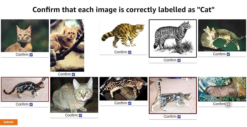
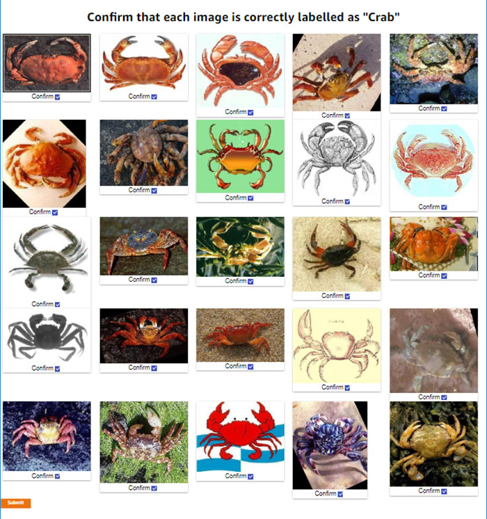
Review the images. For any image that does not match the label, uncheck the check box. When you’ve reviewed all the images on the page, choose Submit.
Behind the scenes, the post-labeling Lambda function runs. This Lambda function updates the DynamoDB table with the results. It adds up to two fields to each row: WorkerConfirmCount and WorkerDisconfirmCount. These columns are updated with the number of reviewers who have confirmed or disconfirmed each individual image.
Continue until all tasks have been completed. Ground Truth will batch the tasks, and then wait before assigning the next batch. If there are more than 10 tasks you will probably need to wait before the next batch becomes available to you.
Assessing the results
After all the tasks have been completed, the final results are ready for review in the DynamoDB table. In the AWS Management Console, navigate to the Amazon DynamoDB console. Under Tables, choose the BulkQALabelTable created earlier. Choose the Items tab, and review the table along with the worker confirmations.
In the screenshot of the DynamoDB console that follows, you can see that one worker has disconfirmed two of the images and has confirmed a third.
Having a single worker confirm the results might be reasonable if the worker is highly trained or otherwise considered an authoritative source of truth. Alternatively, for a sensitive use case or where your workers are less authoritative, you might want to have a larger number of workers – say, three – validate the results, and only use the ones that all have confirmed as correct.
Cleanup
After you have finished reviewing the results of this test, remember to delete the CloudFormation template. Doing so will remove the DynamoDB table and created S3 bucket, and prevent continuing charges.
Acting on the results
In this section we show you results from a specific assessment of the two larger samples. These were assessments from specific “experts,” so your results might vary. The two sample files are provided, and can be run by replacing bulkqa/smallsample.csv with their names in the CloudFormation template:
- bulkqa/sample.csv contains 10 classes and 510 images
- bulkqa/shellfish.csv contains 5 classes of shellfish, and 245 images.
These samples have more classes and more images, so they will take longer to assess. Ground Truth will send objects to your workers in batches. That is, it will assign some number of tasks – often 10 – to a worker, and then take a break before assigning the next set.
This method identifies false positives in any group. False negatives (images that should have been assigned to this class but were not) are not identified by this approach. You could add identifying the correct class (for example, out of a list of possible classes) to this method, at the cost of slowing down the QA process and potentially slowing down how quickly correctly classified items become available for use by the business. Alternatively, you could chain a separate process step that assigns the correct class for each misclassified item, for example by using the Ground Truth classification workflow. Whether this is appropriate depends on the reason for the QA process.
The now-labeled-and-confirmed data can be fed back into the model and used for retraining. In the cases where this gives you a more accurate model, this is the preferred approach. However, it is also possible that the existing model is already optimal, or that adding additional training examples does not improve overall model performance but merely moves the errors to a different class.
Another scenario is when you are interested in differences between the classes, beyond the accuracy of individual label or the average performance across the model. The following table shows a simple bucketing of the images by class and confidence score obtained by running the provided sample.csv input. Any images where the workers were split is treated as Incorrect in the bucketing. Note that only images with a confidence score of 80 or higher were passed into the QA process; in essence, the input process uses a base threshold of 80.
| Total | 80-85 Confidence | 85-90 Confidence | 90-95 Confidence | 95-100 Confidence | |||||||||||||
| Label | Total | Confirmed | Disconfirm | Split | %Correct | Total | Incorrect | %Correct | Total | Incorrect | %Correct | Total | Incorrect | %Correct | Total | Incorrect | %Correct |
| Beaver | 28 | 27 | 1 | 1 | 96.43% | 2 | 1 | 50.00% | 3 | 0 | 100.00% | 13 | 0 | 100.00% | 10 | 0 | 100.00% |
| Cat | 10 | 9 | 1 | 3 | 90.00% | 1 | 1 | 0.00% | 0 | 0 | 0.00% | 5 | 0 | 100.00% | 4 | 0 | 100.00% |
| Crawdad | 68 | 35 | 33 | 4 | 51.47% | 1 | 1 | 0.00% | 10 | 8 | 20.00% | 10 | 6 | 40.00% | 47 | 19 | 59.57% |
| Dinosaur | 65 | 62 | 3 | 5 | 95.38% | 4 | 0 | 100.00% | 10 | 1 | 90.00% | 12 | 1 | 91.67% | 39 | 1 | 97.44% |
| Dog | 68 | 67 | 1 | 6 | 98.53% | 1 | 0 | 100.00% | 5 | 1 | 80.00% | 34 | 0 | 100.00% | 28 | 1 | 96.43% |
| Saxophone | 40 | 38 | 1 | 7 | 95.00% | 1 | 0 | 100.00% | 2 | 1 | 50.00% | 22 | 1 | 95.45% | 15 | 0 | 100.00% |
| Sea Turtle | 86 | 84 | 1 | 8 | 97.67% | 5 | 1 | 80.00% | 8 | 1 | 87.50% | 13 | 0 | 100.00% | 60 | 0 | 100.00% |
| Soccer Ball | 87 | 69 | 18 | 11 | 79.31% | 8 | 5 | 37.50% | 7 | 5 | 28.57% | 9 | 6 | 33.33% | 63 | 2 | 96.83% |
| Stop sign | 58 | 58 | 0 | 12 | 100.00% | 6 | 0 | 100.00% | 9 | 0 | 100.00% | 12 | 0 | 100.00% | 31 | 0 | 100.00% |
| TOTALS | 510 | 449 | 59 | 57 | 88.04% | 29 | 9 | 68.97% | 54 | 17 | 68.52% | 130 | 14 | 89.23% | 297 | 23 | 92.26% |
| Class Average | 89.31% | 63.06% | 61.79% | 84.49% | 94.47% | ||||||||||||
Some interesting patterns are immediately visible, and raise questions for further analysis and assessment.
The classes Cat and Beaver are underrepresented in the input. Is this because they are under-represented in the original model input, or are they receiving confidence scores lower than 80 and thus not coming to the QA process? Or, are these rare cases in the source of the model input? (In the case of Cat, this seems intuitively unlikely.)
There are large differences between the percentage correct at different confidence levels across the classes. For example, all stop signs are correct, whereas even at confidence scores between 95 and 100, around half of crawdads are incorrect. An initial hypothesis is that some classes may be more easily confused. For example, saxophones are more distinctive than crawdads versus crabs, which may be harder for a human or a non-expert to correctly identify. To test this hypothesis a second assessment, using shellfish.csv, is shown in the following table.
| Total | 80-85 Confidence | 85-90 Confidence | 90-95 Confidence | 95-100 Confidence | |||||||||||||
| Label | Total | Confirmed | Disconfirm | Split | %Correct | Total | Incorrect | %Correct | Total | Incorrect | %Correct | Total | Incorrect | %Correct | Total | Incorrect | %Correct |
| Crab | 45 | 45 | 0 | 0 | 100.00% | 4 | 0 | 100.00% | 7 | 0 | 100.00% | 11 | 0 | 100.00% | 23 | 0 | 100.00% |
| Crawdad | 68 | 16 | 32 | 20 | 23.53% | 1 | 0 | 100.00% | 10 | 8 | 20.00% | 10 | 8 | 20.00% | 47 | 36 | 23.40% |
| Lobster | 53 | 40 | 11 | 2 | 75.47% | 4 | 4 | 0.00% | 10 | 4 | 60.00% | 11 | 3 | 72.73% | 28 | 2 | 92.86% |
| Scorpion | 77 | 72 | 3 | 2 | 93.51% | 8 | 3 | 62.50% | 6 | 2 | 66.67% | 27 | 0 | 100.00% | 36 | 0 | 100.00% |
| Shrimp | 2 | 0 | 1 | 1 | 0.00% | 0 | 0 | 0.00% | 1 | 1 | 0.00% | 0 | 0 | 0.00% | 1 | 1 | 0.00% |
| TOTALS | 245 | 173 | 47 | 25 | 70.61% | 17 | 7 | 58.82% | 34 | 15 | 55.88% | 59 | 11 | 81.36% | 135 | 39 | 71.11% |
| Class Average | 58.50% | 52.50% | 49.33% | 58.55% | 63.25% | ||||||||||||
Interestingly, this assessment shows that all crabs are correctly identified, almost all scorpions were correctly identified, whereas no shrimp (of the 2) were correctly identified. The model appears to be having particular difficulty with crawdads. Perhaps a second, more specific model needs to be trained to specifically focus on crawdads and the classes it frequently misidentifies. All images classified as crawdads by the initial model could then be pipelined to the second model for reclassification.
Perhaps the input images for these classes have systemic differences, such as underwater shots or poor lighting for crawdads. Or perhaps the model has classification biases. Since the model was originally built via transfer learning, perhaps the model that was transferred was trained on a significantly different corpus, and some additional training is warranted.
In a setting where class differences or bias matter (for example, see Corbett and Davies, The Measure and Mismeasure of Fairness), using a global threshold (such as the ‘80’ used here) might not be appropriate.
For example, say the business wishes to ensure that they have classification parity for each class. That is, they wish to have approximately the same error rate (the same ratio of false positives to true positives) for items above each class’ threshold. Clearly, given the previous data, using the same threshold for crawdads, lobsters, and stop signs will not achieve this goal. Say that they estimate the costs associated with processing a false positive are 10 times that of processing a true positive. To achieve this, you need to identify an appropriate threshold for each class. Intuitively, since all stop signs were correctly identified, the global threshold of 80 is appropriate for the stop sign class. For crawdads, closer inspection reveals that even above a confidence of 99.5, there are too many errors. The pipeline method described above should be applied before sending any crawdad-labeled images to the business.
One approach to identifying an appropriate threshold for these classes is the following. Begin with the rightmost bucket. If the ratio of incorrectly classified images is lower than the business will accept, move to the next-left bucket and repeat. If not – stop and use the high side of the current bucket as the threshold. For the 1:10 ratio and the class of cat (overlooking the small size of this class for now), this gives a class threshold of 85. See On Calibration of Modern Neural Networks for alternate approaches and deeper analysis.
Conclusion
In this blog post you’ve seen how to use Amazon SageMaker Ground Truth custom labeling workflows to easily perform bulk quality assurance of your labels. Using this approach, you can quickly validate the prior labels assigned, and feed the results back to improve the quality of your model. Or, you can use this approach to validate labels for sensitive business use cases.
You’ve also seen how to use this approach to study whether a single threshold is appropriately used across all of the label classes your model assigns, or whether some classes should have a higher threshold assigned to achieve classification parity.
By using these approaches, you can improve the quality of your models, and use your models with confidence in a wider range of business use cases. Enjoy!
[i] L. Fei-Fei, R. Fergus and P. Perona. Learning generative visual models from few training examples: an incremental Bayesian approach tested on 101 object categories. IEEE. CVPR 2004, Workshop on Generative-Model Based Vision. 2004
About the Authors
 Veronika Megler is a Principal Consultant, Big Data, Analytics & Data Science, for AWS Professional Services. She holds a PhD in Computer Science, with a focus on spatio-temporal data search. She specializes in technology adoption, helping customers use new technologies to solve new problems and to solve old problems more efficiently and effectively.
 Chris Ghyzel is a Data Engineer for AWS Professional Services. Currently, he is working with customers to integrate machine learning solutions on AWS into their production pipelines.
Introducing GPipe, an Open Source Library for Efficiently Training Large-scale Neural Network Models
Deep neural networks (DNNs) have advanced many machine learning tasks, including speech recognition, visual recognition, and language processing. Recent advances by BigGan, Bert, and GPT2.0 have shown that ever-larger DNN models lead to better task performance and past progress in visual recognition tasks has also shown a strong correlation between the model size and classification accuracy. For example, the winner of the 2014 ImageNet visual recognition challenge was GoogleNet, which achieved 74.8% top-1 accuracy with 4 million parameters, while just three years later, the winner of the 2017 ImageNet challenge went to Squeeze-and-Excitation Networks, which achieved 82.7% top-1 accuracy with 145.8 million (36x more) parameters. However, in the same period, GPU memory has only increased by a factor of ~3, and the current state-of-the-art image models have already reached the available memory found on Cloud TPUv2s. Hence, there is a strong and pressing need for an efficient, scalable infrastructure that enables large-scale deep learning and overcomes the memory limitation on current accelerators.
 |
| Strong correlation between ImageNet accuracy and model size for recently developed representative image classification models |
In “GPipe: Efficient Training of Giant Neural Networks using Pipeline Parallelism“, we demonstrate the use of pipeline parallelism to scale up DNN training to overcome this limitation. GPipe is a distributed machine learning library that uses synchronous stochastic gradient descent and pipeline parallelism for training, applicable to any DNN that consists of multiple sequential layers. Importantly, GPipe allows researchers to easily deploy more accelerators to train larger models and to scale the performance without tuning hyperparameters. To demonstrate the effectiveness of GPipe, we trained an AmoebaNet-B with 557 million model parameters and input image size of 480 x 480 on Google Cloud TPUv2s. This model performed well on multiple popular datasets, including pushing the single-crop ImageNet accuracy to 84.3%, the CIFAR-10 accuracy to 99%, and the CIFAR-100 accuracy to 91.3%. The core GPipe library has been open sourced under the Lingvo framework.
From Mini- to Micro-Batches
There are two standard ways to speed up moderate-size DNN models. The data parallelism approach employs more machines and splits the input data across them. Another way is to move the model to accelerators, such as GPUs or TPUs, which have special hardware to accelerate model training. However, accelerators have limited memory and limited communication bandwidth with the host machine. Thus, model parallelism is needed for training a bigger DNN model on accelerators by dividing the model into partitions and assigning different partitions to different accelerators. But due to the sequential nature of DNNs, this naive strategy may result in only one accelerator being active during computation, significantly underutilizing accelerator compute capacity. On the other hand, a standard data parallelism approach allows concurrent training of the same model with different input data on multiple accelerators, but cannot increase the maximum model size an accelerator can support.
To enable efficient training across multiple accelerators, GPipe partitions a model across different accelerators and automatically splits a mini-batch of training examples into smaller micro-batches. By pipelining the execution across micro-batches, accelerators can operate in parallel. In addition, gradients are consistently accumulated across micro-batches, so that the number of partitions does not affect the model quality.
 |
Top: The naive model parallelism strategy leads to severe underutilization due to the sequential nature of the network. Only one accelerator is active at a time. Bottom: GPipe divides the input mini-batch into smaller micro-batches, enabling different accelerators to work on separate micro-batches at the same time. |
Maximizing Memory and Efficiency
GPipe maximizes memory allocation for model parameters. We ran the experiments on Cloud TPUv2s, each of which has 8 accelerator cores and 64 GB memory (8 GB per accelerator). Without GPipe, a single accelerator can train up to 82 million model parameters due to memory limits. Thanks to recomputation in backpropagation and batch splitting, GPipe reduced intermediate activation memory from 6.26 GB to 3.46GB, enabling 318 million parameters on a single accelerator. We also saw that with pipeline parallelism the maximum model size was proportional to the number of partitions, as expected. With GPipe, AmoebaNet was able to incorporate 1.8 billion parameters on the 8 accelerators of a Cloud TPUv2, 25x times more than is possible without GPipe.
To test efficiency, we measured the effects of GPipe on the model throughput of AmoebaNet-D. Since training required at least two accelerators to fit the model size, we measured the speedup with respect to the naive case with two partitions but no pipeline parallelization. We observed an almost linear speedup in training. Compared to the naive approach with two partitions, distributing the model across four times the accelerators achieved a speedup of 3.5x. While all experiments in our paper used Cloud TPUv2, we see even better performance with the currently available Cloud TPUv3s, each of which has 16 accelerator cores and 256 GB (16 GB per accelerator). GPipe enabled 8 billion parameter Transformer language models on 1024-token sentences with a speedup of 11x when distributing the model across all sixteen accelerators.
 |
Speedup of AmoebaNet-D using GPipe. This model could not fit into one accelerator. The baseline naive-2 is the performance of the native partition approach when the model is split into two partitions. Pipeline-k refers to the performance of GPipe that splits the model into k partitions with k accelerators. |
GPipe can also scale training by employing even more accelerators without changes in the hyperparameters. Therefore, it can be combined with data parallelism to scale neural network training using even more accelerators in a complementary way.
Testing Accuracy
We used GPipe to verify the hypothesis that scaling up existing neural networks can achieve even better model quality. We trained an AmoebaNet-B with 557 million model parameters and input image size of 480 x 480 on the ImageNet ILSVRC-2012 dataset. The network was divided into 4 partitions and applied parallel training processes to both model and data. This giant model reached the state-of-the-art 84.3% top-1 / 97% top-5 single-crop validation accuracy without any external data. Large neural networks are not only applicable to datasets like ImageNet, but also relevant for other datasets through transfer learning. It has been shown that better ImageNet models transfer better. We ran transfer learning experiments on the CIFAR10 and CIFAR100 datasets. Our giant models increased the best published CIFAR-10 accuracy to 99% and CIFAR-100 accuracy to 91.3%.
Conclusion
The ongoing development and success of many practical machine learning applications, such as autonomous driving and medical imaging, depend on achieving the highest accuracy possible. As this often requires building larger and even more complex models, we are happy to provide GPipe to the broader research community, and hope it is a useful infrastructure for efficient training of large-scale DNNs.
Acknowledgments
Special thanks to the co-authors of the paper: Youlong Cheng, Dehao Che, HyoukJoong Lee, Jiquan Ngiam, Quoc V. Le, and Zhifeng Chen. We wish to thank Esteban Real, Alok Aggarwal, Xiaodan Song, Naveen Kumar, Mark Heffernan, Rajat Monga, Megan Kacholia, Samy Bengio, and Jeff Dean for their support and valuable input; Noam Shazeer, Patrick Nguyen, Xiaoqiang Zheng, Yonghui Wu, Barret Zoph, Ekin Cubuk, Jonathan Shen, Tianqi Chen, and Vijay Vasudevan for helpful discussions and inspirations; and the larger Google Brain team.
Improving Patient Care with Machine Learning At Beth Israel Deaconess Medical Center
Beth Israel Deaconess Medical Center has launched a multi-year, innovative research program on how machine learning can improve patient care, supported by an academic research sponsorship grant from AWS. The Harvard Medical School-affiliated teaching hospital will use a broad array of AWS machine learning services to uncover new ways that machine learning technology can enhance clinical care, streamline operations, and eliminate waste, with the goal of improving patient care and quality of life.
Improving patient care with machine learning
Inefficiencies in hospital management and operations are not only extremely costly to providers, insurers, patients, and taxpayers, but they can result in precious resources being diverted away from patient care. These inefficiencies drive healthcare costs up and can contribute to life-threatening medical errors.
The work now underway at BIDMC strives to identify new methods that can be shared across the healthcare industry, with the goals of advancing better patient outcomes, decreasing hospitalizations and readmissions, and lowering health care costs for all Americans. BIDMC’s machine learning research seeks to create data-based solutions and processes to address these challenges, be scalable across the healthcare industry, and further enhance patient care.
An initial BIDMC research project used machine learning to optimize the schedules of its 41 operating rooms and align those schedules to improve patient flow in the inpatient setting. Another project has leveraged machine learning to improve operational flow within operating rooms. Now, incoming pre-surgical document packages will be scanned as images and processed with TensorFlow on Amazon SageMaker, hosted in BIDMC’s secure AWS cloud. This machine learning driven process automatically recognizes and inserts consent forms into corresponding electronic health records (EHR), saving hospital staff hours of manual work. BIDMC built a model that scans EHRs to look for key elements like a completed consent form. If a consent form isn’t found, a signal appears on the EHR and nurses follow up with those patients.
Similarly, BIDMC has more than 490 inpatient medical/surgical beds that are highly occupied, and its team strives to successfully perform surgical procedures in order that patients can be treated and recover in a timely manner. However, procedures were sometimes delayed or rescheduled because a completed History and Physical (H&P) form, which is required before surgery can start, could be difficult to locate in the documentation that is sometimes faxed to the hospital. To solve this, BIDMC now uses Amazon Comprehend Medical to extract key medical terms and insights that are used in a machine learning model to identify H&Ps. As a result, valuable time can be saved and delays and rescheduling can be prevented.
“Advancements in technology and deep learning have the power to advance care and make a meaningful difference in the lives of thousands of patients and providers,” said Manu Tandon, Chief Information Officer at Beth Israel Deaconess Medical Center.
“Every minute spent on cumbersome clerical tasks and management adds up to millions in lost productivity and directly impacts patient care,” said John Halamka, MD, Executive Director, Health Technology Exploration Center at Beth Israel Deaconess Medical Center and International Healthcare Innovation Professor at Harvard Medical School. “This machine learning research sponsorship will support our commitment to using new and emerging technologies in health care to drive projects that will transform care for patients at BIDMC and around the world.”
Supporting patient adherence and operating room efficiency at BIDMC
Additional projects underway at BIDMC involve predicting which patients are likely to keep their scheduled office appointments and which are not. This project is being built using the Apache MXNet deep learning API and Amazon SageMaker. It will help BIDMC reach out to patients who might miss appointments so that care can be delivered in a timely manner, improving the patient experience and outcomes.
Similarly, BIDMC has developed another machine learning model built on AWS that can detect where simple operating room schedule modifications would improve efficiency, save costs, and balance the load of the hospital during busier times. At the same time, the model can predict the outcome of changes to the schedule and identify what mitigations will minimize negative impacts on patient care.
Making it easier to plan ahead in the Emergency Department
Future projects include assessing the overall level of risk in intensive care units and predicting when the hospital will experience an unexpectedly high volume of incoming patients. For example, BIDMC’s emergency department (ED) typically sees a surge in patient visits during the middle of the week, which can strain hospital resources. BIDMC and academic research partners will analyze datasets, including ED admissions, transfers between healthcare institutions, referrals, pre-scheduled surgeries, patient discharges, and other variables using services such as Amazon QuickSight and Amazon Forecast.
Because of the high volume of data collected, BIDMC will use the AWS Cloud to load and process the necessary data quickly and significantly speed up model training. And using machine learning services like Amazon SageMaker, researchers at BIDMC will build deep learning models that are capable of making highly accurate predictions of where and when space will free up in the hospital for unexpected patients. These projects will help build effective models with the long-term vision of deploying them across the healthcare industry and beyond.
“We are proud to be a part of the innovation happening in healthcare right now and are keen to support organizations like BIDMC who are leading the way in using machine learning technologies to deliver enhanced, personalized care and improved patient experiences,” said Swami Sivasubramanian, Vice President of Machine Learning at AWS. “Supporting BIDMC’s efforts with machine learning services and expertise is a natural extension of the long relationship between our organizations, and we’re excited to help enable their researchers to accelerate the development of models that can advance patient care. BIDMC’s innovations using AWS machine learning services like Amazon SageMaker will ultimately pave the way for other healthcare providers to save lives and reduce costs for patients nationwide.”
AWS is proud to sponsor BIDMC’s research which is a continuation of the company’s mission to put machine learning in the hands of all developers, across the public sector, education, healthcare, and beyond.