Pioneer Corp is a Japanese multinational corporation specializing in digital entertainment products. Pioneer wanted to help their customers check road and traffic conditions through in-car navigation systems. They developed a real-time, image-sharing service to help drivers navigate. The solution analyzes photos, diverts traffic, and sends alerts based on the observed conditions.  Because the pictures are of public roadways, they also had to ensure privacy by blurring out faces and license plate numbers.

Pioneer built their image-sharing service using Amazon SageMaker Neo. Amazon SageMaker is a fully-managed service that provides the ability for developers to build, train, and deploy machine learning models at much less effort and lower cost. Amazon SageMaker Neo is a service that allows developers to train machine learning models once and run them anywhere in the cloud and at the edge. Amazon SageMaker Neo optimizes models to run up to twice as fast, with less than a tenth of the memory footprint, with no loss in accuracy.

You start with an ML model built using MXNet, TensorFlow, PyTorch, or XGBoost and trained using Amazon SageMaker. Then, choose your target hardware platform such as M4/M5/C4/C5 instances or edge devices. With a single click, Amazon SageMaker Neo compiles the trained model into an executable.

The compiler uses a neural network to discover and apply all of the specific performance optimizations to make your model run most efficiently on the target hardware platform. You can deploy the model to start making predictions in the cloud or at the edge.

At launch, Amazon SageMaker Neo was available in four AWS Regions: US East (N. Virginia), US West (Oregon), EU (Ireland), Asia Pacific (Seoul). As of May 2019, SageMaker Neo is now available in Asia Pacific (Tokyo), Japan.

Pioneer developed a machine learning model for real-time image detection and classification using data from cameras in cars. They detect many different kinds of images, such as license plates, people, street traffic, and road signs. The in-car cameras upload data to the cloud and run inference using Amazon SageMaker Neo. The results are sent back to the cars so drivers can be informed on the road.

Here’s how it works.

“We decided to use Amazon SageMaker, a fully managed service for machine learning,” said Ryunosuke Yamauchi, an AI Engineer at Pioneer. “We needed a fully managed service because we didn’t want to spend time managing GPU instances or integrating different applications. In addition, Amazon SageMaker offers hyperparameter optimization, which eliminates the need for time-consuming, manual hyperparameter tuning. Also, we choose Amazon SageMaker because it supports all leading frameworks such as MXNet GluonCV. That’s our preferred framework because it provides state-of-the-art pre-trained object detection models such as Yolo V3.”

To learn more about Amazon SageMaker Neo, see the Amazon SageMaker Neo webpage.

About the Authors

Satadal Bhattacharjee is Principal Product Manager with AWS AI. He leads the Machine Learning Engine PM team working on projects such as SageMaker Neo, AWS Deep Learning AMIs, and AWS Elastic Inference. For fun outside work, Satadal loves to hike, coach robotics teams, and spend time with his family and friends.

Kimberly Madia is a Principal Product Marketing Manager with AWS Machine Learning. Her goal is to make it easy for customers to build, train, and deploy machine learning models using Amazon SageMaker. For fun outside work, Kimberly likes to cook, read, and run on the San Francisco Bay Trail.

Abbott Laboratories has more data than its field team can decipher while on-site with other clients.  Their solution? Working with Smart Bots to build an enterprise-grade, reliable and stable chatbot called Maya, powered by AWS machine learning services like Amazon Lex, AWS Lambda, Amazon Comprehend, and Amazon SageMaker.

For context, Abbott Laboratories is a multinational healthcare company and a forerunner in India in its deployment of AI.  Maya serves Abbott’s 3000+ person field force in India, providing sales operations support and providing access to contextual information at employees’ fingertips.

The chatbot proves especially helpful while employees are in the field meeting doctors. Maya can handle the nitty-gritty of querying and fetching information from enterprise applications so that employees can focus on higher-order tasks.

Maya is integrated with the customer relationship management (CRM) system at Abbott. For each query, the bot gets authenticated on behalf of the user and retrieves the required information.

Amazon Lex enables the language model

Amazon Lex is core to the Maya solution, having been chosen after long discussions regarding the conversation flows and data access protocol from the backend system.

The team identified intents from the conversation flows. Maya today has more than 50 intents—including a “small talk” intent to make the bot more human-like—and close to 250 slots. Most of the intents revolve around data-related actions (for example, filter, compute, and so on). The small talk intent handles phrases like “thank you for your help.”

Lambda determined the response

All 50 intents are linked to a single Lambda function. The following steps are performed on all the requests that call the function.

• Validate the slots based on business rules.
• Call all the subscribed methods related to the newly filled slots.
• Identify the next state.
• Construct the response object.

Lambda acted as the right fit to implement the validation and state flow logic described above.

Session attributes handled context

The team used intent chaining to enhance the conversation flow, which they laud because it makes the bot smarter and streamlines bot management. For those less familiar with this concept, intent chaining facilitates shifting between multiple intents without losing the context. In Maya, context is stored as JSON in the session attributes. The Context object is structured as follows:

sessionAttributes: {
  "context": {
    "previous-context": {
        "primary-context": true,
        "intent-name":"intent-A",
        "slots": {
          "slot-name": "slot-value",
          ...
        },
        "context-variable-1": "value",
        "context-variable-2": "value"
    },
    "current-context": {
        "intent-name":"intent-B",
      "context-variable-3": "value",
      "context-variable-4": "value"
    }
  }
}

* Values in session attributes can only be a string, so the Context JSON object has to be stringified and then assigned.

In the above example, the flow was shifted from intent A to intent B (leaving intent A pending fulfillment). After the current intent (intent B) is fulfilled, the dialogue state goes back to intent A, retaining the previous state.

In real-world terms, this example is applicable in the healthcare space when a user wants to toggle between analysis of a large dataset and individual patient health records. For example, users may want to view the analysis for the causes, symptoms, and likelihood of various diseases.

Results and next steps

With the Maya chatbot deployed in the field, about a third of the queries that medical representatives raise are now answered by Maya rather than a human.

In the coming months, the team looks to further the use of the chatbot and also make it smarter. In particular, they’re looking at using Amazon SageMaker Reinforcement Learning with the Gym interface to facilitate ongoing training while engaging users. The thinking is to prompt a user with what it expects is next set of useful interactions, then reward or penalize the bot based on the relevance of its recommendations.

Amazon SageMaker is also core to a mother-bot architectural approach that is currently being tested. This mother bot is effectively the coordination point that can query the correct child bot to get an answer to the user. This ensemble of bots is expected to perform even better than a single bot handling all the intents. From a technical perspective, the mother bot is a classification algorithm implemented in Amazon SageMaker—a relatively easy task thanks to the streamlined workflow that Amazon SageMaker enables.

About the Author

Marisa Messina is on the AWS AI marketing team, where her job includes identifying the most innovative AWS-using customers and showcasing their inspiring stories. Prior to AWS, she worked on consumer-facing hardware and then university-facing cloud offerings at Microsoft. Outside of work, she enjoys exploring the Pacific Northwest hiking trails, cooking without recipes, and dancing in the rain.

The AWS DeepRacer League is the world’s first global autonomous racing league, open to anyone. Developers of all skill levels can get hands on with machine learning in a fun and exciting way, racing for prizes and glory at 21 events globally and online via the DeepRacer console. The Virtual Circuit launched at the end of April, allowing developers to compete from anywhere in the world via the console – no car or track required – for a chance to top the leaderboard and score points in one of the 6 monthly competitions.

The rubber hits the road for the June race!

On June 3^rd the Kumo Torakku challenge opened, and will be open for racing until June 30^th, at midnight PST. Inspired by the Suzuka circuit in Japan, this track will help developers of all skill levels put their models to the test and advance their knowledge and practice of machine learning. All you need to do is log into the console, where you will be taken through a few quick and easy steps to get your model up and running and ready to race. With the AWS Free Tier you are covered for up to 10 hours of training (in your first 30 days of usage), so you can enter the AWS DeepRacer League at no cost to you.

Once you have learned the basics you will be able to immerse yourself inside the AWS DeepRacer online simulator and watch your model train, until it is ready for submission to the leaderboard. Will it make it round the hairpin, to get views of Mt Fuji? Will you optimize for speed or direction to get the model through the curves? Can you tune your model to take pole position? Get racing today, and don’t forget, if you compete in multiple online races you will score more points, and increase your chances to be eligible for one of the overall Virtual Circuit prizes!

AWS DeepRacer League is open to all and you don’t need the AWS DeepRacer car or to visit an in-person race for a chance to compete, with the virtual circuit you can participate in the race from the comfort of the console. Start your engines, the June race is on!

Watch a successful full lap of the Kumo Torakku, from the AWS DeepRacer 3D online simulator

The Suzuka circuit and the new Kumo Torakku virtual race track

What’s new in the Kumo Torakku?

Aside from enjoying the scenery, you will now have the ability to train your model at a maximum speed of 8 meters per second. But beware, the Kumo Torakku has tight corners and a car travelling at that speed may not be able to take the turns well. It may take time for your model to converge and training time could increase with more throttle, so you will have to experiment with speed in your reward function to help you to succeed. Get started today for your chance to win your expenses paid ticket and join the best of the best at re:Invent 2019.

Cheers to the London Loop winner!

And if that doesn’t inspire you, here’s a quick spotlight and celebration of the May race winner. After a month long race, the London Loop closed on Friday May 31st and the first champion of the virtual tournament was crowned. Karl, who works for the National Australia Bank (NAB) took home the top prize and will now be heading to re:Invent 2019 to join the race for the Championship Cup. At NAB, teams are encouraged to experiment with new concepts and technologies, and the team there have been on their machine learning journey with DeepRacer since it launched at re:Invent 2018. They have created their own DeepRacer community, hosted their own competition, and even saw a team member take third place at the AWS Summit in Sydney.

Karl was joined on the London Loop podium by his teammate Paul, who came third in the May race. Paul recently posted about their experience with the AWS DeepRacer League and you can check it out here. Also be on the lookout for part two where they will share more tips on how to compete to win. Karl, Paul and the rest of the NAB team made a combined 533 attempts to conquer the London Loop challenge. They worked hard on their models, tuning them over time and ultimately clinching the win, and they even said “the virtual league was much more fun than the real race!”

Congratulations to the team and here’s to more AWS DeepRacer success!

About the Author

Alexandra Bush is a Senior Product Marketing Manager for AWS AI. She is passionate about how technology impacts the world around us and enjoys being able to help make it accessible to all. Out of the office she loves to run, travel and stay active in the outdoors with family and friends.

Bewgle is an SAP.iO, Techstars-funded company that uses AWS services to surface insights from user-generated text and audio streams. Bewgle generates insights to help product managers to increase customer satisfaction and engagement with their various products—beauty, electronics, or anything in between.  By listening to the voices of their customers with the help of Bewgle powered by AWS, these product managers are able to drive increased sales for their products.

An average human can read only about 250 words per minute. To synthesize 1000 customer reviews would therefore take upwards of 8 hours. Analyzing the information from all those reviews—plus other text like forum posts and blog posts, as well as unstructured content like survey verbatims and audio streams—quickly becomes untenable.

This is exactly the kind of problem where AI can excel, specifically, the subset of machine learning (ML) called natural language processing (NLP). At the heart of Bewgle’s solution is an AI platform developed completely on AWS that analyzes millions of pieces of content, then extracts key topics and the sentiment behind them. What would otherwise take years can now be done in minutes with Amazon Machine Learning and the AWS tech stack as a whole.

Indeed, the Bewgle solution makes use of a breadth of AWS services. Bewgle’s data processing pipeline relies on AWS Lambda and Amazon DynamoDB, which form the core of the ML tasks involved:

• Storing data for analysis at scale.
• Cleaning up data.
• Firing various processing functions dynamically to generate the analysis.

The team developed an innovative serverless ML workflow to scale the system and orchestrate various workflows in a loosely coupled way. This gave them tremendous agility and flexibility in evaluating and choosing various approaches independently, facilitating speedy innovation.

A typical workflow for Bewgle starts with Amazon SageMaker Ground Truth, which they use to collect and tag data at scale and on demand. The team lauds the high accuracy of the data tagging that Amazon SageMaker Ground Truth delivers. Bewgle co-founder Shantanu Shah explains, “It [Amazon SageMaker Ground Truth] enables efficiency for Bewgle as we no longer have to look for and manage human taggers, and it’s affordable too.”

Once the data tagging is complete, the Bewgle team turns to Amazon SageMaker to reason over it.  They appreciate using the familiar Jupyter Notebook interface to work with the data; they quickly and easily build and test multiple models.  The automatic hyperparameter tuning within Amazon SageMaker greatly speeds and facilitates what would otherwise be a significant effort for the Bewgle team and makes it possible to achieve a high level of accuracy and confidence.

The next step is model deployment, and Amazon SageMaker once again is the solution.  Deploying with Amazon SageMaker is helpful because, in Shah’s words, “Traffic bursts are not an issue as the scalability and redundancy are automatically taken care of.”   He adds, “Overall, [Amazon] SageMaker helps in every step of model building, tuning and serving and saves countless hours of effort for Bewgle.”

This end to end workflow is depicted in the below diagram.

To make the insights available to customers, they built an API using AWS Elastic Beanstalk. The API allows customers to consume the data in any format. A UI layer built on top of the API also allows the customers to view the data as a digest and a dashboard.  With this implementation, listening to user insights at scale becomes easy.  Bewgle users from R&D teams can be smarter in designing new products; product design teams can consider many factors that might otherwise be overlooked; and business development teams can analyze and compare competitor data when determining new features.

Customer support teams are another key user group for Bewgle. Traditional approaches to customer support center mostly or strictly on answering queries related to structured data that they already have (e.g., templatized emails).  Because verbatims (such as comments left by hotel guests) are unstructured data, they cannot contribute to answering customer support queries. Bewgle believes that converting this unstructured text data into structured data is a key to continuously enhancing customer service. Bewgle’s NLP algorithms continuously learn as the data increases, and their output is structured data that is usable by customer service teams. As a tangible example, consider a customer who notes in a feedback form for a product that they could not open the container to access it. The customer service team is able to take that insight and realize that the glue had hardened on a certain batch, making them impossible to open. As such, the company can avoid creating more disgruntled customers (and potentially losing revenue as a result) by removing that batch from the customer-ready pile.

The team is composed of ex-Googlers who founded Bewgle to solve the information overload problem.  The Bewgle crew finds that the AWS AI and ML services enable their workflow to include “less headache” and more impact. The ease of use, documentation, and broad popularity of the AWS tech stack makes it appealing, and the reason for Bewgle’s choice to use AWS as its primary AI/ML platform.

In particular, Shah notes, “Amazon SageMaker allows us to add tremendous flexibility. [Now] we can rapidly iterate on our models as a result and this directly impacts the strength of our company.”

As the awareness of unstructured data analysis, NLP, and AI techniques has grown, Bewgle has seen rapid growth in its business over the last year. Going forward, the team plans to further scale the technology to other verticals and expand to other geographies.

About the Author

Marisa Messina is on the AWS AI marketing team, where her job includes identifying the most innovative AWS-using customers and showcasing their inspiring stories. Prior to AWS, she worked on consumer-facing hardware and then university-facing cloud offerings at Microsoft. Outside of work, she enjoys exploring the Pacific Northwest hiking trails, cooking without recipes, and dancing in the rain.

We are excited to announce the open source release of Gluon Time Series (GluonTS), a Python toolkit developed by Amazon scientists for building, evaluating, and comparing deep learning–based time series models. GluonTS is based on the Gluon interface to Apache MXNet and provides components that make building time series models simple and efficient.

In this post, I describe the key functionality of the toolkit and demonstrate how to apply GluonTS to a time series forecasting problem.

Time series modeling use cases

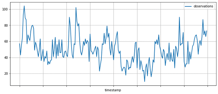
Time series, as the name suggests, are collections of data points that are indexed by time. Time series arise naturally in many different applications, typically by measuring the value of some underlying process at a fixed time interval.

For example, a retailer might calculate and store the number of units sold for each product at the end of each business day. For each product, this leads to a time series of daily sales. An electricity company might measure the amount of electricity consumed by each household in a fixed interval, such as every hour. This leads to a collection of time series of electricity consumption. AWS customers might use Amazon CloudWatch to record various metrics relating to their resources and services, leading to a collection of metrics time series.

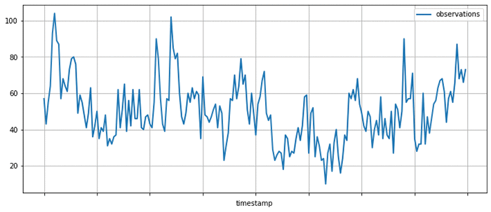
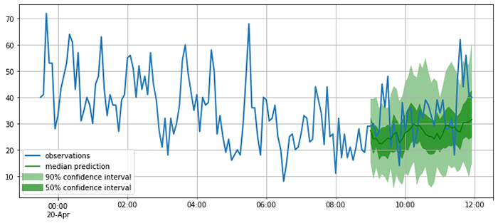
A typical time series may look like the following, where the measured amount is shown on the vertical axis and the horizontal axis is time:

Given a set of time series, you might ask various kinds of questions:

• How will the time series evolve in the future? Forecasting
• Is the behavior of the time series in a given period abnormal? Anomaly detection
• Which group does a given time series belong to? Time series classification
• Some measurements are missing, what were their values? Imputation

GluonTS allows you to address these questions by simplifying the process of building time series models, that is, mathematical descriptions of the process underlying the time series data. Numerous kinds of time series models have been proposed, and GluonTS focuses on a particular subset of these techniques based on deep learning.

GluonTS key functionality and components

GluonTS provides various components that make building deep learning-based, time series models simple and efficient. These models use many of the same building blocks as models that are used in other domains, such as natural language processing or computer vision.

Deep learning models for time series modeling commonly include components such as recurrent neural networks based on Long Short-Term Memory (LSTM) cells, convolutions, and attention mechanisms. This makes using a modern deep-learning framework, such as Apache MXNet, a convenient basis for developing and experimenting with such models.

However, time series modeling also often requires components that are specific to this application domain. GluonTS provides these time series modeling-specific components on top of the Gluon interface to MXNet. In particular, GluonTS contains:

• Higher-level components for building new models, including generic neural network structures like sequence-to-sequence models and components for modeling and transforming probability distributions
• Data loading and iterators for time series data, including a mechanism for transforming the data before it is supplied to the model
• Reference implementations of several state-of-the-art neural forecasting models
• Tooling for evaluating and comparing forecasting models

Most of the building blocks in GluonTS can be used for any of the time series modeling use cases mentioned earlier, while the model implementations and some of the surrounding tooling are currently focused on the forecasting use case.

GluonTS for time series forecasting

To make things more concrete, look at how to use one of time series models that comes bundled in GluonTS, for making forecasts on a real-world time series dataset.

For this example, use the DeepAREstimator, which implements the DeepAR model proposed in the DeepAR: Probabilistic Forecasting with Autoregressive Recurrent Networks paper. Given one or more time series, the model is trained to predict the next prediction_length values given the preceding context_length values. Instead of predicting single best values for each position in the prediction range, the model parametrizes a parametric probability distribution for each output position.

To encapsulate models and trained model artifacts, GluonTS uses an Estimator/Predictor pair of abstractions that should be familiar to users of other machine learning frameworks. An Estimator represents a model that can be trained on a dataset to yield a Predictor, which can later be used to make predictions on unseen data.

Instantiate a DeepAREstimator object by providing a few hyperparameters:

• The time series frequency (for this example, I use 5 minutes, so freq="5min")
• The prediction length (36 time points, which makes it span 3 hours)

You can also provide a Trainer object that can be used to configure the details of the training process. You could configure more aspects of the model by providing more hyperparameters as arguments, but stick with the default values for now, which usually provide a good starting point.

from gluonts.model.deepar import DeepAREstimator
from gluonts.trainer import Trainer

estimator = DeepAREstimator(freq="5min", 
                            prediction_length=36, 
                            trainer=Trainer(epochs=10))

Model training on a real dataset

Having specified the Estimator, you are now ready to train the model on some data. Use a freely available dataset on the volume of tweets mentioning the AMZN ticker symbol. This can be obtained and displayed using Pandas, as follows:

import pandas as pd
import matplotlib.pyplot as plt

url = "https://raw.githubusercontent.com/numenta/NAB/master/data/realTweets/Twitter_volume_AMZN.csv"
df = pd.read_csv(url, header=0, index_col=0)

df[:200].plot(figsize=(12, 5), linewidth=2)
plt.grid()
plt.legend(["observations"])
plt.show()

GluonTS provides a Dataset abstraction for providing uniform access to data across different input formats. Here, use ListDataset to access data stored in memory as a list of dictionaries. In GluonTS, any Dataset is just an Iterable over dictionaries mapping string keys to arbitrary values.

To train your model, truncate the data up to April 5, 2015. Data past this date is used later for testing the model.

from gluonts.dataset.common import ListDataset

training_data = ListDataset(
    [{"start": df.index[0], "target": df.value[:"2015-04-05 00:00:00"]}],
    freq = "5min"
)

With the dataset in hand, you can now use your estimator and call its train method. When the training process is finished, you have a Predictor that can be used for making forecasts.

predictor = estimator.train(training_data=training_data)

Model evaluation

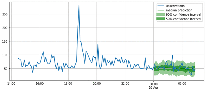
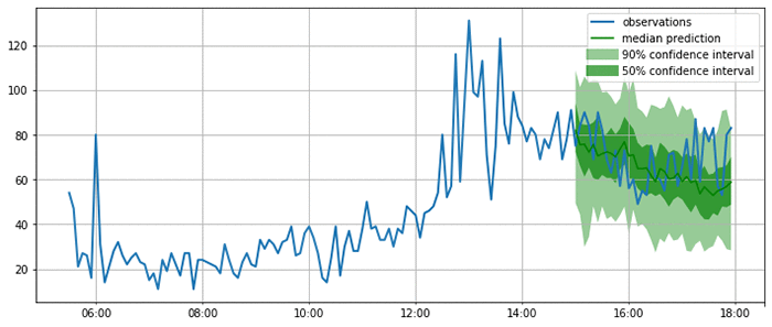
Now use the predictor to plot the model’s forecasts on a few time ranges that start after the last time point seen during training. This is useful for getting a qualitative feel for the quality of the outputs produced by this model.

Using the same base dataset as before, create a few test instances by taking data past the time range previously used for training.

test_data = ListDataset(
    [
        {"start": df.index[0], "target": df.value[:"2015-04-10 03:00:00"]},
        {"start": df.index[0], "target": df.value[:"2015-04-15 18:00:00"]},
        {"start": df.index[0], "target": df.value[:"2015-04-20 12:00:00"]}
    ],
    freq = "5min"
)

As you can see from the following plots, the model produces probabilistic predictions. This is important because it provides an estimate of how confident the model is, and allows downstream decisions based on these forecasts to account for this uncertainty.

from itertools import islice
from gluonts.evaluation.backtest import make_evaluation_predictions

def plot_forecasts(tss, forecasts, past_length, num_plots):
    for target, forecast in islice(zip(tss, forecasts), num_plots):
        ax = target[-past_length:].plot(figsize=(12, 5), linewidth=2)
        forecast.plot(color='g')
        plt.grid(which='both')
        plt.legend(["observations", "median prediction", "90% confidence interval", "50% confidence interval"])
        plt.show()

forecast_it, ts_it = make_evaluation_predictions(test_data, predictor=predictor, num_eval_samples=100)
forecasts = list(forecast_it)
tss = list(ts_it)
plot_forecasts(tss, forecasts, past_length=150, num_plots=3)

Now that you are satisfied that the forecasts look reasonable, you can compute a quantitative evaluation of the forecasts for all the time series in the test set using a variety of metrics. GluonTS provides an Evaluator component, which performs this model evaluation. It produces some commonly used error metrics such as MSE, MASE, symmetric MAPE, RMSE, and (weighted) quantile losses.

rom gluonts.evaluation import Evaluator

evaluator = Evaluator(quantiles=[0.5], seasonality=2016)

agg_metrics, item_metrics = evaluator(iter(tss), iter(forecasts), num_series=len(test_data))
agg_metrics

{'MSE': 163.59102376302084,
 'abs_error': 1090.9220886230469,
 'abs_target_sum': 5658.0,
 'abs_target_mean': 52.38888888888889,
 'seasonal_error': 18.833625618877182,
 'MASE': 0.5361500323952336,
 'sMAPE': 0.21201368270827592,
 'MSIS': 21.446000940010823,
 'QuantileLoss[0.5]': 1090.9221000671387,
 'Coverage[0.5]': 0.34259259259259256,
 'RMSE': 12.790270668090681,
 'NRMSE': 0.24414090352665138,
 'ND': 0.19281054942082837,
 'wQuantileLoss[0.5]': 0.19281055144346743,
 'mean_wQuantileLoss': 0.19281055144346743,
 'MAE_Coverage': 0.15740740740740744}

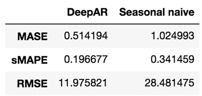
You can now compare these metrics against those produced by other models, or to the business requirements for your forecasting application. For example, you can produce forecasts using the seasonal naive method. This model assumes that the data has a fixed seasonality (in this case, 2016 time steps correspond to a week), and produces forecasts by copying past observations based on it.

from gluonts.model.seasonal_naive import SeasonalNaivePredictor

seasonal_predictor_1W = SeasonalNaivePredictor(freq="5min", prediction_length=36, season_length=2016)

forecast_it, ts_it = make_evaluation_predictions(test_data, predictor=seasonal_predictor_1W, num_eval_samples=100)
forecasts = list(forecast_it)
tss = list(ts_it)

agg_metrics_seasonal, item_metrics_seasonal = evaluator(iter(tss), iter(forecasts), num_series=len(test_data))

df_metrics = pd.DataFrame.join(
    pd.DataFrame.from_dict(agg_metrics, orient='index').rename(columns={0: "DeepAR"}),
    pd.DataFrame.from_dict(agg_metrics_seasonal, orient='index').rename(columns={0: "Seasonal naive"})
)
df_metrics.loc[["MASE", "sMAPE", "RMSE"]]

By looking at these metrics, you can get an idea of how your model compares to baselines or other advanced models. To improve the results, tweak the architecture or the hyperparameters.

Help make GluonTS better!

In this post, I only touched on a small subset of functionality provided by GluonTS. If you would like to dive deeper, I encourage you to check out tutorials and further examples.

GluonTS is open source under the Apache license. We welcome and encourage contributions from the community as bug reports and pull requests. Head over to the GluonTS GitHub repo now!

About the Authors

Jan Gasthaus is a Senior Machine Learning Scientist with AWS AI Labs where his passion is designing machine learning models, algorithms, and systems, and deploying them at scale.

Lorenzo Stella is an Applied Scientist on the AWS AI Labs team. His research interests are in machine learning and optimization. He has worked on probabilistic and deep models for forecasting.

Tim Januschowski is a Machine Learning Science Manager at AWS AI Labs. He has worked on forecasting and has produced end-to-end solutions for a wide variety of forecasting problems, from demand forecasting to server capacity forecasting over the course of his tenure at Amazon.

Richard Lee is a Product Manager at AWS AI Labs. He is passionate about how Artificial Intelligence impacts the worlds around us, and is on a mission to make it accessible to all. He is also a pilot, science and nature admirer, and beginner cook.

Syama Sundar Rangapuram is a Machine Learning Scientist at AWS AI Labs. His research interests are in machine learning and optimization. In forecasting, he has worked on probabilistic models and data-driven models in particular for the cold-start problem.

Konstantinos Benidis is an Applied Scientist at AWS AI Labs. His research interests are in machine learning, optimization and financial engineering. He has worked on probabilistic and deep models for forecasting.

Alexander Alexandrov is a Post-Doc on the AWS AI Labs team and TU-Berlin. He is passionate about scalable data management, data analytics applications, and optimizing DSLs. 

David Salinas is a Senior Applied Scientist in the AWS AI Labs team. He is working on applying deep-learning to various application such as forecasting or NLP.

Danielle Robinson is an Applied Scientist in the AWS AI Labs team. She is working on combining deep learning methods with classical statiscal methods for forecasting. Her interests also include numerical linear algebra, numerical optimization and numerical PDEs.

Yuyang (Bernie) Wang is a Senior Machine Learning Scientist in Amazon AI Labs, working mainly on large-scale probabilistic machine learning with its application in Forecasting. His research interests span statistical machine learning, numerical linear algebra, and random matrix theory. In forecasting, Yuyang has worked on all aspects ranging from practical applications to theoretical foundations.

Valentin Flunkert is a Senior Machine Learning Scientist at AWS AI Labs. He is passionate about building machine learning systems for solving business problems. He has worked on a variety of machine learning and forecasting problems at Amazon. 

Michael Bohlke-Schneider is a Data Scientist in AWS AI Labs/Fulfillment Technology, researching and developing forecasting algorithms in SageMaker and applying forecasting to business problems.

Jasper Schulz is a software development engineer in the AWS AI Labs team.

If you’ve ever competed in a sporting event and painstakingly sifted through event photos to find yourself later, you’ll appreciate GeoSnapShot’s innovative solution powered by Amazon Rekognition.

GeoSnapShot founder Andy Edwards was first introduced to the world of sports photography when he started accompanying his wife, a competitive equestrian, to her riding events and photographing her and her friends.While he enjoyed taking great photos of everyone, he was frustrated by the manual, time-intensive process required post-event to identify each rider and distribute the photos to them. He noticed many other photographers in the same situation, and the sad consequence was a loss of the special memories they captured simply because the sorting process was too hard.

Setting out to solve this challenge – and indeed, multiple related challenges for photographers and sports organizations worldwide – Andy started GeoSnapShot in 2013. The company partners with event organizers to enable any athlete who opts in and uploads a selfie to find images of themselves quickly and easily. It does this by using Amazon Rekognition in two ways: for direct comparisons of users’ selfies to the photos from an event, and for optical character recognition to identify their competition bib numbers. With those inputs, GeoSnapShot is able to process thousands of event photos in near real-time, expediting an effort that used to require event organizers to spend many hours manually matching bib numbers to athlete names and sorting the photos by athlete.

This heavy lifting meant that athletes used to wait days or weeks for their photos to be available. Now, GeoSnapShot’s unique solution for sports photography makes it possible for athletes to start reviewing their photos before the sweat has even dried. As a result, photography sales for event organizers have increased by almost 30 percent, and customer satisfaction has increased substantially.

GeoSnapShot’s solutions are being used across 92 countries, where amateur photographers and professionals alike laud the user-friendly solution built on AWS. Perhaps the truest testimony of the power of the technology is that the popular global endurance event company Tough Mudder recently started using GeoSnapShot. Tough Mudder participants are often barely recognizable due to the unavoidable head-toe coating of mud inherent to the competition, and yet GeoSnapShot’s participant identification is successful. (No, competitors don’t need to upload a mud-covered selfie for it to work either; a more glamorous image works fine too!)

Tough Mudder’s VP of Live Events, Johnny Little, comments, “Reliving the memories made is vital to our participants and GeoSnapShot have an outstanding global photography platform that provides the best solution for every Tough Mudder event worldwide.”

Andy lauds AWS AI as the underpinning of that solution. “AWS provided us with the most flexible technology platform as we started building our business. As GeoSnapShot is a platform, it’s important we use leading technology to deliver the very best experience for all our customers. AWS continues to provide us with a world-leading technology. We are delighted with the access we have to the technology and business teams to drive future solutions.”

GeoSnapShot has chosen AWS as their primary AI/ML platform, and the company’s tech stack will get even deeper in the coming months, as the company is currently in the process of implementing a video solution in addition to the still photos. GeoSnapShot believes that providing athletes with memories of their achievements in stills and video, all using recognition technology, is the future of sports media.

Ultimately, GeoSnapShot wants every event and every photographer globally to have the opportunity to use its platform. Andy comments, “After all, memories of our lives and those of our loved ones are very precious and should be captured.”

To learn more about Amazon Rekognition, visit https://aws.amazon.com/rekognition/.

About the Author

Marisa Messina is on the AWS AI marketing team, where her job includes identifying the most innovative AWS-using customers and showcasing their inspiring stories. Prior to AWS, she worked on consumer-facing hardware and then university-facing cloud offerings at Microsoft. Outside of work, she enjoys exploring the Pacific Northwest hiking trails, cooking without recipes, and dancing in the rain.

Documents are a primary tool for record keeping, communication, collaboration, and transactions across many industries, including financial, medical, legal, and real estate. The millions of mortgage applications and hundreds of millions of W2 tax forms processed each year are just a few examples of such documents. A lot of information is locked in unstructured documents. It usually requires time-consuming and complex processes to enable search and discovery, business process automation, and compliance control for these documents.

In this post, I show how you can take advantage of Amazon Textract to automatically extract text and data from scanned documents without any machine learning (ML) experience. While AWS takes care of building, training, and deploying advanced ML models in a highly available and scalable environment, you take advantage of these models with simple-to-use API actions. Here are the use cases that I cover in this post:

• Text detection from documents
• Multi-column detection and reading order
• Natural language processing and document classification
• Natural language processing for medical documents
• Document translation
• Search and discovery
• Form extraction and processing
• Compliance control with document redaction
• Table extraction and processing
• PDF document processing

Amazon Textract

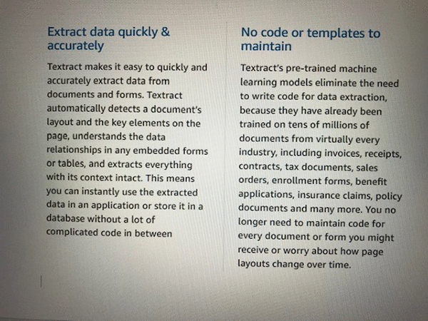
Before I get started with the use cases, let me review and introduce some of the core features. Amazon Textract goes beyond simple optical character recognition (OCR) to also identify the contents of fields in forms and information stored in tables. This allows you to use Amazon Textract to instantly “read” virtually any type of document and accurately extract text and data without the need for any manual effort or custom code.

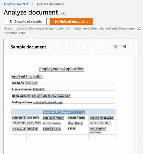
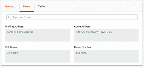
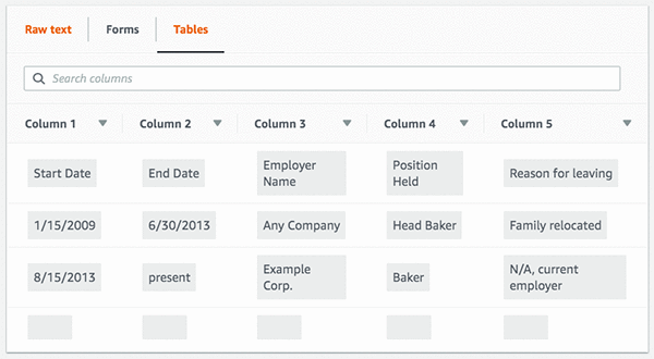
The following images show an example document and corresponding extracted text, form, and table data using Amazon Textract in the AWS Management Console.

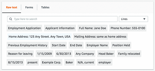
The following image shows the lines extracted as raw text from the document.

The following image shows the extracted form fields and their corresponding values.

The following image shows the extracted table, cells, and the text in those cells.

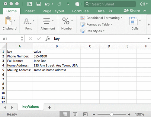
To quickly download a zip file containing the output, choose Download results. You can choose various formats, including raw JSON, text, and CSV files for forms and tables.

In addition to the detected content, Amazon Textract provides additional information, like confidence scores and bounded boxes for detected elements. It gives you control on how you consume extracted content and integrate it into various business applications.

Amazon Textract provides both synchronous and asynchronous API actions to extract document text and analyze the document text data. Synchronous APIs can be used for single-page documents and low latency use cases such as mobile capture. Asynchronous APIs can be used for multi-page documents such as PDF documents with thousands of pages. For more information, see the Amazon Textract API Reference.

Use cases

Now, write some code to take advantage of Amazon Textract API operations using the AWS SDK and see how easy it is to build power-smart applications. I will also use the JSON Parser Library for some of the below use cases.

Text detection from documents

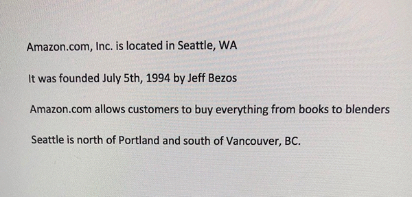
I start with a simple example on how to detect text from a document. Use the following image as an input document to Amazon Textract. As you can see, the sample image is not of good quality, but Amazon Textract can still detect the text with accuracy.

The following code example shows how to use a few lines of code to send this sample image to Amazon Textract and get a JSON response back. You then iterate over the blocks in JSON and print the detected text, as shown below.

import boto3

# Document
s3BucketName = "ki-textract-demo-docs"
documentName = "simple-document-image.jpg"

# Amazon Textract client
textract = boto3.client('textract')

# Call Amazon Textract
response = textract.detect_document_text(
    Document={
        'S3Object': {
            'Bucket': s3BucketName,
            'Name': documentName
        }
    })

#print(response)

# Print detected text
for item in response["Blocks"]:
    if item["BlockType"] == "LINE":
        print ('33[94m' +  item["Text"] + '33[0m')

The following JSON response is what you receive from Amazon Textract, with blocks representing detected text in the document.

{
    "Blocks": [
        {
            "Geometry": {
                "BoundingBox": {
                    "Width": 1.0, 
                    "Top": 0.0, 
                    "Left": 0.0, 
                    "Height": 1.0
                }, 
                "Polygon": [
                    {
                        "Y": 0.0, 
                        "X": 0.0
                    }, 
                    {
                        "Y": 0.0, 
                        "X": 1.0
                    }, 
                    {
                        "Y": 1.0, 
                        "X": 1.0
                    }, 
                    {
                        "Y": 1.0, 
                        "X": 0.0
                    }
                ]
            }, 
            "Relationships": [
                {
                    "Type": "CHILD", 
                    "Ids": [
                        "2602b0a6-20e3-4e6e-9e46-3be57fd0844b", 
                        "82aedd57-187f-43dd-9eb1-4f312ca30042", 
                        "52be1777-53f7-42f6-a7cf-6d09bdc15a30", 
                        "7ca7caa6-00ef-4cda-b1aa-5571dfed1a7c"
                    ]
                }
            ], 
            "BlockType": "PAGE", 
            "Id": "8136b2dc-37c1-4300-a9da-6ed8b276ea97"
        }..... 
        
    ], 
    "DocumentMetadata": {
        "Pages": 1
    }
}

The following image shows the output of the detected text.

Multi-column detection and reading order

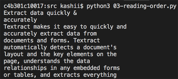
Traditional OCR solutions read left to right, do not detect multiple columns, and end up generating incorrect reading order for multi-column documents. In addition to detecting text, Amazon Textract provides additional geometry information that can be used to detect multiple columns and print the text in reading order.

The following image is a two-column document. Similar to the earlier example, the image is not good quality but Amazon Textract still performs well.

The following example code shows processing the document with Amazon Textract and taking advantage of geometry information to print the text in reading order.

import boto3

# Document
s3BucketName = "ki-textract-demo-docs"
documentName = "two-column-image.jpg"

# Amazon Textract client
textract = boto3.client('textract')

# Call Amazon Textract
response = textract.detect_document_text(
    Document={
        'S3Object': {
            'Bucket': s3BucketName,
            'Name': documentName
        }
    })

#print(response)

# Detect columns and print lines
columns = []
lines = []
for item in response["Blocks"]:
      if item["BlockType"] == "LINE":
        column_found=False
        for index, column in enumerate(columns):
            bbox_left = item["Geometry"]["BoundingBox"]["Left"]
            bbox_right = item["Geometry"]["BoundingBox"]["Left"] + item["Geometry"]["BoundingBox"]["Width"]
            bbox_centre = item["Geometry"]["BoundingBox"]["Left"] + item["Geometry"]["BoundingBox"]["Width"]/2
            column_centre = column['left'] + column['right']/2

            if (bbox_centre > column['left'] and bbox_centre < column['right']) or (column_centre > bbox_left and column_centre < bbox_right):
                #Bbox appears inside the column
                lines.append([index, item["Text"]])
                column_found=True
                break
        if not column_found:
            columns.append({'left':item["Geometry"]["BoundingBox"]["Left"], 'right':item["Geometry"]["BoundingBox"]["Left"] + item["Geometry"]["BoundingBox"]["Width"]})
            lines.append([len(columns)-1, item["Text"]])

lines.sort(key=lambda x: x[0])
for line in lines:
    print (line[1])

The following image shows the output of the detected text in the correct reading order.

Natural language processing and document classification

Customer emails, support tickets, product reviews, social media, even advertising copy all represent insights into customer sentiment that can be put to work for your business. A lot of such content contains images or scanned versions of documents. After text is extracted from these documents, you can use Amazon Comprehend to detect sentiment, entities, key phrases, syntax and topics. You can also train Amazon Comprehend to detect custom entities based on your business domain. These insights can then be used to classify documents, automate business process workflows, and ensure compliance.

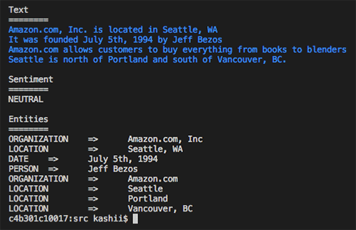
The following example code shows processing the first image sample used earlier with Amazon Textract to extract text and then using Amazon Comprehend to detect sentiment and entities.

import boto3

# Document
s3BucketName = "ki-textract-demo-docs"
documentName = "simple-document-image.jpg"

# Amazon Textract client
textract = boto3.client('textract')

# Call Amazon Textract
response = textract.detect_document_text(
    Document={
        'S3Object': {
            'Bucket': s3BucketName,
            'Name': documentName
        }
    })

#print(response)

# Print text
print("nTextn========")
text = ""
for item in response["Blocks"]:
    if item["BlockType"] == "LINE":
        print ('33[94m' +  item["Text"] + '33[0m')
        text = text + " " + item["Text"]

# Amazon Comprehend client
comprehend = boto3.client('comprehend')

# Detect sentiment
sentiment =  comprehend.detect_sentiment(LanguageCode="en", Text=text)
print ("nSentimentn========n{}".format(sentiment.get('Sentiment')))

# Detect entities
entities =  comprehend.detect_entities(LanguageCode="en", Text=text)
print("nEntitiesn========")
for entity in entities["Entities"]:
    print ("{}t=>t{}".format(entity["Type"], entity["Text"]))

The following image shows the output text along with the text analysis from Amazon Comprehend. You can see that it found the sentiment to be “Neutral” and detected “Amazon” as an organization, “Seattle, WA” as a location and “July 5th, 1994” as a date, along with other entities.

Natural language processing for medical documents

One of the important ways to improve patient care and accelerate clinical research is by understanding and analyzing the insights and relationships that are “trapped” in free-form medical text. These can include hospital admission notes and a patient’s medical history.

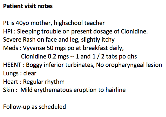
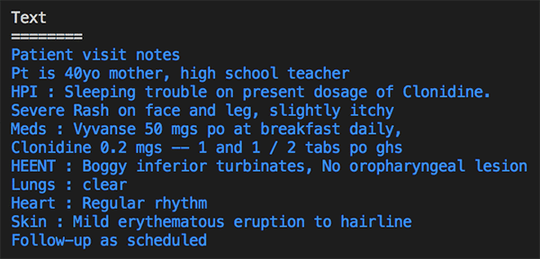
In this example, use the following document to extract text using Amazon Textract. You then use Amazon Comprehend Medical to extract medical entities, such as medical condition, medication, dosage, strength, and protected health information (PHI).

The following example code shows how different medical entities are detected.

import boto3

# Document
s3BucketName = "ki-textract-demo-docs"
documentName = "medical-notes.png"

# Amazon Textract client
textract = boto3.client('textract')

# Call Amazon Textract
response = textract.detect_document_text(
    Document={
        'S3Object': {
            'Bucket': s3BucketName,
            'Name': documentName
        }
    })

#print(response)

# Print text
print("nTextn========")
text = ""
for item in response["Blocks"]:
    if item["BlockType"] == "LINE":
        print ('33[94m' +  item["Text"] + '33[0m')
        text = text + " " + item["Text"]

# Amazon Comprehend client
comprehend = boto3.client('comprehendmedical')

# Detect medical entities
entities =  comprehend.detect_entities(Text=text)
print("nMidical Entitiesn========")
for entity in entities["Entities"]:
    print("- {}".format(entity["Text"]))
    print ("   Type: {}".format(entity["Type"]))
    print ("   Category: {}".format(entity["Category"]))
    if(entity["Traits"]):
        print("   Traits:")
        for trait in entity["Traits"]:
            print ("    - {}".format(trait["Name"]))
    print("n")

The following image and text block shows the output of the detected text with information categorized by type. It detected “40yo” as the age with category “Protected Health Information”. It also detected different medical conditions, including sleeping trouble, rash, inferior turbinates, erythematous eruption, and others. It recognized different medications and anatomy information.

Medical Entities
========
- 40yo
   Type: AGE
   Category: PROTECTED_HEALTH_INFORMATION
- Sleeping trouble
   Type: DX_NAME
   Category: MEDICAL_CONDITION
   Traits:
    - SYMPTOM
- Clonidine
   Type: GENERIC_NAME
   Category: MEDICATION
- Rash
   Type: DX_NAME
   Category: MEDICAL_CONDITION
   Traits:
    - SYMPTOM
- face
   Type: SYSTEM_ORGAN_SITE
   Category: ANATOMY
- leg
   Type: SYSTEM_ORGAN_SITE
   Category: ANATOMY
- Vyvanse
   Type: BRAND_NAME
   Category: MEDICATION
- Clonidine
   Type: GENERIC_NAME
   Category: MEDICATION
- HEENT
   Type: SYSTEM_ORGAN_SITE
   Category: ANATOMY
- Boggy inferior turbinates
   Type: DX_NAME
   Category: MEDICAL_CONDITION
   Traits:
    - SIGN
- inferior
   Type: DIRECTION
   Category: ANATOMY
- turbinates
   Type: SYSTEM_ORGAN_SITE
   Category: ANATOMY
- oropharyngeal lesion
   Type: DX_NAME
   Category: MEDICAL_CONDITION
   Traits:
    - SIGN
    - NEGATION
- Lungs
   Type: SYSTEM_ORGAN_SITE
   Category: ANATOMY
- clear Heart
   Type: DX_NAME
   Category: MEDICAL_CONDITION
   Traits:
    - SIGN
- Heart
   Type: SYSTEM_ORGAN_SITE
   Category: ANATOMY
- Regular rhythm
   Type: DX_NAME
   Category: MEDICAL_CONDITION
   Traits:
    - SIGN
- Skin
   Type: SYSTEM_ORGAN_SITE
   Category: ANATOMY
- erythematous eruption
   Type: DX_NAME
   Category: MEDICAL_CONDITION
   Traits:
    - SIGN
- hairline
   Type: SYSTEM_ORGAN_SITE
   Category: ANATOMY

Document translation

Many organizations localize content for international users, such as websites and applications. They must translate large volumes of documents efficiently. You can use Amazon Textract along with Amazon Translate to extract text and data and then translate them into other languages.

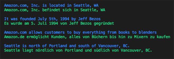
The following code example shows translating the text in the first image to German.

import boto3

# Document
s3BucketName = "ki-textract-demo-docs"
documentName = "simple-document-image.jpg"

# Amazon Textract client
textract = boto3.client('textract')

# Call Amazon Textract
response = textract.detect_document_text(
    Document={
        'S3Object': {
            'Bucket': s3BucketName,
            'Name': documentName
        }
    })

#print(response)

# Amazon Translate client
translate = boto3.client('translate')

print ('')
for item in response["Blocks"]:
    if item["BlockType"] == "LINE":
        print ('33[94m' +  item["Text"] + '33[0m')
        result = translate.translate_text(Text=item["Text"], SourceLanguageCode="en", TargetLanguageCode="de")
        print ('33[92m' + result.get('TranslatedText') + '33[0m')
    print ('')

The following image shows the output of the detected text, translated to German line by line.

Search and discovery

Extracting structured data from documents and creating a smart index using Amazon Elasticsearch Service (Amazon ES) allows you to search through millions of documents quickly. For example, a mortgage company could use Amazon Textract to process millions of scanned loan applications in a matter of hours and have the extracted data indexed in Amazon ES. This would allow them to create search experiences like searching for loan applications where the applicant name is John Doe, or searching for contracts where the interest rate is 2 percent.

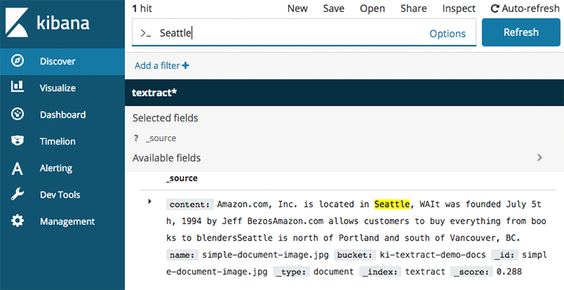
The following code example shows how you can extract text from the first image, store it in Amazon ES, and then search it using Kibana. You can also build a custom UI experience by taking advantage of the Amazon ES APIs. Later in the post, as you learn how to extract forms and tables, that structured data can then be indexed similarly to enable smart search.

import boto3
from elasticsearch import Elasticsearch, RequestsHttpConnection
from requests_aws4auth import AWS4Auth

def indexDocument(bucketName, objectName, text):

    # Update host with endpoint of your Elasticsearch cluster
    #host = "search--xxxxxxxxxxxxxx.us-east-1.es.amazonaws.com
    host = "searchxxxxxxxxxxxxxxxx.us-east-1.es.amazonaws.com"
    region = 'us-east-1'

    if(text):
        service = 'es'
        ss = boto3.Session()
        credentials = ss.get_credentials()
        region = ss.region_name

        awsauth = AWS4Auth(credentials.access_key, credentials.secret_key, region, service, session_token=credentials.token)

        es = Elasticsearch(
            hosts = [{'host': host, 'port': 443}],
            http_auth = awsauth,
            use_ssl = True,
            verify_certs = True,
            connection_class = RequestsHttpConnection
        )

        document = {
            "name": "{}".format(objectName),
            "bucket" : "{}".format(bucketName),
            "content" : text
        }

        es.index(index="textract", doc_type="document", id=objectName, body=document)

        print("Indexed document: {}".format(objectName))

# Document
s3BucketName = "ki-textract-demo-docs"
documentName = "simple-document-image.jpg"

# Amazon Textract client
textract = boto3.client('textract')

# Call Amazon Textract
response = textract.detect_document_text(
    Document={
        'S3Object': {
            'Bucket': s3BucketName,
            'Name': documentName
        }
    })

#print(response)

# Print detected text
text = ""
for item in response["Blocks"]:
    if item["BlockType"] == "LINE":
        print ('33[94m' +  item["Text"] + '33[0m')
        text += item["Text"]

indexDocument(s3BucketName, documentName, text)

# You can view index documents in Kibana Dashboard

The following image shows the output of extracted text in Kibana search results.

Form extraction and processing

Amazon Textract can provide the inputs required to automatically process forms without human intervention. For example, a bank could write code to read PDFs of loan applications. The information contained in the document could be used to initiate all of the necessary background and credit checks to approve the loan so that customers can get instant results for their application rather than having to wait several days for manual review and validation.

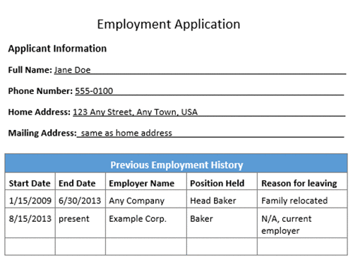
The following image is an employment application with form fields and a table.

The following code example shows how to extract forms from the employment application and process different fields.

import boto3
from trp import Document

# Document
s3BucketName = "ki-textract-demo-docs"
documentName = "employmentapp.png"

# Amazon Textract client
textract = boto3.client('textract')

# Call Amazon Textract
response = textract.analyze_document(
    Document={
        'S3Object': {
            'Bucket': s3BucketName,
            'Name': documentName
        }
    },
    FeatureTypes=["FORMS"])

#print(response)

doc = Document(response)

for page in doc.pages:
    # Print fields
    print("Fields:")
    for field in page.form.fields:
        print("Key: {}, Value: {}".format(field.key, field.value))

    # Get field by key
    print("nGet Field by Key:")
    key = "Phone Number:"
    field = page.form.getFieldByKey(key)
    if(field):
        print("Key: {}, Value: {}".format(field.key, field.value))

    # Search fields by key
    print("nSearch Fields:")
    key = "address"
    fields = page.form.searchFieldsByKey(key)
    for field in fields:
        print("Key: {}, Value: {}".format(field.key, field.value))

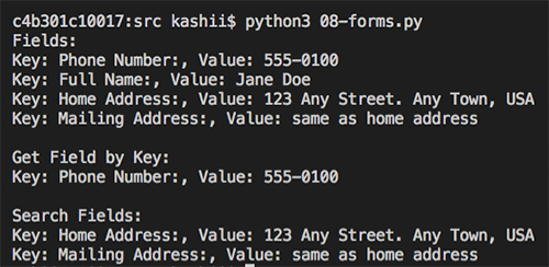
The following image is the output of detected form for the employment application.

Compliance control with document redaction

Because Amazon Textract identifies data types and form labels automatically, AWS helps secure infrastructure so that you can maintain compliance with information controls. For example, an insurer could use Amazon Textract to feed a workflow that automatically redacts personally identifiable information (PII) for review before archiving claim forms. Amazon Textract recognizes the important fields that require protection.

The following code example shows extracting all the form fields in the employment application used earlier, and then redacting all the address fields.

import boto3
from trp import Document
from PIL import Image, ImageDraw

# Document
s3BucketName = "ki-textract-demo-docs"
documentName = "employmentapp.png"

# Amazon Textract client
textract = boto3.client('textract')

# Call Amazon Textract
response = textract.analyze_document(
    Document={
        'S3Object': {
            'Bucket': s3BucketName,
            'Name': documentName
        }
    },
    FeatureTypes=["FORMS"])

#print(response)

doc = Document(response)

# Redact document
img = Image.open(documentName)

width, height = img.size

if(doc.pages):
    page = doc.pages[0]
    for field in page.form.fields:
        if(field.key and field.value and "address" in field.key.text.lower()):
        #if(field.key and field.value):
            print("Redacting => Key: {}, Value: {}".format(field.key.text, field.value.text))
            
            x1 = field.value.geometry.boundingBox.left*width
            y1 = field.value.geometry.boundingBox.top*height-2
            x2 = x1 + (field.value.geometry.boundingBox.width*width)+5
            y2 = y1 + (field.value.geometry.boundingBox.height*height)+2

            draw = ImageDraw.Draw(img)
            draw.rectangle([x1, y1, x2, y2], fill="Black")

img.save("redacted-{}".format(documentName))

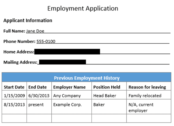
The following image is the output redacted version of employment application.

Table extraction and processing

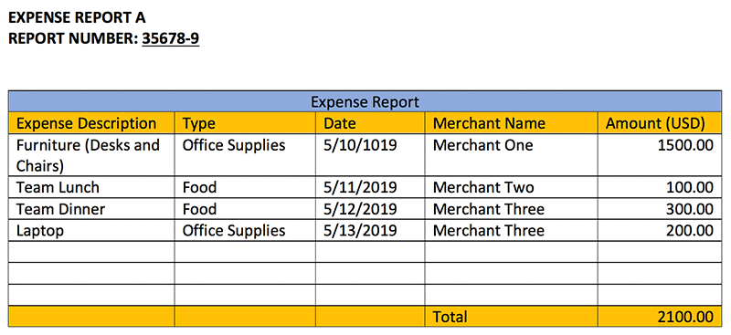
Amazon Textract can detect tables and their content. A company can extract all the amounts from an expense report and apply rules, such as any expense more than $1000 needs extra review.

The following code example uses the expense report sample document and prints the content of each cell, along with a warning message if any expense is more than $1000.

import boto3
from trp import Document

# Document
s3BucketName = "ki-textract-demo-docs"
documentName = "expense.png"

# Amazon Textract client
textract = boto3.client('textract')

# Call Amazon Textract
response = textract.analyze_document(
    Document={
        'S3Object': {
            'Bucket': s3BucketName,
            'Name': documentName
        }
    },
    FeatureTypes=["TABLES"])

#print(response)

doc = Document(response)

def isFloat(input):
  try:
    float(input)
  except ValueError:
    return False
  return True

warning = ""
for page in doc.pages:
     # Print tables
    for table in page.tables:
        for r, row in enumerate(table.rows):
            itemName  = ""
            for c, cell in enumerate(row.cells):
                print("Table[{}][{}] = {}".format(r, c, cell.text))
                if(c == 0):
                    itemName = cell.text
                elif(c == 4 and isFloat(cell.text)):
                    value = float(cell.text)
                    if(value > 1000):
                        warning += "{} is greater than $1000.".format(itemName)
if(warning):
    print("nReview needed:n====================n" + warning)

The following text is the output of the table cells and the text within.

Table[0][0] = Expense Description 
Table[0][1] = Type 
Table[0][2] = Date 
Table[0][3] = Merchant Name 
Table[0][4] = Amount (USD) 
Table[1][0] = Furniture (Desks and Chairs) 
Table[1][1] = Office Supplies 
Table[1][2] = 5/10/1019 
Table[1][3] = Merchant One 
Table[1][4] = 1500.00 
Table[2][0] = Team Lunch 
Table[2][1] = Food 
Table[2][2] = 5/11/2019 
Table[2][3] = Merchant Two 
Table[2][4] = 100.00 
Table[3][0] = Team Dinner 
Table[3][1] = Food 
Table[3][2] = 5/12/2019 
Table[3][3] = Merchant Three 
Table[3][4] = 300.00 
Table[4][0] = Laptop 
Table[4][1] = Office Supplies 
Table[4][2] = 5/13/2019 
Table[4][3] = Merchant Three 
Table[4][4] = 200.00 
Table[5][0] = 
Table[5][1] = 
Table[5][2] = 
Table[5][3] = 
Table[5][4] = 
Table[6][0] = 
Table[6][1] = 
Table[6][2] = 
Table[6][3] = 
Table[6][4] = 
Table[7][0] = 
Table[7][1] = 
Table[7][2] = 
Table[7][3] = 
Table[7][4] = 
Table[8][0] = 
Table[8][1] = 
Table[8][2] = 
Table[8][3] = Total 
Table[8][4] = 2100.00 

Review needed:
====================
Furniture (Desks and Chairs) is greater than $1000.

PDF document processing (async API operations)

For the earlier examples, you used images with the sync API operations. Now, see how you can process PDF files using the async API operations.

First, use StartDocumentTextDetection or StartDocumentAnalysis to start an Amazon Textract job. As the job completes, Amazon Textract publishes the results of an Amazon Textract request, including completion status, to Amazon SNS. You can then use GetDocumentTextDetection or GetDocumentAnalysis to get the results from Amazon Textract.

The following code example shows how to start a job, get job status, and then process the results. Click here for the sample PDF document. For more information, see Calling Amazon Textract Asynchronous Operations.

import boto3
import time

def startJob(s3BucketName, objectName):
    response = None
    client = boto3.client('textract')
    response = client.start_document_text_detection(
    DocumentLocation={
        'S3Object': {
            'Bucket': s3BucketName,
            'Name': objectName
        }
    })

    return response["JobId"]

def isJobComplete(jobId):
    # For production use cases, use SNS based notification 
    # Details at: https://docs.aws.amazon.com/textract/latest/dg/api-async.html
    time.sleep(5)
    client = boto3.client('textract')
    response = client.get_document_text_detection(JobId=jobId)
    status = response["JobStatus"]
    print("Job status: {}".format(status))

    while(status == "IN_PROGRESS"):
        time.sleep(5)
        response = client.get_document_text_detection(JobId=jobId)
        status = response["JobStatus"]
        print("Job status: {}".format(status))

    return status

def getJobResults(jobId):

    pages = []

    client = boto3.client('textract')
    response = client.get_document_text_detection(JobId=jobId)
    
    pages.append(response)
    print("Resultset page recieved: {}".format(len(pages)))
    nextToken = None
    if('NextToken' in response):
        nextToken = response['NextToken']

    while(nextToken):

        response = client.get_document_text_detection(JobId=jobId, NextToken=nextToken)

        pages.append(response)
        print("Resultset page recieved: {}".format(len(pages)))
        nextToken = None
        if('NextToken' in response):
            nextToken = response['NextToken']

    return pages

# Document
s3BucketName = "ki-textract-demo-docs"
documentName = "Amazon-Textract-Pdf.pdf"

jobId = startJob(s3BucketName, documentName)
print("Started job with id: {}".format(jobId))
if(isJobComplete(jobId)):
    response = getJobResults(jobId)

#print(response)

# Print detected text
for resultPage in response:
    for item in resultPage["Blocks"]:
        if item["BlockType"] == "LINE":
            print ('33[94m' +  item["Text"] + '33[0m')

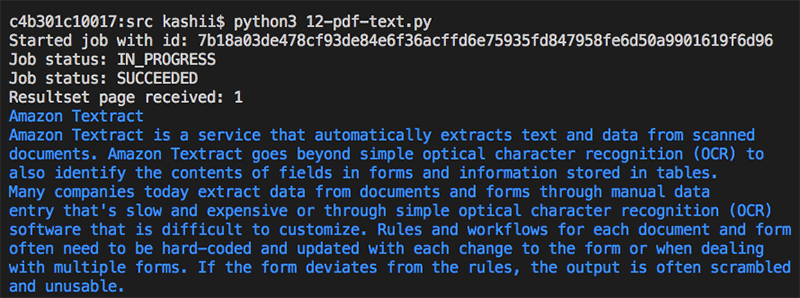
The following image shows the job status as the API call proceeds.

Conclusion

In this post, I showed you how to use Amazon Textract to automatically extract text and data from scanned documents without any machine learning (ML) experience. I covered use cases in fields such as finance, healthcare, and HR, but there are many other opportunities where the ability to unlock text and data from unstructured documents could be most useful. To learn more about Amazon Textract, read about processing single-page and multi-page documents, working with block objects, and code samples.

You can start using Amazon Textract in US East (N. Virginia), US East (Ohio), US West (Oregon), and EU (Ireland) today.

About the Authors

Kashif Imran is a Solutions Architect at Amazon Web Services. He works with some of the largest strategic AWS customers to provide technical guidance and design advice. His expertise spans application architecture, serverless, containers, NoSQL and machine learning.

This is a guest post by Evan Harris, Manager of Machine Learning at Ibotta. In their own words, “Ibotta is transforming the shopping experience by making it easy for consumers to earn cash back on everyday purchases through a single smartphone app. The company partners with leading brands and retailers to offer offers on groceries, electronics, clothing, gifts, home and office supplies, restaurant dining, and more.”

The technical divisions within high-growth, mid-stage companies are prone to a unique set of challenges.  High on the list for many such companies is building quality applications quickly and effectively.

On the machine learning (ML) team at Ibotta—a mobile app that offers cash back on everyday purchases for millions of users—we have done a good deal of thinking and experimentation on this topic.  I would like to share how we leverage AWS to achieve core functionality, such as search with Amazon SageMaker.

In this post, I discuss the architecture of Ibotta’s search engine and how we use Amazon SageMaker with other AWS services to integrate real-time ML into the search experience of our mobile application. I hope that this post can shorten your search for a feasible solution to the comparable challenges in your organization, no matter the organization size.

Creating a streamlined mobile app experience, complete with a comprehensive and user-friendly search flow, is crucial for our business. Customers searching for deals before shopping must find useful content quickly or they’re liable to give up.

With a dedicated team of search relevancy engineers, ML engineers, designers, and mobile developers, we use as much modern technology as possible to rapidly develop and test new, creative improvements to our search relevancy. We prioritize the use of ML to inject data-driven intelligence into our search engine, pushing us beyond traditional information retrieval techniques.

Foundational search infrastructure

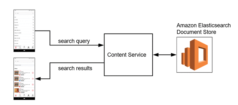
Our core infrastructure for search at Ibotta rests on our app’s array of microservices. Indexed documents live in Amazon Elasticsearch Service, which contains all of the content available to the mobile client at a given point in time. An internal content service talks to this document store on request and provides additional rules-based filtering functionality to ensure that only content available to the user making the request is returned.

The content service can receive input search queries and respond with relevant content, taking other contextual considerations into account. The service uses textbook lucene-style search relevancy techniques to retrieve appropriate content in the Elasticsearch document store.

ML-enhanced search infrastructure

The foundational search infrastructure leaves substantial room for improvement. Ibotta’s search problem space has unique challenges, particularly revolving content. One week, there might be an offer for certain brands in the app and another week they are gone. This is driven by the retailers with whom we partner, as they often want to promote an item only for a limited time.

Additionally, some brands and product categories are not available in the app at all, as we have yet to work with those retailers. We still want to show related content to users when their search queries don’t match exact content in the app. For example, a search for a non-carried brand of coffee should return other coffee brands that match across important attributes (flavor, size, price, etc.).

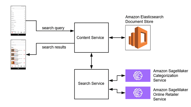
The solution here is query expansion. This is a common search technique that takes the user’s search query and adds context to it before querying the data store. In one case, we can add value by categorizing the search query in real time, enhancing the content retrieval and sorting algorithm. In other cases, after categorization, we’d like to look up and sort online retailers that specialize in the predicted category and return those as suggestions to the user.

To make these category inferences on-demand in real time, we use Amazon SageMaker. We can easily train models and deploy them as fully managed REST APIs to which internal microservices can make requests. An example request and response looks something like the following code:

{
    "term": "organic prepared horseradish"
}

{
    "categories": [
        "Condiments, Sauces & Seasonings",    
        "Sauces"
    ],
    "score": 0.901242
}

We use BlazingText, an algorithm built in to Amazon SageMaker. The supervised version of BlazingText is a powerful, flexible, and easy to use text classification model. Out of the box, we get scalable distributed training, Bayesian hyperparameter optimization, and real-time inference endpoint deployment. We’ve spent substantial time training and deploying our own text classification models for other use cases. We found a lot to like using the built-in Amazon SageMaker model and managed training and deployment service.

In one view, below is the architecture of our ML-enhanced search services architecture. As you’ll see, the querying and retrieval mechanism described above (and captured here as well) is complemented by SageMaker, which provides two distinct value-adds. First, it enables us to categorize the search query to deliver more relevant results, and second, it enables us to provide online retailers whose offerings are relevant to the query.

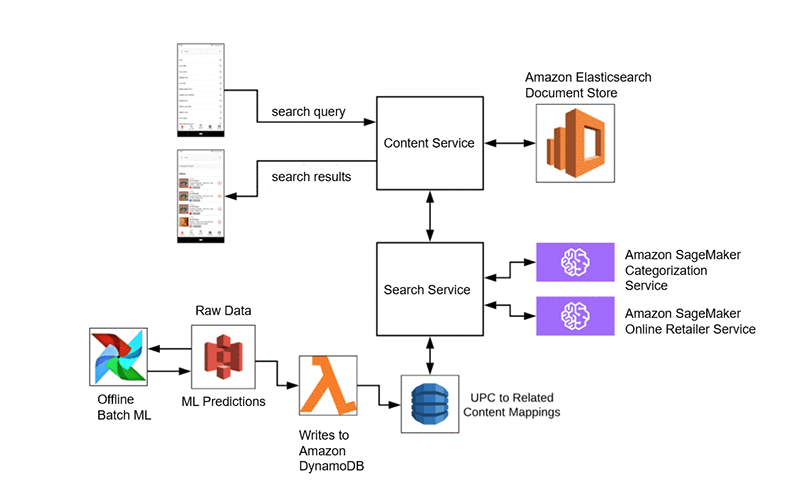
An additional ML value-add is our UPC barcode scan feature. Users can scan barcodes of consumer products with our app. If purchasing that UPC satisfies an offer, we return exact matches. If there isn’t an exact match, we use an unsupervised text similarity algorithm to find related offers to suggest to the user. If they can get cash back with our app, perhaps they will consider an alternative to the product that they scanned.

With the UPC feature, we know upfront the universe of UPCs for which we potentially have a similarity suggestion. Predictions can be made offline and written to an online data store, from which our services can make low-latency requests in real time. We use a combination of Amazon S3, AWS Lambda, Apache Airflow, and Amazon DynamoDB for this process. We see that addition to our architecture in the following diagram, in which the UPC input becomes a search query against which we execute.

We then get a mix of on-demand and batch ML models used as needed to enhance our search experience. With a broad services toolset, we are able to select the right tool for the job. Our production environment consists of fully managed AWS services, including offline data storage, online data storage, data transfer, and ML services.

Building to scale

When technologists talk about building to scale, they are often referring to horizontal scalability—perhaps something like Amazon S3 for storage or managed Kubernetes for compute. With these services, horizontal scaling is effectively infinite.

However, it’s often also useful to talk about scalability in terms of our ability to add new functionality to our services without overcomplicating any individual service or code base. Using microservices built on top of AWS, we are able to add or upgrade features while imposing minimal risk to the existing ecosystem.

We are also able to compartmentalize ownership, particularly allowing ML engineers to own their own services end-to-end. As long as the API contract doesn’t change, the ML team can iterate on their models independent of any contact with the owners of dependent services. Amazon SageMaker enables developers with basic Python skills and ML knowledge to support production microservices that integrate directly into our stack.

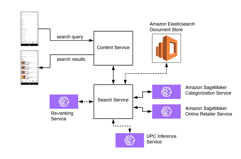
This sets us up for future iterations of our search service architecture that don’t require substantial cross functional efforts:

In this setup, perhaps we migrate our UPC prediction pipeline to an Amazon SageMaker service capable of more advanced feature extraction and inference from UPCs to predict related content. We can also migrate our Elasticsearch document store to sit directly behind the search service for more specialized search-oriented document indexing. Then we solely rely on the content service for rules-based user level filtering.

Finally, an exciting ML use case is learning to rank. After the search service retrieves a candidate set of content, we can use an Amazon SageMaker service to dynamically re-rank content in real time. This can factor in known features about content, personalization, as well as trends and seasonality.

Thanks to AWS, we have architecture that sets us up for success. We compartmentalize project work with simple integration points and ownership is clear and straightforward. ML teams can build simple services that integrate directly with our backend platform, all on top of managed infrastructure.

Conclusion

We study how the tech giants like Airbnb, Etsy, Linkedin, Wayfair, and Pinterest operate their search engines and strive to do the same at Ibotta. We regularly think about how our engineering team is comparatively fractional in size. Yet we are well-equipped to deliver similar experiences with the setup we have: our own microservices on top of AWS. The AWS services that we rely on enable us to do rapid iteration and testing that would otherwise be out of reach or impossibly slow to implement. With AWS as our preferred AI/ML provider and the underpinning of our tech stack, we’re excited about what’s next.

The AWS DeepRacer League is the world’s first global autonomous racing league. There are races at 21 AWS Summits globally and select Amazon events, as well as monthly virtual races happening online and open for racing. No matter where you are in the world or your skill level, you can join the league. Get a chance to win AWS DeepRacer cars and the top prize of an all-expenses-paid trip to re:Invent 2019, to compete in the AWS DeepRacer Championship Cup.

Become an AWS DeepRacer racer

The competition is heating up as the Summit Circuit hit the halfway mark in Sweden this week. It was another exciting day of racing at the AWS Summit Stockholm, where all three of our podium finishers came to the summit to compete in the league.

In third place was Charlie, who also raced in the league at the AWS Summit in London on May 8. He secured a top 10 finish, which wins him an AWS DeepRacer car, but wanted to come to Stockholm to try once more to win. In London, he was just 0.8 of a second from the top spot, with a time of 9.7 seconds. With a little more training on his model, he managed to clinch third place in Stockholm with a time of 9.5 seconds. Although he did not win on his second attempt, Charlie is now at the top of the overall summit leaderboard. If the results stay the same, he will get his ticket to re:Invent 2019. Now he’s a pro at the league, so listen to how Charlie approached building his model.

Currently on the third spot, we have Charles Blake from Expedia! Will he make it to the top spot? #AWSDeepRacer #AWSSummit Stockholm pic.twitter.com/tp3nf1sS7W

— AWSonAir (@AWSonAir) May 22, 2019

Amy (@cloudreach) was the second-place finisher and the second female to stand on the podium this season, in her second summit race. Like Charlie, earlier this month she competed in London, where her teammate Raul also took second place. Between races, she worked hard on her model and improved her time significantly from 33.2 seconds in London, to 9.25 in Stockholm.

Although she didn’t win, taking part in more than one race has scored her a place on the overall summit leaderboard, giving her another shot at winning a ticket to compete at re:Invent 2019. Learn more about points and prizes to find out how. Here’s a little insight from Amy and one of her teammates on strategy!

Amy & Richard from the @Cloudreach team are on the second & forth position of the #AWSDeepRacer leaderboard! Will they make it to the top spot? #AWSSummit Stockholm pic.twitter.com/NKlV6jpYtR

— AWSonAir (@AWSonAir) May 22, 2019

In first place was Jouini Luoma, with a time of 8.73 seconds. He works for Cybercom, as a data scientist and AWS DeepRacer racer. Yes, upon his return from sabbatical, his company gave him this new and coveted title! Jouini’s strategy was to build a few models in advance of the race and test each of them out on the track to see how they performed.

He was first in line at 8AM, with six models that he had been training in the AWS DeepRacer console since its launch on April 29. Each was tuned in different ways to give him the best chance to win. His advice? “Keep it simple; do not over complicate it.”

Take a step inside the league with AWS DeepRacer TV

As with all the winners so far, Jouni found success by experimenting with several strategies to apply to his code, to give him the best chance to win. Developers of all skill levels are building their machine learning expertise, and you can now follow your favorites along the way, with the launch of AWS DeepRacer TV.

Episode 1 follows the competition to Amsterdam, featuring Carolinea, Norbert, Kasper, Jesper, and many more developers, all hoping to qualify for a chance to win the Championship Cup at AWS re:Invent 2019. Watch as developers train their models, develop strategies, and discover the potential of machine learning in a fun and competitive environment. Also featured in this episode is the topic of convergence, which is a critical step in the model building process to be ready to race. AWS DeepRacer subject matter expert, Blaine Sundrud, explains more about this topic and some of the basics of competing in the league.

More tips from our experts

The AWS DeepRacer experts are here to help developers through their journey in the league. Sunil Mallya, principal solutions architect at AWS, and also one of the data scientists behind AWS DeepRacer, recently tweeted a tool that helps those who are coming across some common challenges. The logbook analysis tool helps you debug models for a chance to improve lap times and win—both in the virtual and in-person races.

#DeepRacer log analysis and heatmap visualization tools available here for developers to debug and improve their models #DRL #AWS https://t.co/1zWVMmYsQO pic.twitter.com/Kw64kPMbd5

— sunil mallya (@sunilmallya) May 1, 2019

Keep racing, improving models, and scoring points

Points mean prizes! The virtual races are open to all from anywhere in the world. They provide you with multiple chances to win tickets to re:Invent 2019—and you can get started for free, with up to 10 hours of training.

The London Loop race is close to finishing, and a new track opens up on June 1. Fuel up on some racing tips in the developer documentation and be on the lookout for more advice from AWS experts as we head to Chicago and re:MARS for the next in-person AWS DeepRacer events.

About the Author

Alexandra Bush is a Senior Product Marketing Manager for AWS AI. She is passionate about how technology impacts the world around us and enjoys being able to help make it accessible to all. Out of the office she loves to run, travel and stay active in the outdoors with family and friends.

Are you a data scientist with data warehouse tables that you’d like to explore in your machine learning (ML) environment? If so, read on.

In this post, I show you how to perform exploratory analysis on large datasets stored in your data warehouse and cataloged in your AWS Glue Data Catalog from your Amazon SageMaker notebook. I detail how to identify and explore a dataset in the corporate data warehouse from your Jupyter notebook running on Amazon SageMaker. I demonstrate how to extract the interesting information from Amazon Redshift into Amazon EMR and transform it further there. Then, you can continue analyzing and visualizing your data in your notebook, all in a seamless experience.

This post builds on the following prior posts—you may find it helpful to review them first.

• Build Amazon SageMaker notebooks backed by Spark in Amazon EMR
• Access Amazon S3 data managed by AWS Glue Data Catalog from Amazon SageMaker notebooks

Amazon SageMaker overview

Amazon SageMaker is a fully managed ML service. With Amazon SageMaker, data scientists and developers can quickly and easily build and train ML models, and then directly deploy them into a production-ready hosted environment. Amazon SageMaker provides an integrated Jupyter authoring environment for data scientists to perform initial data exploration, analysis, and model building.

The challenge is locating the datasets of interest. If the data is in the data warehouse, you extract the relevant subset of information and load it into your Jupyter notebook for more detailed exploration or modeling. As individual datasets get larger and more numerous, extracting all potentially interesting datasets, loading them into your notebook, and merging them there ceases to be practical and slows productivity. This kind of data combination and exploration can take up to 80% of a data scientist’s time. Increasing productivity here is critical to accelerating the completion of your ML projects.

An increasing number of corporations are using Amazon Redshift as their data warehouse. Amazon Redshift allows you to run complex analytic queries against petabytes of structured data, using sophisticated query optimization, columnar storage on high-performance local disks, and massively parallel query execution. These capabilities make it a magnet for the kind of data that is also of interest to data scientists. However, to perform ML tasks, the data must be extracted into an ML platform so data scientists can operate on it. The capabilities of Amazon Redshift can be used to join and filter the data as needed, then extracting only the relevant data into the ML platform for ML-specific transformation.

Frequently, large corporations also use AWS Glue to manage their data lake. AWS Glue is a fully managed ETL (extract, transform, and load) service. It makes it simple and cost-effective to categorize your data, clean it, enrich it, and move it reliably between various data stores. AWS Glue contains a central metadata repository known as the AWS Glue Data Catalog, which makes the enriched and categorized data in the data lake available for search and querying. You can use the metadata in the Data Catalog to identify the names, locations, content, and characteristics of datasets of interest.

Even after joining and filtering the data in Amazon Redshift, the remaining data may still be too large for your notebook to store and run ML operations on. Operating on extremely large datasets is a task for which Apache Spark on EMR is ideally suited.

Spark is a cluster-computing framework with built-in modules supporting analytics from a variety of languages, including Python, Java, and Scala. Spark on EMR’s ability to scale is a good fit for the large datasets frequently found in corporate data lakes. If the datasets are already defined in your AWS Glue Data Catalog, it becomes easier still to access them, by using the Data Catalog as an external Apache Hive Metastore in EMR. In Spark, you can perform complex transformations that go well beyond the capabilities of SQL. That makes it a good platform for further processing or massaging your data; for example, using the full capabilities of Python and Spark MLlib.

When using the setup described in this post, you use Amazon Redshift to join and filter the source data. Then, you iteratively transform the resulting reduced (but possibly still large) datasets, using EMR for heavyweight processing. You can do this while using your Amazon SageMaker notebook to explore and visualize subsets of the data relevant to the task at hand. The various tasks (joining and filtering; complex transformation; and visualization) have each been farmed out to a service intimately suited to that task.

Solution overview

The first section of the solution walks through querying the AWS Glue Data Catalog to find the database of interest and reviewing the tables and their definitions. The table declarations identify the data location—in this case, Amazon Redshift. The AWS Glue Data Catalog also provides the needed information to build the Amazon Redshift connection string for use in retrieving the data.

The second part of the solution is reading the data into EMR. It applies if the size of the data that you’re extracting from Amazon Redshift is large enough that reading it directly into your notebook is no longer practical. The power of a cluster-compute service, such as EMR, provides the needed scalability.

If the following are true, there is a much simpler solution. For more information, see the Amazon Redshift access demo sample notebook provided with the Amazon SageMaker samples.

• You know the Amazon Redshift cluster that contains the data of interest.
• You know the Amazon Redshift connection information.
• The data you’re extracting and exploring is at a scale amenable to a JDBC connection.

The solution is implemented using four AWS services and some open source components:

• An Amazon SageMaker notebook instance, which provides zero-setup hosted Jupyter notebook IDEs for data exploration, cleaning, and preprocessing. This notebook instance runs:
  • Jupyter notebooks
  • SparkMagic: A set of tools for interactively working with remote Spark clusters through Livy in Jupyter The SparkMagic project includes a set of magics for interactively running Spark code in multiple languages. Magics are predefined functions that execute supplied commands. The project also includes some kernels that you can use to turn Jupyter into an integrated Spark environment.
• An EMR cluster, running Apache Spark, and:
  • Apache Livy: a service that enables easy interaction with Spark on an EMR cluster over a REST interface. Livy enables the use of Spark for interactive web/mobile applications — in this case, from your Jupyter notebook.
  • The AWS Glue Data Catalog, which acts as the central metadata repository. Here it’s used as your external Hive Metastore for big data applications running on EMR.
  • Amazon Redshift, as your data warehouse.
• The EMR cluster with Spark reads from Amazon Redshift using a Databricks-provided package, Redshift Data Source for Apache Spark.

In this post, all these components interact as shown in the following diagram.

You get access to datasets living on Amazon S3 and defined in the AWS Glue Data Catalog with the following steps:

1. You work in your Jupyter SparkMagic notebook in Amazon SageMaker. Within the notebook, you issue commands to the EMR cluster. You can use PySpark commands, or you can use SQL magics to issue HiveQL commands.
2. The commands to the EMR cluster are received by Livy, which is running on the cluster.
3. Livy passes the commands to Spark, which is also running on the EMR cluster.
4. Spark accesses its Hive Metastore to identify the location, DDL, and properties of the cataloged dataset. In this case, the Hive metastore has been set to the Data Catalog.
5. You define and run a boto3 function (get_redshift_data, provided below) to retrieve the connection information from the Data Catalog, and issue the command to Amazon Redshift to read the table. The spark-redshift package unloads the table into a temporary S3 file, then loads it into Spark.
6. After performing your desired manipulations in Spark, EMR returns the data to your notebook as a dataframe for additional analysis and visualization.

In the sections that follow, you perform these steps on a sample set of tables:

1. Use the provided AWS CloudFormation stack to create the Amazon SageMaker notebook instance; EMR cluster with Livy and Spark; and the Amazon Redshift driver. Specify AWS Glue as the cluster’s Hive Metastore; and select an Amazon Redshift cluster. The stack also sets up an AWS Glue connection to the Amazon Redshift cluster, and a crawler to crawl Amazon Redshift.
2. Set up some sample data in Amazon Redshift.
3. Execute the AWS Glue crawler to access Amazon Redshift and populate metadata about the tables it contains into the Data Catalog.
4. From your Jupyter notebook on Amazon SageMaker:
   1. Use the Data Catalog information to locate the tables of interest, and extract the connection information for Amazon Redshift.
   2. Read the tables from Amazon Redshift, pulling the data into Spark. You can filter or aggregate the Amazon Redshift data as needed during the unload operation.
   3. Further transform the data in Spark, transforming it into the desired output.
   4. Pull the reduced dataset into your notebook, and perform some rudimentary ML on it.

Set up the solution infrastructure

First, you launch a predefined AWS CloudFormation stack to set up the infrastructure components. The AWS CloudFormation stack sets up the following resources:

• An EMR cluster with Livy and Spark, using the AWS Glue Data Catalog as the external Hive compatible Metastore. In addition, it configures Livy to use the same Metastore as the EMR cluster.
• An S3 bucket.
• An Amazon SageMaker notebook instance, along with associated components:
  • An IAM role for use by the notebook instance. The IAM role has the managed role AmazonSageMakerFullAccess, plus access to the S3 bucket created above.
  • A security group, used for the notebook instance.
  • An Amazon SageMaker lifecycle configuration that configures Livy to access the EMR cluster launched by the stack, and copies in a predefined Jupyter notebook with the sample code.
• An Amazon Redshift cluster, in its own security group. Ports are opened to allow EMR, Amazon SageMaker, and the AWS Glue crawler to access it.
• An AWS Glue database, an AWS Glue connection specifying the Amazon Redshift cluster as the target, and an AWS Glue crawler to crawl the connection.

To see this solution in operation in us-west-2, launch the stack from the following button. The total solution costs around $1.00 per hour to run. Remember to delete the AWS CloudFormation stack when you’ve finished with the solution to avoid additional charges.

1. Choose Launch Stack and choose Next.
2. Update the following parameters for your environment:
   • Amazon Redshift password—Must contain at least one uppercase letter, one lowercase letter, and one number.
   • VPCId—Must have internet access and an Amazon S3 VPC endpoint. You can use the default VPC created in your account. In the Amazon VPC dashboard, choose Endpoints. Check that the chosen VPC has the following endpoint: com.amazonaws.us-west-2.s3. If not, create one.
   • VPCSubnet—Must have internet access, to allow needed software components to be installed.
   • Availability Zone—Must match the chosen subnet.

   The Availability Zone information and S3 VPC endpoint are used by the AWS Glue crawler to access Amazon Redshift.

3. Leave the default values for the other parameters. Changing the AWS Glue database name requires changes to the Amazon SageMaker notebook that you run in a later step. The following screenshot shows the default parameters.
   
4. Choose Next.
5. Select I acknowledge that AWS CloudFormation might create IAM resources with custom names, and I acknowledge that AWS CloudFormation might require the following capability: CAPABILITY_AUTO_EXPAND.
6. Choose Create.

Wait for the AWS CloudFormation master stack and its nested stacks to reach a status of CREATE_COMPLETE. It can take up to 45 minutes to deploy.

On the master stack, check the Outputs tab for the resources created. You use the key-value data in the next steps. The following screenshot shows the resources that I created but your values will differ.

Add sample data to Amazon Redshift

Using the RedshiftClusterEndpoint from your CloudFormation outputs, the master user name (masteruser), the password you specified in the AWS CloudFormation stack, and the Redshift database of ‘dev’, connect to your Amazon Redshift cluster using your favorite SQL client. Use one of the following methods:

• The Query Editor on the Amazon Redshift console, as described in Querying a Database Using the Query Editor
• A SQL workbench, such as Aginity Workbench for Amazon Redshift
• SQL Workbench/J

The sample data to use comes from Step 6: Load Sample Data from Amazon S3. This data contains the ticket sales for events in several categories, along with information about the categories “liked” by the purchasers. Later, you use this data to calculate the correlation between liking a category and attending events (and then further exploration as desired).

Run the table creation commands followed by the COPY commands. Insert the RedshiftIamCopyRoleArn IAM role created by AWS CloudFormation in the COPY commands. At the end of this sequence, the sample data is in Amazon Redshift, in the public schema. Explore the data in the table, using SQL. You explore the same data again in later steps. You now have an Amazon Redshift data warehouse with several normalized tables containing data related to event ticket sales.

Try the following query. Later, you use this same query (minus the limit) from Amazon SageMaker to retrieve data from Amazon Redshift into EMR and Spark. It also helps confirm that you’ve loaded the data into Amazon Redshift correctly.

SELECT distinct u.userid, u.city, u.state, 
u.likebroadway, u.likeclassical, u.likeconcerts, u.likejazz, u.likemusicals, u.likeopera, u.likerock, u.likesports, u.liketheatre, u.likevegas, 
d.caldate, d.day, d.month, d.year, d.week, d.holiday,
s.pricepaid, s.qtysold, -- s.salesid, s.listid, s.saletime, s.sellerid, s.commission
e.eventname, -- e.venueid, e.catid, e.eventid, 
c.catgroup, c.catname,
v.venuecity, v.venuename, v.venuestate, v.venueseats
FROM  users u, sales s, event e, venue v, date d, category c
WHERE u.userid = s.buyerid and s.dateid = e.dateid and s.eventid = e.eventid and e.venueid = v.venueid 
    and e.dateid = d.dateid and e.catid = c.catid
LIMIT 100;

The ‘like’ fields contain nulls. Convert these to ‘false’ here, to simplify later processing.

SELECT distinct u.userid, u.city, u.state , 
NVL(u.likebroadway, false) as likebroadway, NVL(u.likeclassical, false) as likeclassical, NVL(u.likeconcerts, false) as likeconcerts, 
NVL(u.likejazz, false) as likejazz, NVL(u.likemusicals, false) as likemusicals, NVL(u.likeopera, false) as likeopera, NVL(u.likerock, false) as likerock,
NVL(u.likesports, false) as likesports, NVL(u.liketheatre, false) as liketheatre, NVL(u.likevegas, false) as likevegas, 
d.caldate, d.day, d.month, d.year, d.week, d.holiday,
s.pricepaid, s.qtysold, -- s.salesid, s.listid, s.saletime, s.sellerid, s.commission
e.eventname, -- e.venueid, e.catid, e.eventid, 
c.catgroup, c.catname,
v.venuecity, v.venuename, v.venuestate, v.venueseats
FROM  users u, sales s, event e, venue v, date d, category c
WHERE u.userid = s.buyerid and s.dateid = e.dateid and s.eventid = e.eventid and e.venueid = v.venueid 
    and e.dateid = d.dateid and e.catid = c.catid
LIMIT 100;

Use an AWS Glue crawler to add tables to the Data Catalog

Now that there’s sample data in the Amazon Redshift cluster, the next step is to make the Amazon Redshift tables visible in the AWS Glue Data Catalog. The AWS CloudFormation template set up the components for you: an AWS Glue database, a connection to Amazon Redshift, and a crawler. Now you run the crawler, which reads Amazon Redshift’s catalog and populate the Data Catalog with that information.

First, test that the AWS Glue connection can connect to Amazon Redshift:

1. In the AWS Glue console, in the left navigation pane, choose Connections.
2. Select the connection GlueRedshiftConnection, and choose Test Connection.
3. When asked for an IAM role, choose the GlueRedshiftService role created by the AWS CloudFormation template.
4. Wait while AWS Glue tests the connection. If it successfully does so, you see the message GlueRedshiftConnection connected successfully to your instance. If it does not, the most likely cause is that the subnet, VPC, and Availability Zone did not match. Or, it could be that the subnet is missing an S3 endpoint or internet access.

Next, retrieve metadata from Amazon Redshift about the tables that exist in the Amazon Redshift database noted in the AWS CloudFormation template parameters. To do so, run the AWS Glue crawler that the AWS CloudFormation template created:

1. In the AWS Glue console, choose Crawlers in the left-hand navigation bar.
2. Select GlueRedshiftCrawler in the crawler list, and choose Run Crawler. If asked for an IAM role, choose the GlueRedshiftService role created by the AWS CloudFormation template.
3. Wait as the crawler runs. It should complete in two or three minutes. You see the status change to Starting, then Running, Stopping, and finally Ready.
4. When the crawler status is Ready, check the column under Tables Added. You should see that seven tables have been added.

To review the tables the crawler added, use the following steps:

1. Choose Databases and select the database named glueredsage. This database was created by the AWS CloudFormation stack.
2. Choose Tables in glueredsage.

You should see the tables that you created in Amazon Redshift listed, as shown in the screenshot that follows. The AWS Glue table name is made up of the database (dev), the schema (public), and the actual table name from Amazon Redshift (for example, date). The AWS Glue classification is Amazon Redshift.

You access this metadata from your Jupyter notebook in the next step.

Access data defined in AWS Glue Data Catalog from the notebook

In this section, you locate the Amazon Redshift data of interest in the AWS Glue Data Catalog and get the data from Amazon Redshift, from an Amazon SageMaker notebook.

1. In the Amazon SageMaker console, in the left navigation pane, choose Notebook instances.
2. Next to the notebook started by your AWS CloudFormation stack, choose Open Jupyter.

You see a page similar to the screenshot that follows. The Amazon SageMaker lifecycle configuration in the CF stack automatically uploaded the notebook Using_SageMaker_Notebooks_to_access_Redshift_via_Glue.ipynb to your Jupyter dashboard.

Open the notebook. The kernel type is “SparkMagic (PySpark)”. Alternatively, you can browse the static results of a prior run in HTML format. The following links take you to the relevant section in this version.

Begin executing the cells in the notebook, following the instructions there. The instructions there walk you through:

• Accessing the Spark cluster from your local notebook via Livy, and issuing a simple Pyspark statement from your local notebook to show how you can use Pyspark in this environment.
• Listing the databases in your AWS Glue Data Catalog, and showing the tables in the AWS Glue database, glueredsage, that you set up previously via the AWS CloudFormation template.Here, you use a couple of Python helper functions to access the Data Catalog from your local notebook. You can identify the tables of interest from the Data Catalog, and see that they’re stored in Amazon Redshift. This is your clue that you must connect to Amazon Redshift to read this data.
• Retrieving Amazon Redshift connection information from the Data Catalog for the tables of interest.
• Retrieving the data relevant to your planned research problem from a series of Amazon Redshift tables into Spark EMR using two methods: retrieving the full table, or, by executing a SQL that joins and filters the data.First, you retrieve a small Amazon Redshift table containing some metadata — the categories of events. Then, you perform a complex query that pulls back a flattened dataset containing data about which eventgoers in which cities like what types of events (Broadway, Jazz, classical, etc.). Irrelevant data is not retrieved for further analysis. The data comes back as a Spark data frame, on which you can perform additional analysis.
• Using the resulting (potentially large) dataframe on EMR to first perform some ML functions in Spark: converting several columns into one-hot vector representations and calculating correlations between them. The dataframe of correlations is much smaller, and is practical to process on your local notebook.
• Lastly, working with the processed data frame in your local notebook instance. Here you visualize the (much smaller) results of your correlations locally.

Here’s the result of your initial analysis, showing the correlation between event attendance versus categories of events liked:

You can see that, based on these ticket purchases and event attendances, the likes and event categories are only weakly correlated (max correlation is 0.02). Though the correlations are weak, relatively speaking:

• Liking theatre is positively correlated with attending musicals.
• Liking opera is positively correlated with attending plays.
• Liking rock is negatively correlated with attending musicals.
• Liking Broadway is negatively correlated with attending plays (surprisingly!).

Debugging your connection

If your notebook does not connect to your EMR cluster, review the following information to see where the problem lies.

Amazon SageMaker notebook instances can use a lifecycle configuration. With a lifecycle configuration, you can provide a Bash script to be run whenever an Amazon SageMaker notebook instance is created, or when it is restarted after having been stopped. The AWS CloudFormation template uses a creation-time script to configure the Livy configuration on the notebook instance with the address of the EMR master instance created earlier. The most common sources of connection difficulties are as follows:

• Not having the correct settings in livy.conf.
• Not having the correct ports open on the security groups between the EMR cluster and the notebook instance.

When the notebook instance is created or started, the results of running the lifecycle config are captured in an Amazon CloudWatch Logs log group called /aws/sagemaker/NotebookInstances. This log group has a stream for <notebook-instance-name>/LifecycleConfigOnCreate script results, and another for <notebook-instance-name>/LifeCycleConfigOnStart (shown below for a notebook instance of “test-scripts2”). These streams contain log messages from the lifecycle script executions, and you can see if any errors occurred.

Next, check the Livy configuration and EMR access on the notebook instance. In the Jupyter files dashboard, choose New, Terminal. This opens a shell for you on the notebook instance.

The Livy config file is stored in: /home/ec2-user/SageMaker/.sparkmagic/config.json. Check to make sure that your EMR cluster IP address has replaced the original http://localhost:8998 address in three places in the file.

If you are receiving errors during data retrieval from Amazon Redshift, check whether the request is getting to Amazon Redshift.

1. In the Amazon Redshift console, choose Clusters and select the cluster started by the AWS CloudFormation template.
2. Choose Queries.
3. Your request should be in the list of the SQL queries that the Amazon Redshift cluster has executed. If it isn’t, check that the connection to Amazon Redshift is working, and you’ve used the correct IAM copy role, userid, and password.

A last place to check is the temporary S3 directory that you specified in the copy statement. You should see a folder placed there with the data that was unloaded from Amazon Redshift.

Extending the solution and using in production

The example provided uses a simple dataset and SQL to allow you to more easily focus on the connections between the components. However, the real power of the solution comes from accessing the full capabilities of your Amazon Redshift data warehouse and the data within. You can use far more complex SQL queries—with joins, aggregations, and filters—to manipulate, transform, and reduce the data within Amazon Redshift. Then, pull back the subsets of interest into Amazon SageMaker for more detailed exploration.

This section touches on three additional questions:

• What about merging Amazon Redshift data with data in S3?
• What about moving from the data-exploration phase into training your ML model, and then to production?
• How do you replicate this solution?

Using Redshift Spectrum in this solution

During this data-exploration phase, you may find that some additional data exists on S3 that is useful in combination with the data housed on Amazon Redshift. It’s straightforward to merge the two, using the power of Amazon Redshift Spectrum. Amazon Redshift Spectrum directly queries data in S3, using the same SQL syntax of Amazon Redshift. You can also run queries that span both the frequently accessed data stored locally in Amazon Redshift and your full datasets stored cost-effectively in S3.

To use this capability in from your Amazon SageMaker notebook:

1. First, follow the instructions for Cataloging Tables with a Crawler to add your S3 datasets to your AWS Glue Data Catalog.
2. Then, follow the instructions in Creating External Schemas for Amazon Redshift Spectrum to add an existing external schema to Amazon Redshift. You need the permissions described in Policies to Grant Minimum Permissions.

After the external schema is defined in Amazon Redshift, you can use SQL to read the S3 files from Amazon Redshift. You can also seamlessly join, aggregate, and filter the S3 files with Amazon Redshift tables.

In exactly the same way, you can use SQL from within the notebook to read the combined S3 and Amazon Redshift data into Spark/EMR. From there, read it into your notebook, using the functions already defined.

Moving from exploration to training and production

The pipeline described here—reading directly from Amazon Redshift—is optimized for the data-exploration phase of your ML project. During this phase, you’re likely iterating quickly across different datasets, seeing which data and which combinations are useful for the problem you’re solving.

After you’ve settled on the data to be used for training, it is more appropriate to materialize the final SQL into an extract on S3. The dataset on S3 can then be used for the training phase, as is demonstrated in the sample Amazon SageMaker notebooks.

Deployment into production has different requirements, with a different data access pattern. For example, the interactive responses needed by online transactions are not a good fit for Amazon Redshift. Consider the needs of your application and data pipeline, and engineer an appropriate combination of data sources and access methods for that need. Replicating this solution

Cleanup

To avoid additional charges, remember to delete the AWS CloudFormation stack when you’ve finished with the solution.

Conclusion

By now, you can see the true power of this combination in exploring data that’s in your data lake and data warehouse:

• Expose data via the AWS Glue Data Catalog.
• Use the scalability and processing capabilities of Amazon Redshift and Amazon EMR to preprocess, filter, join, and aggregate data from your Amazon S3 data lake data.
• Your data scientists can use tools they’re familiar with—Amazon SageMaker, Jupyter notebooks, and SQL—to quickly explore and visualize data that’s already been cataloged.

Another source of friction has been removed, and your data scientists can move at the pace of business.

About the Author

Veronika Megler is a Principal Consultant, Big Data, Analytics & Data Science, for AWS Professional Services. She holds a PhD in Computer Science, with a focus on spatio-temporal data search. She specializes in technology adoption, helping customers use new technologies to solve new problems and to solve old problems more efficiently and effectively.