I sometimes see people refer to neural networks as just “another tool in your machine learning toolbox”. They have some pros and cons, they work here or there, and sometimes you can use them to win Kaggle competitions. Unfortunately, this interpretation completely misses the forest for the trees. Neural networks are not just another classifier, they represent the beginning of a fundamental shift in how we write software. They are Software 2.0.

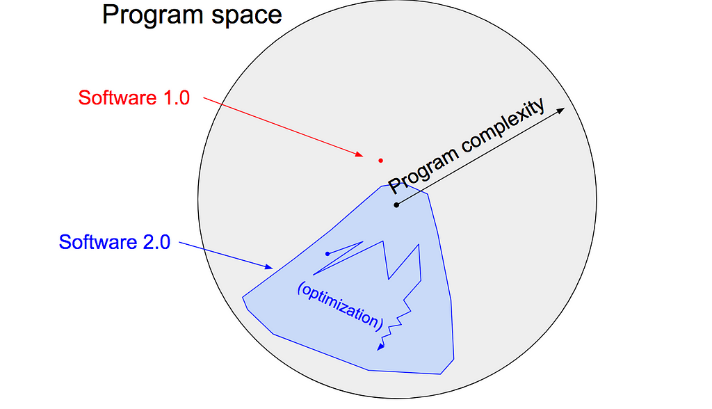
The “classical stack” of Software 1.0 is what we’re all familiar with — it is written in languages such as Python, C++, etc. It consists of explicit instructions to the computer written by a programmer. By writing each line of code, the programmer identifies a specific point in program space with some desirable behavior.

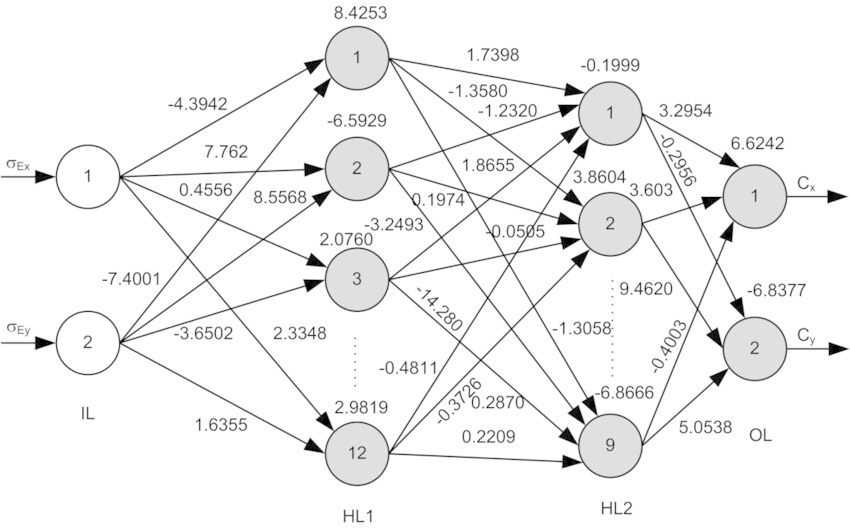
In contrast, Software 2.0 can be written in much more abstract, human unfriendly language, such as the weights of a neural network. No human is involved in writing this code because there are a lot of weights (typical networks might have millions), and coding directly in weights is kind of hard (I tried).

Instead, our approach is to specify some goal on the behavior of a desirable program (e.g., “satisfy a dataset of input output pairs of examples”, or “win a game of Go”), write a rough skeleton of the code (e.g. a neural net architecture), that identifies a subset of program space to search, and use the computational resources at our disposal to search this space for a program that works. In the specific case of neural networks, we restrict the search to a continuous subset of the program space where the search process can be made (somewhat surprisingly) efficient with backpropagation and stochastic gradient descent.

It turns out that a large portion of real-world problems have the property that it is significantly easier to collect the data (or more generally, identify a desirable behavior) than to explicitly write the program. In these cases, the programmers will split into two teams. The 2.0 programmers manually curate, maintain, massage, clean and label datasets; each labeled example literally programs the final system because the dataset gets compiled into Software 2.0 code via the optimization. Meanwhile, the 1.0 programmers maintain the surrounding tools, analytics, visualizations, labeling interfaces, infrastructure, and the training code.

Ongoing transition

Let’s briefly examine some concrete examples of this ongoing transition. In each of these areas we’ve seen improvements over the last few years when we give up on trying to address a complex problem by writing explicit code and instead transition the code into the 2.0 stack.

Visual Recognition used to consist of engineered features with a bit of machine learning sprinkled on top at the end (e.g., an SVM). Since then, we discovered much more powerful visual features by obtaining large datasets (e.g. ImageNet) and searching in the space of Convolutional Neural Network architectures. More recently, we don’t even trust ourselves to hand-code the architectures and we’ve begun searching over those as well.

Speech recognition used to involve a lot of preprocessing, gaussian mixture models and hidden markov models, but today consist almost entirely of neural net stuff. A very related, often cited humorous quote attributed to Fred Jelinek from 1985 reads “Every time I fire a linguist, the performance of our speech recognition system goes up”.

Speech synthesis has historically been approached with various stitching mechanisms, but today the state of the art models are large ConvNets (e.g. WaveNet) that produce raw audio signal outputs.

Machine Translation has usually been approaches with phrase-based statistical techniques, but neural networks are quickly becoming dominant. My favorite architectures are trained in the multilingual setting, where a single model translates from any source language to any target language, and in weakly supervised (or entirely unsupervised) settings.

Games. Explicitly hand-coded Go playing programs have been developed for a long while, but AlphaGo Zero (a ConvNet that looks at the raw state of the board and plays a move) has now become by far the strongest player of the game. I expect we’re going to see very similar results in other areas, e.g. DOTA 2, or StarCraft.

Databases. More traditional systems outside of Artificial Intelligence are also seeing early hints of a transition. For instance, “The Case for Learned Index Structures” replaces core components of a data management system with a neural network, outperforming cache-optimized B-Trees by up to 70% in speed while saving an order-of-magnitude in memory.

You’ll notice that many of my links above involve work done at Google. This is because Google is currently at the forefront of re-writing large chunks of itself into Software 2.0 code. “One model to rule them all” provides an early sketch of what this might look like, where the statistical strength of the individual domains is amalgamated into one consistent understanding of the world.

The benefits of Software 2.0

Why should we prefer to port complex programs into Software 2.0? Clearly, one easy answer is that they work better in practice. However, there are a lot of other convenient reasons to prefer this stack. Let’s take a look at some of the benefits of Software 2.0 (think: a ConvNet) compared to Software 1.0 (think: a production-level C++ code base). Software 2.0 is:

Computationally homogeneous. A typical neural network is, to the first order, made up of a sandwich of only two operations: matrix multiplication and thresholding at zero (ReLU). Compare that with the instruction set of classical software, which is significantly more heterogenous and complex. Because you only have to provide Software 1.0 implementation for a small number of the core computational primitives (e.g. matrix multiply), it is much easier to make various correctness/performance guarantees.

Simple to bake into silicon. As a corollary, since the instruction set of a neural network is relatively small, it is significantly easier to implement these networks much closer to silicon, e.g. with custom ASICs, neuromorphic chips, and so on. The world will change when low-powered intelligence becomes pervasive around us. E.g., small, inexpensive chips could come with a pretrained ConvNet, a speech recognizer, and a WaveNet speech synthesis network all integrated in a small protobrain that you can attach to stuff.

Constant running time. Every iteration of a typical neural net forward pass takes exactly the same amount of FLOPS. There is zero variability based on the different execution paths your code could take through some sprawling C++ code base. Of course, you could have dynamic compute graphs but the execution flow is normally still significantly constrained. This way we are also almost guaranteed to never find ourselves in unintended infinite loops.

Constant memory use. Related to the above, there is no dynamically allocated memory anywhere so there is also little possibility of swapping to disk, or memory leaks that you have to hunt down in your code.

It is highly portable. A sequence of matrix multiplies is significantly easier to run on arbitrary computational configurations compared to classical binaries or scripts.

It is very agile. If you had a C++ code and someone wanted you to make it twice as fast (at cost of performance if needed), it would be highly non-trivial to tune the system for the new spec. However, in Software 2.0 we can take our network, remove half of the channels, retrain, and there — it runs exactly at twice the speed and works a bit worse. It’s magic. Conversely, if you happen to get more data/compute, you can immediately make your program work better just by adding more channels and retraining.

Modules can meld into an optimal whole. Our software is often decomposed into modules that communicate through public functions, APIs, or endpoints. However, if two Software 2.0 modules that were originally trained separately interact, we can easily backpropagate through the whole. Think about how amazing it could be if your web browser could automatically re-design the low-level system instructions 10 stacks down to achieve a higher efficiency in loading web pages. With 2.0, this is the default behavior.

It is better than you. Finally, and most importantly, a neural network is a better piece of code than anything you or I can come up with in a large fraction of valuable verticals, which currently at the very least involve anything to do with images/video and sound/speech.

The limitations of Software 2.0

The 2.0 stack also has some of its own disadvantages. At the end of the optimization we’re left with large networks that work well, but it’s very hard to tell how. Across many applications areas, we’ll be left with a choice of using a 90% accurate model we understand, or 99% accurate model we don’t.

The 2.0 stack can fail in unintuitive and embarrassing ways ,or worse, they can “silently fail”, e.g., by silently adopting biases in their training data, which are very difficult to properly analyze and examine when their sizes are easily in the millions in most cases.

Finally, we’re still discovering some of the peculiar properties of this stack. For instance, the existence of adversarial examples and attacks highlights the unintuitive nature of this stack.

Programming in the 2.0 stack

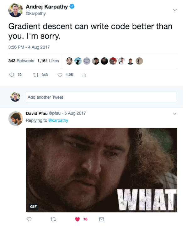
Software 1.0 is code we write. Software 2.0 is code written by the optimization based on an evaluation criterion (such as “classify this training data correctly”). It is likely that any setting where the program is not obvious but one can repeatedly evaluate the performance of it (e.g. — did you classify some images correctly? do you win games of Go?) will be subject to this transition, because the optimization can find much better code than what a human can write.

The lens through which we view trends matters. If you recognize Software 2.0 as a new and emerging programming paradigm instead of simply treating neural networks as a pretty good classifier in the class of machine learning techniques, the extrapolations become more obvious, and it’s clear that there is much more work to do.

In particular, we’ve built up a vast amount of tooling that assists humans in writing 1.0 code, such as powerful IDEs with features like syntax highlighting, debuggers, profilers, go to def, git integration, etc. In the 2.0 stack, the programming is done by accumulating, massaging and cleaning datasets. For example, when the network fails in some hard or rare cases, we do not fix those predictions by writing code, but by including more labeled examples of those cases. Who is going to develop the first Software 2.0 IDEs, which help with all of the workflows in accumulating, visualizing, cleaning, labeling, and sourcing datasets? Perhaps the IDE bubbles up images that the network suspects are mislabeled based on the per-example loss, or assists in labeling by seeding labels with predictions, or suggests useful examples to label based on the uncertainty of the network’s predictions.

Similarly, Github is a very successful home for Software 1.0 code. Is there space for a Software 2.0 Github? In this case repositories are datasets and commits are made up of additions and edits of the labels.

In the short/medium term, Software 2.0 will become increasingly prevalent in any domain where repeated evaluation is possible and cheap, and where the algorithm itself is difficult to design explicitly. And in the long run, the future of this paradigm is bright because it is increasingly clear to many that when we develop AGI, it will certainly be written in Software 2.0.

cool! 🙂

there’s something subtle also going on in the objective with the entropy regularization, which is inserted into policy gradients to incetivise exploration.

The side of effect of this is that the optimal agent behavior will actually be to act randomly when it doesn’t matter. In Pong, the final agent therefore jitters around randomly with maximum entropy, but when it comes to catching the ball, executing the precise sequence of moves needed to get that done. And then reverting back to random behavior.