It’s now possible to associate GitHub, AWS CodeCommit, and any self-hosted Git repository with Amazon SageMaker notebook instances to easily and securely collaborate and ensure version-control with Jupyter Notebooks. In this blog post, I’ll elaborate on the benefits of using Git-based version-control systems and how to set up your notebook instances to work with Git repositories.

Data science projects demand collaborative effort. Data scientists, machine learning developers, data engineers, analysts, and business decision-makers need to share insights, delegate tasks, and review the history of their work to ensure a healthy journey from ideation to productization of machine learning models. Git-based version-control systems allow us to centralize data science practices in a sharable environment. By using Git repositories with Jupyter Notebooks, we can coauthor projects, track code changes, and amalgamate software engineering and data science practices for production-ready code management.

Additionally, notebooks in a notebook instance are stored on durable Amazon Elastic Block Store (EBS) volumes. However, they don’t persist beyond the life of the notebook instance. That means that if you delete your notebook instance, you will lose your work. Storing notebooks in a Git repository enables you to decouple Jupyter Notebooks from the instance lifecycle and keep them as standalone documents that can be referenced and reused in the future.

Finally, most of the publicly available content about machine learning and deep learning techniques are provided on Jupyter Notebooks that are hosted in Git repositories, such as GitHub. Cloning these notebooks seamlessly onto your notebook instances speeds up the learning process by allowing you to easily discover, execute, and share the publicly available learning material.

There are two ways to associate Git repositories with Amazon SageMaker notebook instances:

• If you want to clone a public Git repository, which doesn’t require any credentials, you can simply provide the URL for the repository while creating a notebook instance. Amazon SageMaker will kick off your instance with the Git repository cloned onto it.
• If you want to associate a private Git repository that requires credentials or personal access token, or if you want to store public Git repository information for future use, you first need to add this Git repository as a resource in your Amazon SageMaker account. When you add a Git repository that requires authentication, you can specify an AWS Secrets Manager secret that contains credentials or personal access token to access the repository. After you add a Git repository as a resource, you can create and use as many notebook instances as you need to be associated with this repository.

Since it’s comprehensive, I’ll walk you through the second use case where we introduce a private Git repository to Amazon SageMaker as a resource and create a notebook instance that is associated with this Git repository.

Add a Git repository to your Amazon SageMaker account

You can add Git repositories to your Amazon SageMaker account in the AWS Management Console or by using the AWS CLI.

To add a Git repository to Amazon SageMaker using the AWS Management Console, open the Amazon SageMaker console at https://console.aws.amazon.com/sagemaker/.

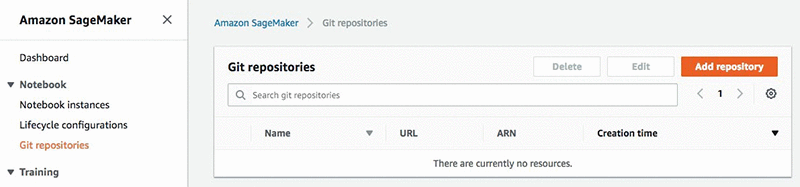
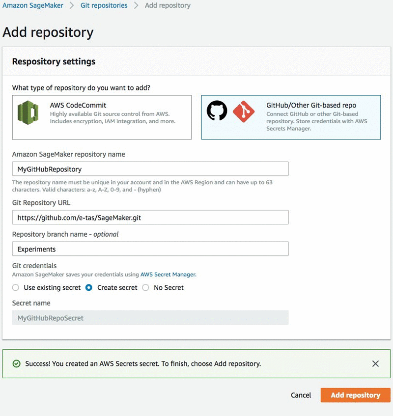
In the left navigation pane, choose Git repositories, which provides a centralized visibility and management for all of your Git repositories. Choose Add repository.

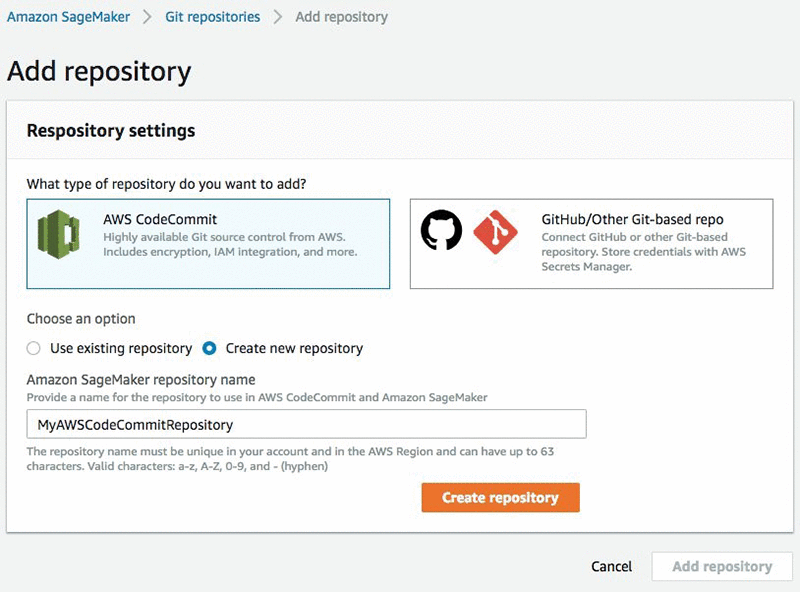
To add an AWS CodeCommit repository, choose AWS CodeCommit. Here, you can create a new AWS CodeCommit repository or use an existing one. Please note that the repository name must be 1 to 63 characters. Valid characters are a-z, A-Z, 0-9, and – (hyphen).

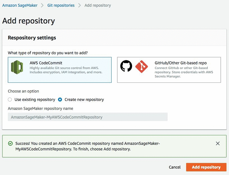
If you are creating a new AWS CodeCommit repository, the action button to Add repository will be active after your AWS CodeCommit repository is created.

To add a Git repository hosted somewhere other than AWS CodeCommit, choose GitHub/Other Git-based repo.

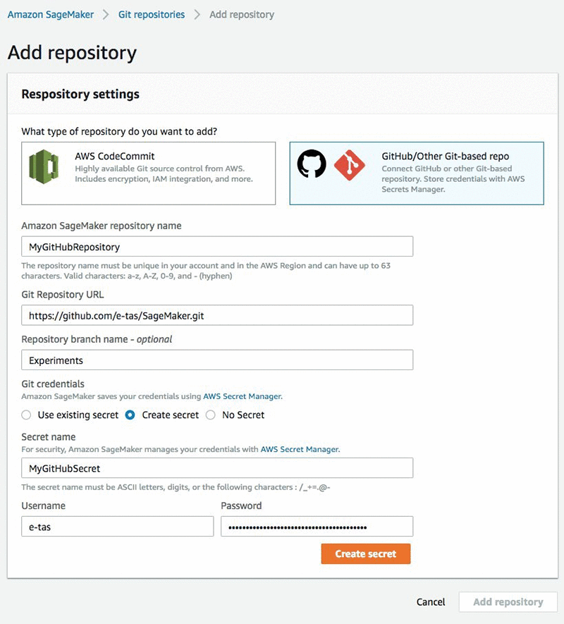
Enter the URL for the repository and a name to use for the repository in Amazon SageMaker. The name must be 1 to 63 characters. Valid characters are a-z, A-Z, 0-9, and – (hyphen).

For Git credentials, enter the credentials to use to authenticate to the repository. For GitHub repositories, instead of your account password, we strongly recommend using a Personal Access Token generated by your Git service provider due to its convenience and safety.

Amazon SageMaker uses AWS Secrets Manager behind the scenes to securely store Git credentials for private Git repositories that require authentication. Here, you can either create a new AWS Secrets Manager secret or choose an existing one. For more information about AWS Secrets Manager secrets or about using your company’s LDAP credentials with AWS Secrets Manager, see the AWS Secrets Manager User Guide.

If you are creating a new secret to store your credentials, the action button to Add repository will be active after your new secret is created.

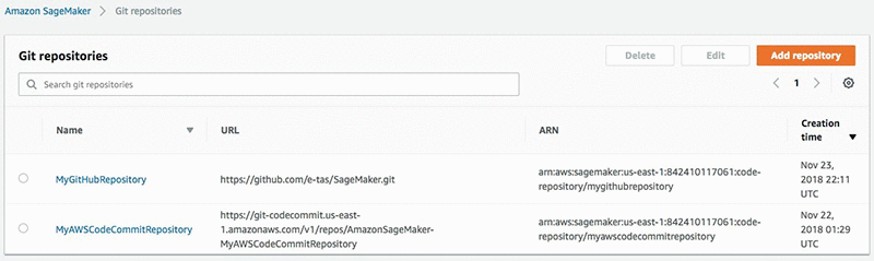
You can view and manage all Git repositories that you have associated with Amazon SageMaker under the Git repositories menu.

To add a Git repository to Amazon SageMaker using the CLI, use the create-code-repository AWS CLI command.

If you are adding a private Git repository other than AWS CodeCommit, you first need to create an AWS Secrets Manager secret to store your credentials and obtain the Amazon Resource Name (ARN) of the AWS Secrets Manager secret to provide while using create-code-repository AWS CLI command.

Ensure that your IAM role has a policy update to give you permission to access for GetSecretValue.

Also, the secret must be in the following format:

{“username”: UserName, “password”: Password}

If you are adding a public Git repository, you don’t need an AWS Secrets Manager secret.

Specify a name for the repository as the value of the code-repository-name argument. The name must be 1 to 63 characters. Valid characters are a-z, A-Z, 0-9, and – (hyphen). Specify the default branch, the URL of the Git repository, and the Amazon Resource Name (ARN) of an AWS Secrets Manager secret that contains the credentials to use to authenticate the repository as the value of the git-config argument.

The following command creates a new repository named MyRespository in your Amazon SageMaker account that points to a Git repository hosted at https://github.com/myprofile/my-repo”.

aws sagemaker create-code-repository  --code-repository-name "MyRepository"  --git-config '{"Branch":"master",  "RepositoryUrl" : "https://github.com/myprofile/my-repo",  "SecretArn" : "arn:aws:secretsmanager:us-east-2:012345678901:secret:my-secret-ABc0DE"}'

Create a notebook instance with associated Git repositories

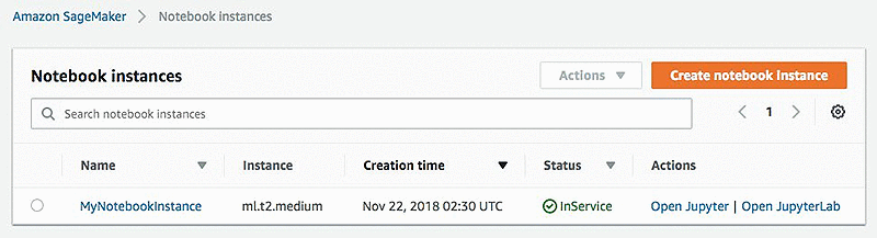
To create an instance with Git repositories cloned to it, go to Notebook instances on the Amazon SageMaker console, and choose Create notebook instance.

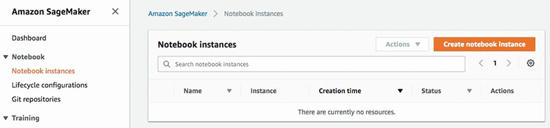
Follow the steps described in the Amazon SageMaker Developer Guide for other configurations, such as Amazon Virtual Private Cloud (VPC) or AWS Identity and Access Management (IAM).

You can  use existing AWS CodeCommit repositories that you have not created with Amazon SageMaker, but directly with AWS CodeCommit. However, you need to ensure that you have either added the “AmazonSageMaker-” prefix to the name of the repository (for example, AmazonSageMaker-MyAWSCodeCommitRepository) or that you have updated the IAM policy for your notebook instance’s execution role to grant permission to Amazon SageMaker for accessing your AWS CodeCommit repository. Update the IAM policy for your notebook instance’s execution role to have codecommit:GitPull and codecommit:GitPush permissions. For a full list of AWS CodeCommit permissions, see the AWS CodeCommit User Guide.

To clone Git repositories, use the menu to specify which repositories you want to clone:

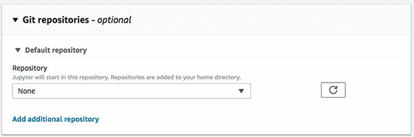
Here, if you want to use a public repository that you haven’t added or don’t want to add to your Amazon SageMaker account, you can select Clone a public Git repository to this notebook instance only. In this case, you can simply paste the public URL for the repository, and Amazon SageMaker will clone it to your notebook instance.

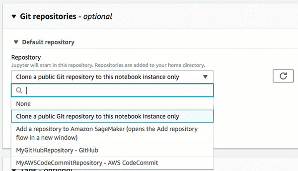
You can also select Add a repository to Amazon SageMaker, which will lead you to the previous menu where we added repositories to Amazon SageMaker.

Finally, you can see the repositories that you have added to Amazon SageMaker on the menu. If you just added a repository and don’t see it yet on the menu, try to refresh the menu by using the refresh button.

You can select one default repository and up to three additional repositories to be associated with your notebook instance.

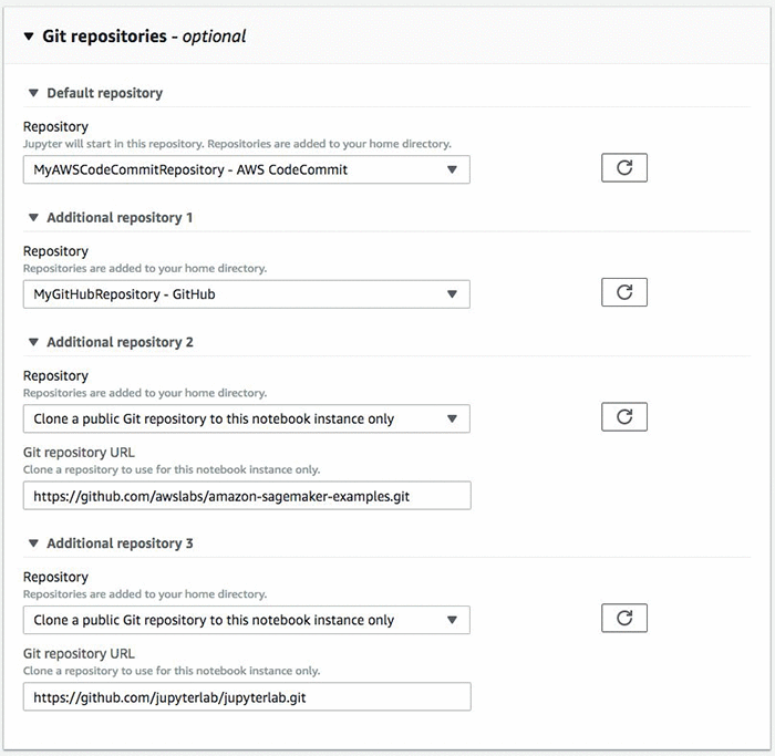
Your notebook instance will be created with the Git repositories cloned to it.

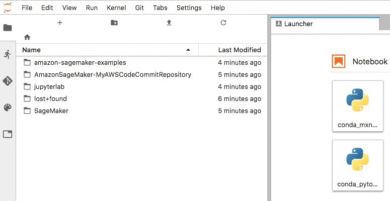
Open JupyterLab to see your repositories on the left menu.

If you prefer to execute these actions using CLI commands, refer to the Amazon SageMaker Developer Guide for the details.

Using Git repositories in a notebook instance

Your notebook instance will open in the default repository, which is installed in your notebook instance under /home/ec2-user/SageMaker. You can manually run Git commands in a notebook cell. For example:

!git pull origin master

To open any of the additional repositories, navigate up one folder. The additional repositories are also installed as directories under /home/ec2-user/SageMaker.

In collaboration with the Project Jupyter community, the Amazon SageMaker team has redesigned and developed an open-source Git extension for JupyterLab. If you are not a fan of CLI commands, the Git extension provides an intuitive and visual way to collaborate on JupyterLab. You can use the Git extension to create and switch branches, stage and commit code changes, send push and pull requests to shared repositories, see the version history in detail, and revert to previous versions when needed.

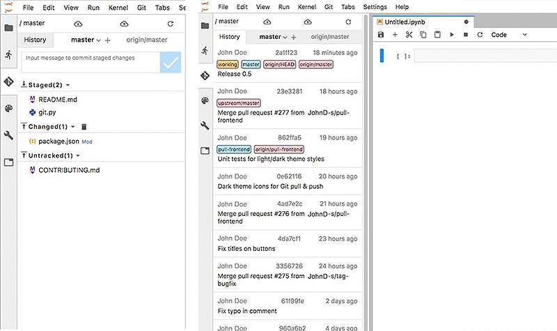
If you open the notebook instance with a JupyterLab interface, the jupyter-git extension is installed and available to use. For information about the JupyterLab Git extension, visit the JupyterLab GitHub page.

Conclusion

By using Git workflows easily with notebooks, you will be able to clone content to your JupyterLab workbench, participate in multiple-coauthor projects, and branch your data science work within the organization’s broader development and production workflows.

About the Author

Erkan Tas is a Senior Product Manager for Amazon SageMaker. He is on a mission to make Artificial Intelligence easy, accessible, and scalable through AWS platforms. He is also a sailor, science and nature admirer, Go and Stratocaster player.

Amazon SageMaker is a managed and infinitely scalable machine learning (ML) platform. With this platform, it is easy to build, train, and deploy machine learning models. Amazon SageMaker already has two popular built-in computer vision algorithms for image classification and object detection. The Amazon SageMaker image classification algorithm learns to categorize images into a set of pre-defined categories. The Amazon SageMaker object detection algorithm learns to draw bounding boxes and identify objects in the boxes. Today, we are excited to announce that we are enhancing our computer vision family of algorithms with the launch of the Amazon SageMaker semantic segmentation algorithm.

An example of the Amazon SageMaker semantic segmentation algorithm at work. Photo by Pixabay via PEXELS.

Semantic segmentation (SS) is the task of classifying every pixel in an image with a class from a known set of labels. The segmentation output is usually represented as different RGB (or grayscale, if the number of classes is fewer than 255) values. Therefore the output is a matrix (or grayscale image)  with the same shape as the input image. This output image is also called a segmentation mask. With the Amazon SageMaker semantic segmentation algorithm, you can train your models with your own dataset, plus you can use our pre-trained models for favorable initialization. The algorithm is built using the MXNet Gluon framework and the Gluon CV toolkit. It provides an option of three built-in, state-of-the-art algorithms with which you can learn the semantic segmentation model:

• The fully-convolutional network (FCN)
• The pyramid-scene-parsing network (PSP)
• The DeepLab-V3

All algorithms have two distinct components:

• An encoder or a backbone
• A decoder.

The backbone is a network that produces reliable activation maps of image features. The decoder is a network that constructs the segmentation mask from the encoded activation maps. Amazon SageMaker semantic segmentation provides a choice of pre-trained or randomly initialized ResNet50 or ResNet101 as options for backbones. The backbones come with pre-trained artifacts that were originally trained on the ImageNet classification task. These are reliable pre-trained artifacts that users can use to fine-tune their FCN or PSP backbones for segmentation. Alternatively, users can initialize these networks from scratch. Decoders are never pre-trained.

The algorithm can be trained using P2/P3 type  Amazon Elastic Compute Cloud (Amazon EC2) instances in single machine configurations. Trained models from the algorithm can be hosted on all CPU and GPU instances supported by Amazon SageMaker. However, training on CPU machines is always more expensive than GPU machines since we are able to make use of advanced math libraries to fully use GPUs for convolutional networks. Therefore, we restrict training only to GPU machines. When trained and properly hosted, the algorithm can either generate segmentation masks for a query image as a PNG file or produce a probability score for each pixel for each class. The algorithm can handle a variety of segments of varying sizes, shapes and scales natively.

Getting started

Amazon SageMaker semantic segmentation expects the customer’s training dataset to be on Amazon Simple Storage Service (Amazon S3). Once trained, it produces the resulting model artifacts on Amazon S3. Amazon SageMaker takes care of starting and stopping Amazon EC2 instances for the customers during training. After the model is trained, it can be deployed to an endpoint. For a general, high-level overview of the Amazon SageMaker workflow, see the Amazon SageMaker documentation. The Amazon SageMaker semantic segmentation algorithm can be trained using several interfaces. The AWS Management Console interface has a simple form-like structure that can be used to kick off training jobs and creating endpoints. There are also APIs that are available in Python that are explained using the associated notebook.

I/O format

The Amazon SageMaker semantic segmentation algorithm will supports the following file input format. This format allows the user to directly pass images. The dataset in Amazon S3 is expected to be presented in four channels: two for train and two for validation using four directories, two for images and two for annotations. Annotations are expected to be uncompressed PNG images. The dataset may also have a label map that describes how the annotation mappings are established. If not, a default will be used. The algorithm is capable of working with annotations from various annotation systems and standard benchmarking datasets. The algorithm also supports an augmented manifest for PIPE mode training straight from S3. Refer to the documentation on how the I/O format works. The algorithm allows inputs to be supplied using an augmented manifest, which works in Pipe mode straight from S3.

Inference formats

To query a trained model using the model’s endpoint, an image needs to be supplied along with an Accept Type denoting the type of output required. Depending on the request, the algorithm will output a PNG file with a segmentation mask in the same format as the labels itself, or it outputs class probabilities encoded in a protobuf format. Refer to the documentation for more information on AcceptTypes.

Training job

Note that the Amazon SageMaker semantic segmentation algorithm only supports GPU instances for training. We recommend using GPU instances with more memory for training with large batch sizes.  While the algorithm trains, you can monitor the progress through either at the Amazon SageMaker notebook or Amazon CloudWatch. After the training is done, the trained model artifacts will be uploaded to the Amazon S3 output location that you specified in the training configuration. To deploy the model as an endpoint, you can choose to use either a CPU or a GPU instance.

Performance numbers

The following numbers demonstrate some performance numbers for the Amazon SageMaker semantic segmentation algorithm. We trained on the PASCAL VOC12  training dataset and observe the mean Intersection-over-Union (mIOU) on the VOC12  validation dataset with a crop size of  240X240.  For the experiment, we used backbone = "resnet-50" and “rmsprop” as the optimizer with default parameters (momentum = 0.9, weight_decay = 0.0001). We trained the model for 20 epochs and achieved an mIOU of 0.62. Using backbone="resnet-50", we observe an approximately 5.83x speedup in training speed while going from a single GPU (ml.p3.2xlarge) to 8 GPUs in (ml.p3.16xlarge) instances with a mini_batch_size of 8 for the former and 64 for the latter. Analogously, we also observed greater than 2.5x speed increase when moving from ml.p2.16xlarge to ml.p3.16xlarge multi-GPU instances.

Notebooks

An example of object detection is available in the SageMaker notebooks repository. Refer to this for a complete tutorial and some recommendations for data preparation and hyperparameters.

Conclusion

In this blog post we announced the launch of the Amazon SageMaker Semantic Segmentation algorithm. We described how to get started with training your own semantic segmentation models, and we presented a few performance numbers. We look forward to hearing from you as you set up your own implementation of semantic segmentation.

About the Authors

Ragav Venkatesan is a Research Scientist with AWS AI Labs. He has an MS in Electrical Engineering and a PhD in Computer Science from Arizona State University. His current area of research includes Neural Network compression and Computer Vision algorithms for Amazon SageMaker. Outside of work, Ragav is a session bassist and producer at Thaalam Studios.

Saksham Saini did his BS in Computer Engineering from University of Illinois at Urbana-Champaign. He is currently working on building highly optimized and scalable algorithms for Amazon SageMaker. Outside work, he enjoys reading, music and traveling.

Satyaki Chakraborty is an MS student at Carnegie Mellon University studying computer vision. He contributed to Amazon SageMaker Semantic Segmentation during his summer internship.

Xiong Zhou is an Applied Scientist with AWS AI Labs. He has a PhD in Electrical and Electronics Engineering from University of Houston. His current research focus involves developing domain adaptation and active learning algorithms. He is also working on building computer vision algorithms for Amazon SageMaker.

Luka Krajcar is a Software Development Engineer on the AWS AI Algorithms team. He received his M.S. in Computer Science at the Faculty of Electrical Engineering and Computing at the University of Zagreb. Outside of work, Luka enjoys reading fiction, running, and video gaming.

Hang Zhang is an Applied Scientist with Amazon AI. He has a PhD from Rutgers University. He is currently working with the GluonCV team.

Amazon Translate is a neural machine translation service that delivers fast, high-quality, and affordable language translation. Today, we are introducing Custom Terminology, a feature that customers can use to customize Amazon Translate output to use company- and domain-specific vocabulary. By uploading and invoking Custom Terminology with translation requests, customers have the ability to ensure that their unique content, such as brand names, character names, and model names, is translated exactly the way they need it, regardless of context and the Amazon Translate algorithm’s decision.

To Illustrate, consider the following example. “Amazon Family” is a collection of benefits that offers Amazon Prime members exclusive offers, such as up to 20% off subscriptions to diapers, baby food, and more. This is very useful if you have a couple of diaper-wearers at home like I do. In France, we call it “Amazon Famille.” If I try to translate “Amazon Family” into French using Amazon Translate without any additional context, I get the output “Famille Amazon.” This is an accurate translation, but it is not what the team in France needs. Now, if I try adding context, for example “Have you ever shopped with Amazon Family?”, the service determines that the program name does not need to be translated, and leaves it as is: “Avez-vous déjà fait des achats avec Amazon Family?”. This is a good translation too but still not what our team is looking for. To solve for this and similar problems, we are introducing the Custom Terminology feature. By adding an entry that says that the term “Amazon Family” should be translated as “Amazon Famille” to their Custom Terminology, the team can make sure that “Amazon Family” is translated into “Amazon Famille,” regardless of context. “Amazon Family” will now be translated into “Amazon Famille” and “Have you ever shopped with Amazon Family?” will now be translated into “Avez-vous déjà fait des achats avec Amazon Famille?”

Why is this important?

All of our customers want accurate and fluent translations regardless of where and how they use Amazon Translate. But some customers tell us that when they use the service to translate company-authored content like product documentation, website strings, functional content, knowledge bases, and help pages, they have another requirement. They need translations to adhere to the company’s specific vocabulary, and in some cases to the industry or domain jargon. In tests we ran, we saw that customizing output with Custom Terminology more than doubled the amount of times the service gets specific terminology right. To our customers, this means more accurate translations that translate (no pun intended) into better engagement with applications built with Amazon Translate powering multilingual content. This means fewer translations that need to be edited by professional translators, thus cutting costs and time to market.

How does it work?

Generally speaking, the engine works as follows: When a translation request comes in, Amazon Translate reads the source sentence, creates a semantic representation of the content (simply put — “understands it”), and generates a translation into the target language word after word.

When a Custom Terminology is invoked as part of the translation request, the engine scans the terminology file before returning the final result. When it identifies an exact match between a terminology entry and a string in the source text, it locates the appropriate string in the proposed translation and replaces it with the terminology entry. In the Amazon Family example, it first generates the translation “Avez-vous déjà fait des achats avec Amazon Family?” but stops and replaces “Amazon Family” with “Amazon Famille”, before providing the response.

When should I use Custom Terminology?

First, note that Amazon Translate is trained on billions of parallel words, from a wide range of domains. As in the Amazon Family example, in many cases, Amazon Translate can distinguish named entities and handle them as required “out of the box”. Second, understand that, at this point, the Custom Terminology feature is an override mechanism. It does NOT train a custom model based on your organization’s terminology. It finds a match and replaces it. It does not transform content in any way, nor does it behave differently depending on the context. For example, in the Amazon Family case, if I had references to the Amazon Family brand and also to the Amazon family of employees (and for some reason the word Family was capitalized in the latter) within the same body of text, applying the terminology would have degraded the translation quality. Therefore, while we do not limit the acceptable types of input, we strongly recommend that users follow the following best practices. Any deviation from them is likely to result in translation quality degradation.

Best practices

1. Do keep your terminology minimal. Only include completely unambiguous words that you want to control/preserve. These should be words that you want to be translated in only one way. Ideally, you should limit the list to proper names, like brand names and product names.
2. For every term, do include any transformations of the source phrase you want to control for separately. E.g., for plural and possessive in that language (e.g., Amazon, Amazon’s) or capitalization (e.g., AMAZON, amazon).
3. Do NOT include different translations for the same source phrase (e.g., entry #1 — EN: Amazon, FR: Amazon, entry #2 – EN: Amazon FR: Amazone).
4. Some languages do not change the shape of a word based on sentence context. Applying Custom Terminology per these guidelines is most likely to improve overall translation quality. Other languages have extensive word shape changes. We do NOT recommend applying the feature to those languages, but do not restrict you from doing so. The following list of languages can help guide you:
   

   Languages	Compatibility
   East Asian Languages (e.g., Chinese, Japanese, Korean, Indonesian)	Compatible
   Germanic Languages (German, Dutch, English, Swedish, Danish)	Compatible
   Romance Languages (Italian, French, Spanish, Portuguese)	Compatible
   Hebrew	Compatible
   Slavic Languages (Russian, Polish, Czech)	Incompatible
   Finno-Ugric Languages (Finnish)	Incompatible
   Arabic	Incompatible
   Turkish	Incompatible

How do I use it?

Get started with Custom Terminology by reviewing the documentation pages here to understand best practices and the formatting requirements to ensure your files are readable. Then create and upload your terminology using the console or supported SDKs. Once your terminology file is accepted, you can make translation requests to the service coupled with Custom Terminology. When matches are found, the translation results will automatically replace applicable content with terminology entries. For more details, visit the documentation page.

To get started with Amazon Translate go to Getting Started with Amazon Translate or check out this 10 minute video tutorial.

About the Author

Yoni Friedman is a Sr. Technical Product Manager in the AWS Artificial Intelligence team where he leads product management for Amazon Translate. He spends his free time reading, running, playing ball, and doing other stuff his two toddlers ask him to.

We are excited to announce Amazon Comprehend Medical, a new HIPAA-eligible machine learning service that allows developers to process unstructured medical text and identify information such as patient diagnosis, treatments, dosages, symptoms and signs, and more. Comprehend Medical helps health care providers, insurers, researchers, and clinical trial investigators as well as health care IT, biotech, and pharmaceutical companies to improve clinical decision support, streamline revenue cycle and clinical trials management, and better address data privacy and protected health information (PHI) requirements.

The majority of health and patient data is stored today as unstructured medical text, such as medical notes, prescriptions, audio interview transcripts, and pathology and radiology reports. Identifying this information today is a manual and time consuming process, which either requires data entry by high skilled medical experts, or teams of developers writing custom code and rules to try and extract the information automatically. In both cases this undifferentiated heavy lifting takes material resources away from efforts to improve patient outcomes through technology.

Improving medical language processing with machine learning

Amazon Comprehend Medical allows developers to identify the key common types of medical information automatically, with high accuracy, and without the need for large numbers of custom rules. Comprehend Medical can identify medical conditions, anatomic terms, medications, details of medical tests, treatments and procedures. Ultimately, this richness of information may be able to one day help consumers with managing their own health, including medication management, proactively scheduling care visits, or empowering them to make informed decisions about their health and eligibility.

There are no servers to provision or manage – developers only need to provide unstructured medical text to Comprehend Medical. The service will “read” the text and then identify and return the medical information contained within it. Comprehend medical will also highlight protected health information (PHI). There are no models to train and no ML experience is required. And, no data processed by the service is stored or used for training. Through the Comprehend Medical API, these new capabilities can be integrated with existing services and health systems easily. The service is also covered under AWS’s HIPAA eligibility and BAA.

Unlocking this information from medical language makes a variety of common medical use cases easier and cost-effective, including: clinical decision support (e.g., getting a historical snapshot of a patient’s medical history), revenue cycle management (e.g., simplifying the time-intensive manual process of data entry), clinical trial management (e.g., by identifying and recruiting patients with certain attributes into clinical trials), building population health platforms, and helping address (PHI) requirements (e.g., for privacy and security assurance.)

From Hours To Seconds In Cancer Care

We are working closely with Seattle’s own Fred Hutchinson Cancer Research Center – known as Fred Hutch to Seattleites – to support their goals to eradicate cancer in the future. Comprehend Medical is helping to identify patients for clinical trials who may benefit from specific cancer therapies. Fred Hutch was able to evaluate millions of clinical notes to extract and index medical conditions, medications, and choice of cancer therapeutic options, reducing the time to process each document from hours, to seconds.

“Curing cancer is, inherently, an issue of time,” said Matthew Trunnell, Chief Information Officer, Fred Hutchinson Cancer Research Center. “For cancer patients and the researchers dedicated to curing them, time is the limiting resource. The process of developing clinical trials and connecting them with the right patients requires research teams to sift through and label mountains of unstructured medical record data. Amazon Comprehend Medical will reduce this time burden from hours per record to seconds. This is a vital step toward getting researchers rapid access to the information they need when they need it so they can find actionable insights to advance lifesaving therapies for patients.”

Another customer AWS who has been previewing the service is Roche Diagnostics.

“Roche’s NAVIFY decision support portfolio provides solutions that accelerate research and enable personalized healthcare. With petabytes of unstructured data being generated in hospital systems every day, our goal is to take this information and convert it into useful insights that can be efficiently accessed and understood,” said Anish Kejariwal, Director of Software Engineering for Roche Diagnostics Information Solutions. “Amazon Comprehend Medical provides the functionality to help us with quickly extracting and structuring information from medical documents, so that we can build a comprehensive, longitudinal view of patients, and enable both decision support and population analytics.”

Improving patient care through technology is a passion we share with our health care IT and ecosystem customers. We’re extremely excited about the role that Comprehend Medical can play in supporting that mission.

Today we are excited to announce the availability of Dynamic Training (DT) for deep learning models, or DT for short. DT allows deep learning practitioners to reduce model training cost and time by leveraging the cloud’s elasticity and economies of scale. Our first reference implementation of DT is based on Apache MXNet, and is open sourced under Dynamic Training with Apache MXNet. This blog post introduces the concept of DT, showcases training results achieved, and demonstrates how you can get started leveraging it for your model training jobs.

Distributed Training of deep learning models

Training neural networks is a repetitive process in which the network is fed with batches of training data, the loss and the gradient are calculated, and model parameters are updated iteratively until a sufficient accuracy is achieved. For state-of-the-art deep learning models, the process becomes extremely computationally intensive as both the number of model parameters and the number of training samples becomes extremely large. For example, ResNet-50 [1], a modern image classification model, contains around 25 million parameters, and the IMAGENET labeled dataset, often used to train models such as ResNet-50, contains more than 14 million images, while industry datasets are often 10 times larger. Indeed, training a network such as ResNet-50 with the IMAGENET dataset on a single host can take days. To reduce the training time of deep networks, practitioners typically use distributed training, which distributes the training job across multiple hosts, thus reducing the overall training time. Distributed multi-host training is supported in modern deep learning frameworks such as Apache MXNet and TensorFlow. It can be used to reduce training time significantly: The team at Sony recently demonstrated training ResNet50 on IMAGENET in 224 seconds using 2176 Nvidia Tesla V100 GPUs.

Introducing Dynamic Training

Traditional distributed training requires a fixed number of hosts that are actively participating in the training job throughout the training process. With DT, this requirement is relaxed: the number of hosts in the training cluster is allowed to fluctuate, growing and shrinking throughout the training process. This relaxed property of DT enables training jobs to leverage key advantages of the cloud: compute elasticity and cost reduction. The AWS Cloud provides rapid access to flexible and low-cost IT resources such as compute, and allows customers to benefit from the cloud’s massive economies of scale through products such as Amazon Elastic Compute Cloud (EC2) Spot Instances. Spot Instances offer spare compute capacity in the AWS Cloud at steep discounts, up to 90 percent, compared to standard On-Demand Instances.

With DT, practitioners running compute-intensive training jobs can benefit from these economies of scale, and reduce training costs by pulling in Spot Instances when available, and releasing them when they are interrupted, all without stopping the training job. DT allows practitioners to cut down on model training cost significantly, as well as reduce training time by increasing the training cluster size when possible.

In addition, DT enables practitioners to better utilize their organization’s pool of Amazon EC2 Reserved Instances. Practitioners can pull Reserved Instances into the training job when available, and release instances back to the Reserved Instances pool when instances are required for other, more critical applications, all while allowing the training job to continue without interruption. The following diagram shows the DT process using the Reserved Instances pool.

Dynamic Training of ResNet-50 with Apache MXNet

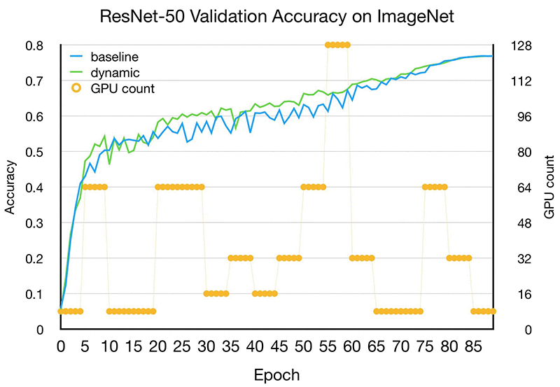
Now let’s go over some results. With our implementation of Dynamic Training with Apache MXNet, we were able to train ResNet-50 v1 [1], a deep convolutional model for image classification, on the IMAGENET dataset, without loss of accuracy. The elastic training job used a pool of P3.16xlarge instances, each consisting of 8 Tesla V100 GPUs. Throughout the 90 epochs training process, the number of hosts in the training cluster fluctuated up and down between 8 GPUs and 96 GPUs.

Because the number of hosts may be changed across training epochs, DT fixes the total batch size, while dynamically adjusting the mini-batch size per GPU based on the number of hosts participating in the given epoch. The following chart illustrates how the DT process utilized a dynamic training cluster, and how it performed compared to the baseline fixed cluster training. Note that both training sessions converged on the same target validation accuracy by the 90th epoch.

This example, alongside other experiments that we ran, demonstrated that DT reduces cost to train by 15 to 50 percent, and reduces time to train by 15 to 30 percent. The actual time and cost reductions vary because they depend on the model architecture, the training cluster setup, and the type of instances used.

“We are running computer vision models developed in MXNet to measure the freshness of waffle fries. To reduce the training time of neural networks, we wanted to use distributed training,” said Jay Duff, Management Consultant, Chick-Fil-A. “Dynamic Training with Apache MXNet on AWS allows us to better utilize the AWS infrastructure by elastically adding EC2 Spot and Reserved Instances to training jobs. We expect to reduce training costs by up to 20 percent.”

Getting started with Dynamic Training

To get started with DT with Apache MXNet, visit the GitHub repository, and follow the example. Currently, the implementation supports only Apache MXNet and EC2 Reserved Instances.  We plan to add support for Spot Instances, as well as additional deep learning frameworks, in the future.

We’d love to hear your feedback and experience using DT to train your models. Your feedback on issues and your contributions on the GitHub repository are welcomed!

[1] He, Kaiming, et al. “Deep residual learning for image recognition.” Proceedings of the IEEE conference on computer vision and pattern recognition. 2016.

About the authors

Vikas Kumar – Vikas is Senior Software Engineer for AWS Deep Learning, focusing on building scalable deep learning systems. Prior to this Vikas has worked on building service discovery systems for microservices and databases. In his spare time he enjoys reading and music.

Haibin Lin – Haibin is a Software Development Engineer for AWS Deep Learning, focusing on distributed optimization and natural language processing. In his spare, he enjoys hiking and traveling.

Andrea Olgiati – Andrea is a Principal Engineer for AWS Deep Learning, focusing on building scalable machine learning systems. Prior to this, he worked on databases, compilers, and microchips. In his spare time he enjoys playing the piano and lifting heavy things.

Mu Li – Mu Li is a principal scientist for machine learning at AWS. Before joining AWS, he was the CTO of Marianas Labs, an AI start-up. He also served as a principal research architect at the Institute of Deep Learning at Baidu. He obtained his PhD in computer science from Carnegie Mellon University. He enjoys spending time with his family.

Hagay Lupesko – Hagay is an Engineering Leader for AWS Deep Learning. He focuses on building deep learning systems that enable developers and scientists to build intelligent applications. In his spare time, he enjoys reading, hiking, and spending time with his family.

Today, I’m excited to share that, for the first time, the same machine learning courses used to train engineers at Amazon are now available to all developers through AWS.

We’ve been using machine learning across Amazon for more than 20 years. With thousands of engineers focused on machine learning across the company, there are very few Amazon retail pages, products, fulfillment technologies, stores which haven’t been improved through the use of machine learning in one way or another. Many AWS customers share this enthusiasm, and our mission has been to take machine learning from something which had previously been only available to the largest, most well-funded technology companies, and put it in the hands of every developer. Thanks to services such as Amazon SageMaker, Amazon Rekognition, Amazon Comprehend, Amazon Transcribe, Amazon Polly, Amazon Translate, and Amazon Lex, tens of thousands of developers are already on their way to building more intelligent applications through machine learning.

Regardless of where they are in their machine learning journey, one question I hear frequently from customers is: “how can we accelerate the growth of machine learning skills in our teams?” These courses, available as part of a new AWS Training and Certification Machine Learning offering, are now part of my answer.

There are more than 30 self-service, self-paced digital courses with more than 45 hours of courses, videos, and labs for four key groups: developers, data scientists, data platform engineers, and business professionals. Each course starts with the fundamentals, and builds on those through real-world examples and labs, allowing developers to explore machine learning through some fun problems we have had to solve at Amazon. These include predicting gift wrapping eligibility, optimizing delivery routes, or predicting entertainment award nominations using data from IMDb (an Amazon subsidiary). Coursework helps consolidate best practices, and demonstrates how to get started on a range of AWS machine learning services, including Amazon SageMaker, AWS DeepLens, Amazon Rekognition, Amazon Lex, Amazon Polly, and Amazon Comprehend.

New AWS Certification for Machine Learning

To help developers demonstrate their knowledge (and to help employers hire more efficiently), we are also announcing the new “AWS Certified Machine Learning – Specialty” certification. Customers can take the exam now (and at half price for a limited time). Customers at re:Invent can sit for the exam this week at our Training and Certification exam sessions.

The digital courses are now available at no charge at aws.training/machinelearning and you only pay for the services you use in labs and exams during your training.

–Dr. Matt Wood, General Manager of Artificial Intelligence, AWS

Today we are announcing updates to our face detection, analysis, and recognition features. These updates provide customers with improvements in the ability to detect more faces from images, perform higher accuracy face matches, and obtain improved age, gender, and emotion attributes for faces in images. Amazon Rekognition customers can use each of these enhancements starting today, at no additional cost. No machine learning experience is required.

“Face detection” tries to answer the question: Is there a face in this picture? In real-world images, various aspects can have an impact on a system’s ability to detect faces with high accuracy. These aspects might include pose variations caused by head movement and/or camera movements, occlusion due to foreground or background objects (such as faces covered by hats, hair, or hands of another person in the foreground), illumination variations (such as low contrast and shadows), bright lighting that leads to washed out faces, low quality and resolution that leads to noisy and blurry faces, and distortion from cameras and lenses themselves. These issues manifest as missed detections (a face not detected) or false detections (an image region detected as a face even when there is no face). For example, on social media different poses, camera filters, lighting, and occlusions (such as a photo bomb) are common. For financial services customers, verification of customer identity as a part of multi-factor authentication and fraud prevention workflows involves matching a high resolution selfie (a face image) with a lower resolution, small, and often blurry image of face on a photo identity document (such as a passport or driving license). Also, many customers have to detect and recognize faces of low contrast from images where the camera is pointing at a bright light.

With the latest updates, Amazon Rekognition can now detect 40 percent more faces – that would have been previously missed – in images that have some of the most challenging conditions described earlier. At the same time, the rate of false detections is reduced by 50 percent. This means that customers such as social media apps can get consistent and reliable detections (fewer misses, fewer false detections) with higher confidence, allowing them to deliver better customer experiences in use cases like automated profile photo review. In addition, face recognition now returns 30 percent more correct ‘best’ matches (the most similar face) compared to our previous model when searching against a large collection of faces. This enables customers to obtain better search results in applications like fraud prevention. Face matches now also have more consistent similarity scores across varying lighting, pose, and appearance, allowing customers to use higher confidence thresholds, avoid false matches, and reduce human review in applications such as identity verification. As always, for use cases involving civil liberties or customer sentiments, where the veracity of the match is critical, we recommend that customers use best practices, higher confidence level (at least 99%), and always include human review.

Now let’s look at some images to see how Amazon Rekognition handles the various aspects of challenging images captured in unconstrained environments.

Pose variations

This issue is encountered in faces captured from acute camera angles (like shots taken from above or below a face), shots with side-on view of a face, or when the subject is looking away. This issue is typically seen in social media photos (for example, when a subject is looking into the distance), selfies, or fashion photoshoots. Face detection algorithms have difficulty in detecting such faces because less than half the face might be visible in many cases, or the faces might be tilted at uncommon angles (like being upside down).

Image 1: Side-on view of faces

Image 2: Faces looking down at the camera at various angles

Image 3: Person looking into the sky and away from the camera

Difficult lighting

Lighting might be challenging due to low contrast, low light setups, or extreme contrast. This pattern is common in stock photography and at event venues. Face detection algorithms can struggle with such examples because there is either not enough contrast between face features and the background in low lighting, or, alternatively, face features can be washed out due to bright lighting, again making them difficult to discern.

Image 4: Bright lighting on face

Image 5: Low contrast and shadows on a face

Image 6: Extreme contrast

Blur or occlusion

This challenge is seen in photos that have artistic effects (selfies or fashion photos, video motion blur), partial occlusion by objects, paint or hair (fashion photography), or less-than ideal sharpness (photos taken from identity documents). All of the features of the face are not clearly visible clearly in such cases, so face detection is challenging.

Image 7: Face obstructed by hair

Image 8: Face obstructed by hands and other objects

Face detection and recognition updates are now available in all AWS Regions supported by Amazon Rekognition except AWS GovCloud  – US East (N. Virginia), US East (Ohio), US West (Oregon), EU West (Ireland), Asia Pacific (Tokyo), Asia Pacific (Mumbai), Asia Pacific (Seoul), and Asia Pacific (Sydney). To get started, you can try the latest version in the Amazon Rekognition console and refer to the documentation.

About the Authors

Ranju Das has been with Amazon for almost five years and leads Amazon Rekognition, a deep learning-based image recognition service which allows you to search, verify and organize millions of images. Before joining Amazon, Ranju worked at Barnes and Noble leading Nook Cloud engineering. His team was responsible for strategy, design, development and SaaS operation of Nook mobile services and Digital Asset Management Services.

Venkatesh Bagaria is a Senior Product Manager for Amazon Rekognition. He focuses on building powerful but easy-to-use deep learning-based image and video analysis services for AWS customers. In his spare time, you’ll find him watching way too many stand-up comedy specials and movies, cooking spicy Indian food, and trying to pretend that he can play the guitar.

Conversational interfaces are transforming the way people interact with software applications and services. They are untethering people from keyboards and smartphone gestures by replacing those interfaces with a more natural style of interaction: the spoken word. Increasingly, people are opting to interact with a bot when they need an answer to a question, to set a reminder, or to obtain a product or service.

With Amazon Lex, we can bring this same level of convenience to data. By allowing users to explore datasets by asking a series of questions, and maintaining a conversational context, we can provide a whole new experience and relationship with data.

This blog post shows you how to use Amazon Lex to implement a business intelligence (BI) chatbot, which we refer to as “BIBot,” although you can customize it to use a different name. BIBot can respond to user questions about data in a database, by converting the questions into backend database queries, and transforming the result sets into natural language responses. For example, the request “tell me the increase in inventory last month” could be translated to “select sum(item_qty) from inventory where month(received_date) = 10”.

BIBot has been integrated with a typical relational database intended for business intelligence and reporting applications. The sample database is the Amazon Redshift TICKIT database, which tracks sales activity for a fictional website where users buy and sell tickets online for music concerts and theater shows. The database is a star schema with two fact tables (sales, listings) and five dimension tables (events, dates, venues, categories, and users). See Amazon Redshift » Sample Database for details.

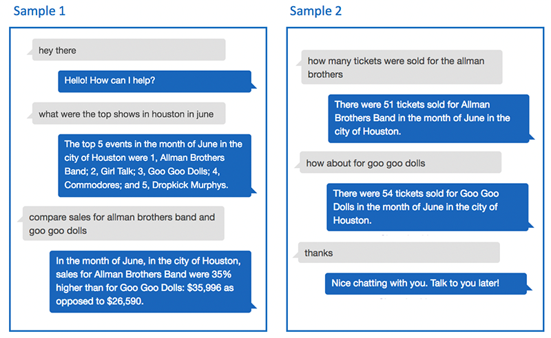
Here are some sample interactions with BIBot:

As you can see from these examples, BIBot is able to keep track of the context of your questions, by remembering that you asked about Houston in June, and that you asked how many tickets were sold. The conversation uses the “language” of the data, which in this case is ticket sales, cities, months, events, and so on. These are the facts and dimensions of the sample ticket sales database. If you adapt BIBot to use your reporting database, conversations with the bot will be in the language of your data.

Architecture

BIBot’s architecture is simple. A Lex bot directs each of the user’s questions to an intent, which parses the question into slots. The Amazon Lex bot then passes the intent and slot data to an AWS Lambda function, which uses the data to construct a SQL query, and execute it against an Amazon Athena database. Athena retrieves the query results from a set of CSV files stored in an Amazon S3 bucket, and returns the result set back to the Lambda function, which converts it into a natural language response.

Athena was used for simplicity and convenience, but this architecture will work with any SQL-based database, and can be adapted to other types of data sources, such as NoSQL databases.

Installing BIBot

To get started, let’s install the sample Amazon Lex bot in your AWS account. To make it easy to install BIBot, and for you to make subsequent changes, we’ve implemented a pipeline using AWS CodePipeline that uses AWS CodeBuild to create and update the Amazon Lex bot, the Lambda intent handler functions, and the Athena database.

Step 1: Fork the public amazon-lex-bi-bot into your own GitHub account.

By creating your own copy of the BIBot codebase, you can experiment by making changes to the bot, and even modify it to use your data. Any time you commit a change to your repo, the pipeline will rebuild your bot for you.

Note: if you don’t already have a GitHub account, you can create one for free at https://github.com.

Step 2: Store your AWS API credentials in AWS Systems Manager Parameter Store

The CodeBuild project will make AWS API calls to build the Amazon Lex bot, Lambda function, and Athena database. To do this, it will require your AWS API credentials. If you don’t already have the AWS CLI set up in your environment, follow the directions here: Configuring the AWS CLI. In the AWS Management Console, go to the AWS Systems Manager console, and choose Shared Resources, then choose Parameter Store. Create two parameters with the following parameter names and values:

• ACCESS_KEY_ID – paste in the value of your aws_access_key_id from your AWS credentials file
• SECRET_ACCESS_KEY – paste in the value of your aws_secret_access_key from your credentials file

To protect these sensitive keys, make sure to select the Secure String type for each parameter, so that the values are encrypted in Parameter Store.

Step 3: Create the pipeline using AWS CloudFormation

Use this button to launch the AWS CloudFormation stack in the us-east-1 AWS Region (N. Virginia):

Enter bibot for the Stack Name. Enter your GitHub username in the Owner field, and for Personal Access Token you can generate a token with Repo scope on GitHub.

Accept the default values for the other parameters, and choose Next twice to display the Review page. Select the acknowledgement check box, and choose Create.

The CloudFormation template will take a minute or two to finish, and it will create the following resources:

In the AWS Management Console, go to the CodePipeline console and open “bibot-pipeline”. You should see two stages, Source and Build. When both stages have succeeded, your Amazon Lex bot is built.

Next, go to the CodeBuild console and choose Build history. You should see an entry for the “bibot-build” project. Choose the Build run link and inspect the Build details, Environment variables, and Build logs.

Step 4: Copy the sample TICKIT data to your AthenaBucket S3 bucket

When your CloudFormation stack has finished launching, the Output tab will contain AWS CLI commands to copy the data files from the Amazon Redshift sample TICKIT database to your new AthenaBucket S3 bucket. For example:

$ aws s3 cp s3://awssampledbuswest2/tickit/allevents_pipe.txt s3://bibot-athenabucket-xxxxxxxxxxxxx/event/allevents_pipe.txt --source-region us-west-2

Copy each of these AWS CLI commands and execute them to make a copy of the sample data. The Athena database created by CloudFormation uses this data. In the AWS Management Console, go to the Athena console, select the “tickit” database, and try a SQL query. For example:

SELECT DISTINCT event_name from event ORDER BY event_name

Step 5: Test the Lex bot, and refresh its “event_name” slot from the database

Next, got to Amazon Lex, and open BIBot. You will see a warning that you are about to give Amazon Lex permission to invoke your Lambda function, which is expected, so choose OK.

Choose the “event_name” Slot type, and you will see that there are only two entries for this slot (“Sample Event 1” and “Another Sample Event”). Now choose Test Chatbot to open the Lex simulator, and type (or say) “refresh yourself”. BIBot will read the list of events from the database and update the “event_name” Slot type. Choose the “event_name” Slot type again to see the events – you should see a list of event names such as “Joshua Radin,” “Jessica Simpson,” “Nine Inch Nails,” etc.

You will now need to rebuild your bot. Return to the Amazon Lex console, select the BIBot Lex bot, and choose Build. BIBot is now ready for testing – open the Lex simulator and ask BIBot some questions!

Lex bot design

The BIBot Lex bot has eight intents:

The Hello and GoodBye intents are simple, and included mainly just to add character. You can say “Hello,” “hey there,” “hi,” and so on, and BIBot will respond. When you’re done, if you want, you can say “thanks,” “bye,” “good job,” “catch you later,” etc., and BIBot will end the session.

Top, Compare, Count, Switch, and Reset are more interesting. These intents are designed to implement a conversational, natural language interface for specific types of database queries. They’re flexible, because they can work with any of the dimensions in the database, and they’re coordinated, because they remember and share context as the user asks a series of questions as part of a larger conversation.

The Refresh intent updates the definition of a Lex slot type with dimension data from the database (in this case, the list of event names from the EVENT table in the sample TICKIT database).

Let’s take a look at the Top intent:

This intent allows you to ask questions like, “Tell me the top 3 events in Boston,” or “What were the top cities for Dave Matthews Band in March.”

This intent uses the following slots:

• {count} – uses the built-in AMAZON.NUMBER slot type.
• {dimension} – a custom slot type, identifying dimensions from the sample database: “events,” “months,” “venues,” “cities,” “states,” and “categories.” This slot type also uses synonyms, so that you can say “locations” instead of “venues,” for example.

Each of the dimensions in the sample database are also represented as slots:

• {event_name} – a custom slot type, identifying the set of events that exist in the sample TICKIT database “EVENT” table. This slot type is updated via the Refresh
• {event_month} – uses the built-in AMAZON.Month slot type.
• {venue_name} – uses the built-in AMAZON.MusicVenue slot type.
• {venue_city} – uses the built-in AMAZON.US_CITY slot type.
• {venue_state} – uses the built-in AMAZON.US_STATE slot type
• {cat_desc} – a custom slot type, identifying the set of categories that exist in the sample TICKIT database “CATEGORY” table.

Building a domain-specific natural language

BIBot’s query intents – Top, Compare, Count, Switch, and Reset – all work in this way: they use slots as the “vocabulary” needed to build sentence structures relevant to the underlying dataset. In effect, BIBot’s intents implement a domain-specific natural language. The Amazon Lex powerful natural language understanding capabilities make this easy to do.

As an example, take a look at some sample utterances from the Count intent:

When you ask BIBot “How many tickets were sold for the Allman Brothers in Arlington in February?” the Lex natural language processing engine is able to parse the question correctly, by using components from several of the sample utterances. You don’t need to specify every permutation of every question in the sample utterances.

Maintaining conversational context

When you ask BIBot a question, the Lambda fulfillment function responds with an answer, but also retains some of the slot values in session attributes, which are shared across intents. This allows BIBot to carry on a conversation, in effect remembering what was previously asked. Maintaining conversational context in this way is key to providing a more natural user experience, and for simplifying the ability for users to explore a dataset by asking a series of related questions.

For example, in the sample interaction at the beginning of this blog, the user asked about the top shows in Houston in June, and BIBot identified the top five events. When the user asked to compare sales for the Allman Brothers and the Goo Goo Dolls, BIBot “understood” that this was a follow-on question, and that the user really wanted to compare the sales for those events in Houston, in June. This approach enables the user to drill down on their results until they find the information they need.

Sometimes a user may want to back up, switch gears, broaden the search results, or just start over. BIBot’s Top, Compare, and Count query intents support this, with some additional help from the Reset intent. For example:

Sourcing slots from the data

As noted previously, BIBot uses built-in Amazon slot types to represent some of the dimensions, including the month, city, state, and venue name. For the event name dimension, the Refresh intent reads the data from the database and updates the corresponding slot types using the aws.lex-models.put-slot-type API call. This trains the Amazon Lex NLU engine to recognize event names specific to the TICKIT database. For frequently changing datasets, the Refresh intent logic could be triggered automatically on a scheduled basis.

Amazon Lex can correctly identify the intended slots even when they include values that might also exist in other slot types, as shown in the following examples. Lex is able to recognize “Boston” and “Chicago” as bands, as well as cities, even in the same request.

AWS Lambda implementation and extensibility

BIBot’s Python-based Lambda fulfillment functions consist of intent handlers, helper functions, configuration data, and user exit functions. There are eight intent handler functions:

• hello_intent.py
• count_intent.py
• compare_intent.py
• top_intent.py
• switch_intent.py
• reset_intent.py
• refresh_intent.py
• goodbye_intent.py

Helper functions include:

• get_slot_values(slot_values, intent_request)
• remember_slot_values(slot_values, session_attributes)
• get_remembered_slot_values(slot_values, session_attributes)
• execute_athena_query(query_string)
• close(session_attributes, fulfillment_state, message)

All of these functions are database agnostic, and can be configured to work for different database schemas.

Configuration parameters include slot configuration, dimension information, and SQL query strings, which are specific to the underlying database. Slots are configured to match the slot types defined for the intents:

SLOT_CONFIG = {
  'event_name':  {'type': TOP_RESOLUTION, 'remember': True,  
                  'error': 'I did not find an event called "{}".'},
  'event_month': {'type': ORIGINAL_VALUE, 'remember': True},
  'venue_name':  {'type': ORIGINAL_VALUE, 'remember': True},
  'venue_city':  {'type': ORIGINAL_VALUE, 'remember': True},
  'venue_state': {'type': ORIGINAL_VALUE, 'remember': True},
   ...
}

BIBot also needs to understand the dimensions for the database, and how they map to database columns:

DIMENSIONS = {
  'events':     {'slot': 'event_name',  'column': 'e.event_name',  'singular': 'event'},
  'months':     {'slot': 'event_month', 'column': 'd.month',       'singular': 'month'},
  'venues':     {'slot': 'venue_name',  'column': 'v.venue_name',  'singular': 'venue'},
  'cities':     {'slot': 'venue_city',  'column': 'v.venue_city',  'singular': 'city'},
  'states':     {'slot': 'venue_state', 'column': 'v.venue_state', 'singular': 'state'},
  'categories': {'slot': 'cat_desc',    'column': 'c.cat_desc',    'singular': 'category'}
}

The query intent handlers need SQL queries that are specific to the database. For example, here are the configuration parameters for the Top intent handler for the sample TICKIT database:

TOP_SELECT  = "SELECT {}, SUM(s.amount) ticket_sales FROM sales s, event e, venue v, "            
              "category c, date_dim d " 
TOP_JOIN    = " WHERE e.event_id = s.event_id AND v.venue_id = e.venue_id AND "  
              " c.cat_id = e.cat_id AND d.date_id = e.date_id "
TOP_WHERE   = " AND LOWER({}) LIKE LOWER('%{}%') " 
TOP_ORDERBY = " GROUP BY {} ORDER BY ticket_sales desc" 

The “{ }” parameters are replaced by column names and values at runtime based on the user’s request.

In addition to configuration parameters, there are user exit functions:

• pre_process_query_value(key, value)
• post_process_slot_value(key, value)
• post_process_dimension_output(key, value)
• get_state_name(value)
• get_month_name(value)
• post_process_venue_name(venue)

These functions are called prior to inserting values into query parameters or after extracting them from the result set, in order to allow mappings between human-readable values and the values stored in the database. You can insert custom code in these functions to implement database-specific mappings.

For example, when the user asks for the top five events in California, preprocess_query_value() converts the value to “CA” which corresponds to the data in the database. The post_process_dimension_output() performs the reverse function, converting the value “CA” returned from the database to back to “California”.

Conclusion

Natural language interfaces will change the way that people interact with data. Traditional business intelligence dashboards, visualizations, and alerts will be augmented with conversational interfaces, in which business users find answers to their questions about their data simply by asking.

BIBot provides an extensible framework for implementing a conversational interface for business data. It’s designed to be integrated with traditional reporting database structures, such as star schemas or snowflake schemas, but can be adapted to other types of data sources, such as NoSQL databases. The sample implementation includes three simple analytics – top aggregates by dimension, compare aggregates for two dimensions, and count an aggregate – which can all participate together seamlessly within a shared conversational context. Additional analytics can be added to this framework, from simple queries to complex simulations and predictive models.

Give BIBot a try with your business data, and let us know how it works for your organization!

About the Author

Brian Yost is a Senior Consultant with AWS Professional Services. In his spare time, he enjoys mountain biking, home brewing, and tinkering with technology.

We’ve seen a ton of progress in machine learning during the past 12 months, with customers using Amazon SageMaker – a fully-managed service which has put ML into the hands of tens of thousands of developers and data scientists – to find fraud, predict pitches, and tune engines. We’ve added nearly 100 new features and capabilities since we introduced SageMaker at re:Invent last year, with the vast majority based on customer feedback (keep it coming). We continue that drum beat today, with major new announcements for Amazon SageMaker.

Introducing SageMaker Workflows

Today, we’re announcing new automation, orchestration, and collaboration features for Amazon SageMaker to make it easier to build, manage, and share machine learning workflows.

Machine learning is a highly collaborative process – combining domain experience with technical skills is the bedrock of success, and often requires multiple iterations and experimentation with different datasets and features. Developers often need to share progress and gather feedback from many collaborators. Training a successful model is almost never a hole-in-one, and so it’s important to be able to keep track of the important decisions, replay the successful parts, reuse what worked, and get help on what didn’t. We’re introducing new capabilities to make these iterations easier to manage, repeat, and share.

Experiment Management with SageMaker Search

Developing a successful ML model requires continuous experimentation, trying new algorithms and model hyperparameters, all the while observing the impact of potentially small changes on performance and accuracy. This iterative exercise means it can be hard to track which unique combination of datasets, algorithms, and parameters brewed the “winning” model.

Data scientists and developers can now organize, track, and evaluate their machine learning model training experiments with Amazon SageMaker Search. SageMaker Search lets you quickly find and evaluate the most relevant model training runs from the potentially thousands of Amazon SageMaker model training runs, right from the AWS console.

Collaboration with Version Control

Data scientists, developers, data engineers, analysts, and business leaders often need to share ideas, tasks, and collaborate to make progress with machine learning. The de-facto standard for this type of collaboration with traditional software development has been version control. It plays an important role in ML too, and we’re making it easier by adding Git integration and visualization to Amazon SageMaker.

Customers can now link GitHub, AWS CodeCommit, or self-hosted Git repositories with SageMaker notebooks, clone public and private repositories, and store repository information in Amazon SageMaker securely using IAM, LDAP, and AWS Secrets Manager. You can review your branches, merges, and versions directly in SageMaker, using a new open source notebook app.

Automation with Step Functions & Apache Airflow

ML often requires multiple steps in a complete workflow to be run in a coordinated sequence. For example, you may want to perform a query in Amazon Athena or aggregate and prepare data in AWS Glue, before training a model in SageMaker, and deploying it to production. Automating these steps and orchestrating them across multiple services helps build reusable, reproducible ML workflows which can be shared between engineers and scientists.

You can now use Step Functions to automate and orchestrate SageMaker steps in an end-to-end workflow. You can automate publishing datasets to Amazon S3, training an ML model on your data with SageMaker, and deploying your model for prediction. AWS Step Functions will monitor SageMaker (and Glue) jobs until they succeed or fail, and either transition to the next step of the workflow or retry the job. It includes built-in error handling, parameter passing, state management, and a visual console that lets you monitor your ML workflows as they run.

In addition to Step Functions, many developers currently use Apache Airflow, a popular open source framework to author, schedule, and monitor multi-stage workflows. Amazon SageMaker now also integrates with Airflow, so you can use the same orchestration tool you’re used to to drive SageMaker tasks such as data preparation, training, and tuning. If you’re new to Airflow, you can spin up a new instance and start orchestrating workflows on AWS in just a few clicks, using CloudFormation.

These new features will be available to customers to take for a test drive, starting early next month.

New Algorithms and Frameworks

Not that long ago, part of the ‘cost of doing business’ with machine learning was significant investment in research and development of new algorithms; both in achieving the right levels of accuracy, and in bringing those algorithms out of the lab and into the real world where they could run across large, complex training datasets. Customers can run algorithms for training models in three ways in SageMaker; by bringing their own in a custom container, by using built-in SageMaker Algorithms, or by running fully-managed MXNet, TensorFlow, PyTorch, and Chainer algorithms with just 20 lines of code. We’ve been adding new algorithms through the year too, including BlazingText for text classification, and Object Detection in images.

We’re pleased to announce new built-in algorithms for detecting suspicious IP addresses (IP Insights), low dimensional embeddings for high dimensional objects (Object2Vec), and – an oldie but a goodie – unsupervised grouping (K-means clustering), all designed to support petabyte scale datasets, at 10x better performance than you would expect to see with traditional methods. Without needing an entire R&D department, any developer can access these algorithms as they would any other API in SageMaker, and get the benefit of fast, low cost training, even at scale.

We’ve also been adding new framework support through the year (including PyTorch 1.0 and Chainer) and keeping others up to date (such as the latest MXNet 1.3), and we’re pleased to announce that customers will soon also be able to run fully-managed Horovod jobs for high scale distributed training, and scikit-learn and Spark MLeap for inference.

New Compliance Standards and Accreditation

Security, encryption, compliance, and accreditation are all critical areas for machine learning; ensuring you can meet the regulatory and organizational requirements on your data (and data dependent assets such as models and notebooks) is job zero for everyone using ML.

We’re pleased to add SageMaker to our System and Organizational Controls (SOC) Level 1, Level 2, and Level 3 audits. The SOC reports are available now in the AWS Management Console, and you can download the SOC3 report as a PDF. These controls complement SageMaker’s existing accreditations; the service is in scope for ISO 9001:2015, 27001:2013, 27017:2015, 27018:2014, PCI DSS 3.2 Level 1, and is eligible for HIPAA and BAA coverage on AWS. ITAR workloads can be run on SageMaker in the AWS GovCloud (US) region.

Real World Machine Learning with Amazon SageMaker

 These new capabilities, algorithms, and accreditation will help bring more machine learning workloads to more developers. By focusing almost exclusively on what customers are asking for, we’re making real strides in making machine learning useful and usable in the real world through Amazon SageMaker. Accreditation, experimentation, and automation aren’t always the first thing you may think of when it comes to artificial intelligence, but our customers tell us that these features can further shorten the time it takes to build, train, and deploy their models. No R&D department required.

–Dr. Matt Wood, General Manager of Artificial Intelligence, AWS