Today, at the AWS Summit in Santa Clara, California, we kicked off the 2019 season of the world’s first global autonomous racing league. The AWS DeepRacer League allows developers of all skill levels to get hands on with machine learning through a series of live racing events at AWS Global Summits around the world. The AWS DeepRacer League includes virtual events and tournaments throughout the year.

It was an exciting day as developers put their machine learning skills to the test! After 9 hours, 400 autonomously driven laps, and over 5 miles of racing, the Santa Clara winner was declared. Chris Miller, founder of Cloud Brigade, based in Santa Cruz California, topped the leaderboard and will be the first victor to advance on an expenses-paid trip to the AWS DeepRacer Championship Cup at re:Invent 2019 in Las Vegas, Nevada. With a winning time of 10.43 seconds, Chris and his team came to the Santa Clara Summit with the intent to learn more about AI and ML “I’m excited about machine learning and the technology that is being made available for modern applications”. Chris trained his winning model in one of the AWS DeepRacer workshops at the summit. Next on the agenda for Chris –  he is now preparing for re:Invent by learning more about machine learning and how he can customize his model further.

The top three developers on the leaderboard: Chris Miller (Center) Santa Clara Summit Champion, Rahul Shah (left) First Runner Up, Adrian Sarno (Right) Second Runner Up

Machine Learning available for all

The league is only just beginning and you don’t have to be at an AWS Summit to start learning about machine learning with AWS DeepRacer. Today we are launching a new online digital training course called AWS DeepRacer: Driven by Reinforcement Learning. The course is available at no cost as part of AWS Training and Certification, within the AWS Machine Learning Developer Learning Path. The course has 6 self-guided chapters and in 90 minutes will help you prepare to compete in the AWS DeepRacer League. You will learn how to build a reinforcement learning model and find tips and tricks about how to tune those models to climb the leaderboard.

Up next!

The journey to crown the 2019 AWS DeepRacer Champion continues on April 2^nd at the AWS Summit in Paris. Follow the live results on the AWS DeepRacer League webpage. While you’re there, plan your next race. And don’t forget, this competition is open to all. If you don’t have an AWS DeepRacer car or your own model, our Summit pit crew is there to help you select a pre-trained model and race it straight-away. Also, if you can’t make it to any of the in-person events, our virtual circuit is coming soon and will allow anyone, anywhere to compete.

See you on the tracks!

About the Author

Alexandra Bush is a Senior Product Marketing Manager for AWS AI. She is passionate about how technology impacts the world around us and enjoys being able to help make it accessible to all. Out of the office she loves to run, travel and stay active in the outdoors with family and friends.

You’ve collected your datasets, designed your deep neural network architecture, and coded your training routines. You are now ready to run training on a large dataset for multiple epochs on a powerful GPU instance. You learn that the Amazon EC2 P3 instances with NVIDIA Tesla V100 GPUs are ideal for compute-intensive deep learning training jobs, but you have a tight budget and want to lower your cost-to-train.

Spot-instance pricing makes high-performance GPUs much more affordable for deep learning researchers and developers who run training jobs that span several hours or days. Spot instances allow you to access spare Amazon EC2 compute capacity at a steep discount compared to on-demand rates. For an up-to-date list of prices by instance and Region, visit the Spot Instance Advisor. To learn more about the key differences between spot instances and on-demand instances, I recommend going through this Amazon EC2 user-guide.

Spot instances are great for deep learning workflows, but there are a few challenges associated using spot instances versus on-demand instances. First, spot instances can be preempted and can be terminated with just 2 minutes notice. This means you can’t count on your instance to run a training job to completion. Therefore, it’s not recommended for time-sensitive workloads. Second, instance termination can cause data loss if the training progress is not saved properly. Third, if you decide your application should not be interrupted after launching the spot instance, your only option is to stop the spot instance and re-launch as an on-demand or reserved instance.

To address these challenges, here is a step-by-step tutorial on how to set up spot instances for deep learning training workflows while minimizing training progress loss if a spot interruption occurs. My goal is to implement a setup with the following characteristics:

• Decouple compute, storage and code artifacts, and keep the compute instance stateless. This enables easy recovery and training state restore when an instance is terminated and replaced
• Use a dedicated volume for datasets, training progress (checkpoints) and logs. This volume should be persistent and not be affected by instance termination
• Use a version control system (e.g. Git) for training code. This repo should be cloned to commence/resume training. this enables traceability and prevents loss of code changes when instance is terminated
• Minimize code changes to the training script. This ensures that the training script can be developed independently and backup and snapshot operations are performed outside of the training code
• Automate, automate, automate. Automate replacement instance creation after termination, attaching of dataset and checkpoints EBS volume at launch, moving volumes across Availability Zones, performing instance state restore, resuming training, and terminating instance once training is finished

Deep learning with Spot Instances using TensorFlow and the AWS Deep Learning AMI

In this example, I use spot instances and the AWS Deep Learning AMI to train a ResNet50 model on the CIFAR10 dataset. I use TensorFlow 1.12 configured with CUDA 9 available on the AWS Deep Learning AMI version 21. AWS Deep Learning AMIs are updated frequently, check the AWS Marketplace first to make sure you’re using the latest version compatible with your training code. For TensorFlow 1.13 and CUDA 10 use this AWS Deep Learning AMI instead.

I show you how to set up a spot fleet request for deep learning training jobs, which and you use as a starting point for your specific dataset and models.

To follow along, I assume you’ve met the following pre-requisites:

1. You have an AWS account, and AWS CLI tool installed on your host
2. You are familiar with Python and at least one deep learning framework

As you go through the implementation details, you learn everything else required. All the code, configuration files and AWS CLI commands are available on GitHub.

I use the following AWS and open-source services and concepts. Figure 1 shows how all of these fit together in our example.

• AWS CLI: I use the CLI to interact with AWS services. Everything you can do with the CLI can also be done through the AWS console. The CLI will let you automate, which is one of my goals for this example.
• Amazon EC2 spot instance and spot instance requests: Spot requests ensure that the specified number of spot instances are running. Spot fleet places spot requests to meet the target capacity and automatically replenish any interrupted instances.
• AWS Deep Learning AMI: An Amazon machine image with pre-installed deep learning frameworks. In this example, I use the GPU-accelerated TensorFlow framework for training
• Amazon Elastic Block Storage (EBS): A persistent volume to store datasets, checkpoints and logs, that can be attached to a currently running instance
• Amazon EBS snapshots: Snapshots let you back up data on your Amazon EBS volumes to Amazon S3. A snapshot contains all of the information needed to restore your data to a new EBS volume and can be used to migrate volumes to a new Availability Zone.
• Amazon EC2 user data and instance metadata: At instance launch, user data shell script can be executed to perform actions such as attaching volumes, initiating training and clean up. Instance metadata allows an instance to query information about itself such as instance-id for use with use data shell scripts
• Amazon IAM role and policy: Grants EC2 instance permissions to use AWS services on your behalf. Essential to automate everything.

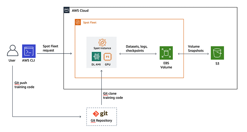
Figure 1: Reference architecture for using spot instances in deep learning workflows

Step 1: Set up a dedicated EBS volume for datasets and checkpoints using a general-purpose instance

The first step is to set up our dedicated EBS volume for storing datasets, checkpoints and other information that needs to persist such as logs and other metadata. This step is only done once so I start by launching an on-demand m4.xlarge instance. If your dataset is small and you’re not going to be performing any pre-processing steps during preparation, then you could launch an instance with lesser memory and processing power that may cost less. If you’re going to be transcoding images or running other multi-threaded pre-processing routines then pick a GPU-backed or compute-optimized CPU instance.

Run the following command on your terminal using the AWS CLI. All the commands listed here were tested on a MacOS.

aws ec2 run-instances 
    --image-id ami-0027dfad6168539c7 
    --security-group-ids <SECURITY_GROUP_ID> 
    --count 1 
    --instance-type m4.xlarge 
    --key-name <KEYPAIR_NAME> 
    --subnet-id <SUBNET_ID> 
    --query "Instances[0].InstanceId"

image-id refers to the Deep Learning AMI Ubuntu instance. Be sure to update the security group, key ID and subnet ID to allow SSH connections into the instance. See this documentation page for more details.

Important: Create a subnet in a specific Availability Zone and remember your choice. EBS volumes can only be attached to instances in the same subnet. See Figure 1 for illustration. In this example I use us-west-2b as my Availability Zone for setup. In step 3 I show you how to automate migration of EBS volumes between Availability Zones using EBS snapshots.

Throughout this example, everything in italics needs to be replaced with values specific to your setup, the rest can just be copied.

Next, create an EBS volume for your datasets and checkpoints. Here I request 100 GiB. You should choose a value that suits your dataset needs. The EBS volume should be in the same Availability Zone as your instance. After you create the volume, attach it to your instance. Specify the ID details from the output of the run-instances and create-volume commands.

aws ec2 create-volume 
    --size 100 
    --region <AWS_REGION> 
    --availability-zone <INSTANCE_AZ> 
    --volume-type gp2 
    --tag-specifications 'ResourceType=volume,Tags=[{Key=Name,Value=DL-datasets-checkpoints}]' 

aws ec2 attach-volume 
    --volume-id vol-<your_volume_id> 
    --instance-id i-<your_instance_id> 
    --device /dev/sdf

Follow the steps in the documentation to connect by using SSH into your instance and then format and mount the attached volume. In this example, I use a mount point directory at root named /dltraining

Do this step only once. Later in step 3 you can see how each new spot instance will automatically self-mount the volume at launch so the datasets and checkpoints are available for training.

In this example I use the following paths:

• Datasets: /dltraining/datasets
• Training progress checkpoints: /dltraining/checkpoints

sudo mkdir /dltraining
sudo mkfs -t xfs /dev/xvdf
sudo mount /dev/xvdf /dltraining
sudo chown -R ubuntu: /dltraining/
cd /dltraining
mkdir datasets
mkdir checkpoints
#
# Optional: Run commands to move your custom datasets into the Datasets directory.
#

To follow along with this example, you can create and then leave these directories empty. The training script ec2_spot_keras_training.py will download the CIFAR10 dataset using Keras, the first-time training is initiated.

You can terminate this instance using the command below. Volume setup is now complete and will persist in the Availability Zone it was created in.

aws ec2 terminate-instances 
    --instance-ids i-<your_instance_id> 
    --output text

Step 2: Create IAM role and policy to grant instance permissions

If you’re new to the cloud, AWS Identity and Access Management (IAM) concepts may be new to you. IAM roles and policies are used to grant instances specific permissions that allow access other AWS services on your behalf.

During training, I want the spot instance to have access to my datasets and checkpoints in the EBS volume I created in step 1. However, only volumes in the same Availability Zone as the instances can be attached to it. If the volume and the instance are in different Availability Zones, a new volume needs to be created using a snapshot of the volume stored in Amazon S3.

All these steps can be performed at instance launch using the AWS CLI and user data bash script, and you can see how in step 3. Here are all the AWS CLI commands you need to run at instance launch:

• Query for volumes with the name tag: DL-datasets-checkpoints (there should be only one)
• Create a snapshot of this volume with tag: DL-datasets-checkpoints-snapshot
• If the instance and volume are in the same Availability Zone, attach volume to the instance
• If the instance and volume are in different Availability Zones, create a new volume from the snapshot in the instance’s Availability Zone with name: DL-datasets-checkpoints, and attach it to the instance. Delete the volume in the different Availability Zone to ensure there is only one copy.
• Once training is complete, cancel the spot fleet request and terminate all training instances

In order for the instance to be able to perform these actions, I will need to grant the instance the permissions to do so on my behalf. This way I don’t grant the instance all the same permissions that I as a user have and risk potential abuse.

I start by first creating a role for my Amazon EC2 instance, called the IAM role. After that I grant specific permissions to this role by creating what is called a policy.  Execute the following command to create a new IAM role. I’ve named my role DL-Training feel free to choose another name.

aws iam create-role 
    --role-name DL-Training 
    --assume-role-policy-document '{"Version":"2012-10-17","Statement":[{"Sid":"","Effect":"Allow","Principal":{"Service":"ec2.amazonaws.com"},"Action":"sts:AssumeRole"}]}'

Next, I will create and attach a policy that grants the instance the following permissions:

1. Describe, create, attach and delete volumes
2. Create snapshots from volumes
3. Describe spot instances
4. Cancel spot fleet requests and terminate instances

You can grant permissions to access other AWS services if you’re going to be using them in your application. In general, the more specific you are about the actions the instance takes the better. The permissions are in a file called ec2-permissions-dl-training.json on the example GitHub repository.

{
    "Version": "2012-10-17",
    "Statement": [
        {
            "Effect": "Allow",
            "Action": [
                "ec2:AttachVolume",
                "ec2:DeleteVolume",
                "ec2:DescribeVolumeStatus",
                "ec2:CancelSpotFleetRequests",
                "ec2:CreateTags",
                "ec2:DescribeVolumes",
                "ec2:CreateSnapshot",
                "ec2:DescribeSpotInstanceRequests",
                "ec2:DescribeSnapshots",
                "ec2:CreateVolume"
            ],
            "Resource": "*"
        }
    ]
}

And run the following to create a policy and attach it to our IAM role:

aws iam create-policy 
    --policy-name ec2-permissions-dl-training  
    --policy-document file://ec2-permissions-dl-training.json
 
aws iam attach-role-policy 
    --policy-arn arn:aws:iam::<account_id>:policy/ec2-permissions-dl-training 
    --role-name DL-Training

Be sure to substitute <account_id> with your AWS account ID in the attach-role-policy command.

Step 3: Create EC2 user data bash script

Next, I create a launch specification file with details about the instance you want to run your training on. In this example I’m going to be using a p3.2xlarge. If you’re running a multi-GPU training job then you can request for an instance with more GPUs. Note, by multi-GPU jobs, I’m referring to multiple GPUs on the same instance. Currently, the maximum number of GPUs you can get on a single instance are 8 GPUs with a p3.16xlarge or p3dn.24xlarge. I cover distributed/multi-node training use-cases in a future blog post.

As discussed in step 2, Amazon EC2 allows you to pass user data shell scripts to an instance that gets executed at launch. Let’s take a look at our user data shell script. The full script (user_data_script.sh) is available on GitHub.

There are 4 key sections in the file:

 Get instance ID and query volume

In this section the script queries the instance metadata API to access to the ID instance on which this script is running. It then uses this information to search for the datasets and checkpoints volume with the tag: DL-datasets-checkpoints

#!/bin/bash

# Get instance ID 
INSTANCE_ID=$(curl -s http://169.254.169.254/latest/meta-data/instance-id)
INSTANCE_AZ=$(curl -s http://169.254.169.254/latest/meta-data/placement/availability-zone)
AWS_REGION=us-west-2

# Get Volume Id and availability zone
VOLUME_ID=$(aws ec2 describe-volumes --region $AWS_REGION --filter "Name=tag:Name,Values=DL-datasets-checkpoints" --query "Volumes[].VolumeId" --output text)
VOLUME_AZ=$(aws ec2 describe-volumes --region $AWS_REGION --filter "Name=tag:Name,Values=DL-datasets-checkpoints" --query "Volumes[].AvailabilityZone" --output text)

Check if the volume and instance are in the same availability zone

In this section the script checks with the volume and the instance are in the same Availability Zone. If they are in different Availability Zones, it first creates a point-in-time snapshot of the volume in Amazon S3. Once the snapshot is created, it deletes the volume and creates a new volume from the snapshot in the instance’s Availability Zone. Figure 2 illustrates the two patterns.

The aws ec2 wait command ensures that snapshot and volume creation are complete before proceeding to the next command.

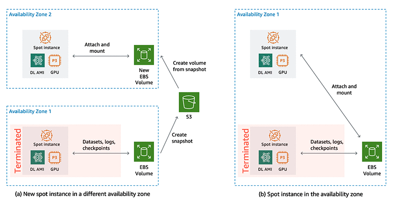
Figure 2: On spot instance termination, if a new spot instance is launched in a different availability zone (a), EBS volume snapshots are saved to S3 and a new volume is created from the snapshot in the instance’s availability zone. If the new spot instance is launched in the same availability zone as the volume (b), the same EBS volume is attached to the new instance

if [ $VOLUME_AZ != $INSTANCE_AZ ]; then
		SNAPSHOT_ID=$(aws ec2 create-snapshot 
				--region $AWS_REGION 
				--volume-id $VOLUME_ID 
				--description "`date +"%D %T"`" 
				--tag-specifications 'ResourceType=snapshot,Tags=[{Key=Name,Value=DL-datasets-checkpoints-snapshot}]' 
				--query SnapshotId --output text)
		aws ec2 wait --region $AWS_REGION snapshot-completed --snapshot-ids $SNAPSHOT_ID
		aws ec2 --region $AWS_REGION  delete-volume --volume-id $VOLUME_ID
		VOLUME_ID=$(aws ec2 create-volume 
				--region $AWS_REGION 
				--availability-zone $INSTANCE_AZ 
				--snapshot-id $SNAPSHOT_ID 
				--volume-type gp2 
				--tag-specifications 'ResourceType=volume,Tags=[{Key=Name,Value=DL-datasets-checkpoints}]' 
				--query VolumeId --output text)
		aws ec2 wait volume-available --region $AWS_REGION --volume-id $VOLUME_ID
fi

Attach and mount volume: In this section the script first attaches the volume that is in the same Availability Zone as the instance. It then mounts the attached volume to the mount point directory at /dltraining. And then updates the ownership to the Ubuntu user since the user data script is run as root.

aws ec2 attach-volume 
    --region $AWS_REGION --volume-id $VOLUME_ID 
    --instance-id $INSTANCE_ID --device /dev/sdf
sleep 10

# Mount volume and change ownership, since this script is run as root
mkdir /dltraining
mount /dev/xvdf /dltraining
chown -R ubuntu: /dltraining/
cd /home/ubuntu/

Get training scripts: In this section, the script clones the training code git repository

# Get training code
git clone https://github.com/awslabs/ec2-spot-labs.git
chown -R ubuntu: ec2-spot-labs
cd ec2-spot-labs/ec2-spot-deep-learning-training/

Initiate/resume training: The script activates the tensorflow_p36 Conda environment and runs the training script as the Ubuntu user. The training script takes care of loading the dataset from the Amazon EBS volume and resuming training from checkpoints. Step 4 will go into the modification needed for your training script.

# Initiate training using the tensorflow_36 conda environment
sudo -H -u ubuntu bash -c "source /home/ubuntu/anaconda3/bin/activate tensorflow_p36; python ec2_spot_keras_training.py "

Clean up: Once training is complete, the script cleans up by canceling spot fleet requests associated with the current instance. cancel-spot-fleet-requests can also terminate instances managed by the fleet.

# After training, clean up by cancelling spot fleet requests
SPOT_FLEET_REQUEST_ID=$(aws ec2 describe-spot-instance-requests --region $AWS_REGION --filter "Name=instance-id,Values='$INSTANCE_ID'" --query "SpotInstanceRequests[].Tags[?Key=='aws:ec2spot:fleet-request-id'].Value[]" --output text)

aws ec2 cancel-spot-fleet-requests --region $AWS_REGION --spot-fleet-request-ids $SPOT_FLEET_REQUEST_ID --terminate-instances

Step 4: Create a spot fleet request configuration file

Next, I will create a spot fleet configuration file that includes target capacity (1 instance in our example), launch specifications for the instance, and the maximum price that you are willing to pay.  Spot fleet places requests to meet the target capacity and automatically replenish any interrupted instances.

Under LaunchSpecifications section, I have two different specifications.

1. A p3.2xlarge instance type that may be placed in any Availability Zone within the us-west-2 Region
2. A p2.xlarge instance type that may be placed in any Availability Zone within the us-west-2 Region

The spot fleet configuration is in a file called spot_fleet_config.json in the example GitHub repository. Spot fleet configuration file gives you the flexibility to mix and match instance types and Availability Zones. If your training script takes advantage of NVIDIA Tesla V100’s mixed-precision Tensor Cores, you may want to restrict instance types to only p3.2xlarge. The p2.xlarge with NVIDIA Tesla K80 only supports single (FP32) and double precision (FP64), and are cheaper but slower than V100 for deep learning training. Choose a combination that suits your needs.

{
  "TargetCapacity": 1,
  "AllocationStrategy": "lowestPrice",
  "IamFleetRole": "arn:aws:iam::<ACCOUNT_NUMBER>:role/DL-Training-Spot-Fleet-Role",
  "LaunchSpecifications": [
      {
          "ImageId": "ami-0027dfad6168539c7",
          "KeyName": "<KEYPAIR_NAME>",
          "SecurityGroups": [
              {
                  "GroupId": <SECURITY_GROUP_ID>
              }
          ],
          "InstanceType": "p3.2xlarge",
          "Placement": {
              "AvailabilityZone": "us-west-2a, us-west-2b, us-west-2c, us-west-2d"
          },
                  "UserData": "base64_encoded_bash_script",
          "IamInstanceProfile": {
              "Arn": "arn:aws:iam::<ACCOUNT_NUMBER>:instance-profile/DL-Training"
          }
      },
        {
          "ImageId": "ami-0027dfad6168539c7",
          "KeyName": "<KEYPAIR_NAME>",
          "SecurityGroups": [
              {
                  "GroupId": <SECURITY_GROUP_ID>
              }
          ],
          "InstanceType": "p2.xlarge",
          "Placement": {
              "AvailabilityZone": "us-west-2a, us-west-2b, us-west-2c, us-west-2d"
          },
                  "UserData": "base64_encoded_bash_script",
          "IamInstanceProfile": {
              "Arn": "arn:aws:iam::<ACCOUNT_NUMBER>:instance-profile/DL-Training"
          }
      }

Be sure to use a security group that allows you to SSH into the instance for debugging and checking progress manually and use your Key pair name for authentication. Under IAM instance profile, update the IAM role you created in step 2, that grants the instance necessary permissions.

To use the spot fleet Request, create an IAM fleet role by running the following commands:

aws iam create-role 
     --role-name DL-Training-Spot-Fleet-Role 
     --assume-role-policy-document '{"Version":"2012-10-17","Statement":[{"Sid":"","Effect":"Allow","Principal":{"Service":"spotfleet.amazonaws.com"},"Action":"sts:AssumeRole"}]}'

aws iam attach-role-policy 
     --policy-arn arn:aws:iam::aws:policy/service-role/AmazonEC2SpotFleetTaggingRole --role-name DL-Training-Spot-Fleet-Role

In the configuration snippet above, under user data you have to replace the text base64_encoded_bash_script with base64-encoded user data shell script. To do this you can use the base64 utility available on Mac and linux based OS. The following works on a Mac; for Linux flavors, replace -b with -w to remove line breaks. The sed command replaces all occurrences of the string base64_encoded_bash_script with the base64-encoded bash script.

USER_DATA=`base64 user_data_script.sh -b0`
sed -i '' "s|base64_encoded_bash_script|$USER_DATA|g" spot_fleet_config.json 

Step 5: Update deep learning training script

The final step is to update your deep learning training script to ensure datasets are loaded from and checkpoints are saved to the attached Amazon EBS volume. In this example I’m training a ResNet50 model on the CIFAR10 dataset. A typical deep learning training script may have the following steps. In pseudo-code below, are changes you’ll need to make to your training script to use with our setup.

# Prepare datasets / setup dataset loaders
dataset = load_data(ebs_mount_point_dataset)

# Define model
if exists(ebs_mount_point_checkpoints)
    checkpoint, checkpoint_epoch = get_latest_checkpoint(ebs_mount_point_checkpoints)
    model = load_model(checkpoint)
else
    model = define_model()
    checkpoint_epoch = 0
    
# Define training parameters

# Execute training loop
for i = checkpoint_epoch to max_epoch
    ...
    ...
    ...
    # Avoid corrupted checkpoints due to termination
    status = get_spot_termination_status()
    if status == “Terminating”
        pause_training()
    # Save checkpoints and progress
    save_model_checkpoint(model, ebs_mount_point_checkpoints)
    save_progress_logs(ebs_mount_point)
end

To summarize,

• Load data from the mounted Amazon EBS volume, in our example that would be /dltraining
• Check if a checkpoint exists, then load the checkpoint and update epoch number to resume training. If not, define the model architecture and start training from scratch.
• In the training loop, check if termination notice has been issued. If yes, then pause training to avoid termination during checkpointing to avoid corrupt or incomplete checkpoints.
• If termination notice hasn’t been issued, save the model checkpoints to /dltraining/checkpoints/

The training script for this example is called ec2_spot_keras_training.py and is available in the example repository. Below is a code snippet from our training script. The function load_checkpoint_model() loads the latest checkpoint to resume training.

def load_checkpoint_model(checkpoint_path, checkpoint_names):
    list_of_checkpoint_files = glob.glob(os.path.join(checkpoint_path, '*'))
    checkpoint_epoch_number = max([int(file.split(".")[1]) for file in list_of_checkpoint_files])
    checkpoint_epoch_path = os.path.join(checkpoint_path,
                                         checkpoint_names.format(epoch=checkpoint_epoch_number))
    resume_model = load_model(checkpoint_epoch_path)
    return resume_model, checkpoint_epoch_number

Since I’m using Keras with a TensorFlow backend, I didn’t have to explicitly write the training loop. Keras provides convenient callback functions for saving checkpoints and logging progress after each epoch.

Note: if you’re implementing your own training loop with TensorFlow’s low-level API, PyTorch or other framework, you are responsible for checkpointing progress. This can be very tricky if you don’t know what you’re doing. To resume training properly, you’ll need to make sure that you’re saving (1) model architecture to re-define the model (2) completed epoch number and weights of the model at the end of the current epoch (3) training hyper-parameters such as loss function, optimizer, learning rate schedule etc. (4) optimizer state at the end of the epoch

Keras callbacks I’m using to checkpoint progress and check for termination status are below:

def define_callbacks(volume_mount_dir, checkpoint_path, checkpoint_names, today_date):

    # Model checkpoint callback
    if not os.path.isdir(checkpoint_path):
        os.makedirs(checkpoint_path)
    filepath = os.path.join(checkpoint_path, checkpoint_names)
    checkpoint_callback = ModelCheckpoint(filepath=filepath,
                                          save_weights_only=False,
                                          monitor='val_loss')

    # Loss history callback
    epoch_results_callback = CSVLogger(os.path.join(volume_mount_dir, 
                           'training_log_{}.csv'.format(today_date)),
                           append=True)

    class SpotTermination(keras.callbacks.Callback):
        def on_batch_begin(self, batch, logs={}):
            status_code = requests.get("http://169.254.169.254/latest/meta-data/spot/instance-action").status_code
            if status_code != 404:
                time.sleep(150)
spot_termination_callback = SpotTermination()
    callbacks = [checkpoint_callback, epoch_results_callback]
    return callbacks

Step 6: Initiate spot request to start the training

I’m now ready to submit our spot fleet request using the spot_fleet_config.json configuration file I created in Step 4.

aws ec2 request-spot-fleet --spot-fleet-request-config file://spot_fleet_config.json

How it all comes together

So far I’ve introduced lot of code, configuration files and AWS CLI commands. Figure 3 shows how all these code and configuration artifacts fit together. Let’s walk through the process so you can get a better sense of how they are all connected.

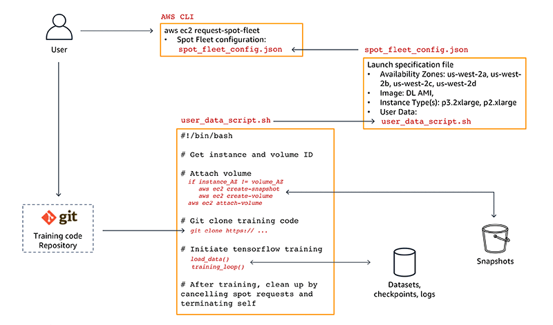
Figure 3: Data, code and configuration artifacts dependency chart

Let’s start with you, the user.

As a deep learning researcher or developer, first prototype and develop your models locally or on an inexpensive CPU-only Amazon EC2 on-demand instance with the AWS Deep Learning AMI. When you’re ready to run a training job on GPUs, you then push your training scripts to a Git repository.

Next, submit a spot request using the aws ec2 request-spot-fleet command shown in step 6. This sets everything into motion.

The spot request uses the spot fleet configuration file spot_fleet_config.json to launch the desired spot instance type. In this example, you run a training job on a p3.2xlarge instance in any of the us-west-2 Region’s Availability Zones. The training script will run on an instance imaged using the AWS Deep Learning AMI, which includes GPU optimized TensorFlow framework.

The spot fleet configuration file also includes the user_data_script.sh bash script file. The user data bash script is executed on the spot instance at launch. This script is responsible for mounting the dataset and checkpoint volume, cloning the training scripts, and initiating the training as we saw in step 3.

In the event of a spot interruption due to higher spot instance price or lack of capacity, the instance will be terminated and the dataset and checkpoints Amazon EBS volume will be detached. Spot fleet then places another request to automatically replenish the interrupted instance.

When the request is fulfilled again, a new spot instance will be launched and it will execute the user_data_script.sh at launch. The script queries for the dataset and checkpoint volume. If the volume and the instance are in different Availability Zones, it first creates a snapshot of the volume and then creates a new volume based on the snapshot in the current instance’s Availability Zone. The volume in the previous Availability Zone is deleted to ensure there is only one source of truth.

The script then attaches the volume to the instance and resumes training from the most recent checkpoint. Once training is complete the spot fleet request is cancelled and the current running instance is terminated.

If you want to specify a higher maximum spot instance price, or change instance types or Availability Zones, simply cancel the running spot fleet request by issuing aws ec2 cancel-spot-fleet-requests and initiating a new request with an updated spot fleet configuration file spot_fleet_config.json

Summary

That’s your overview about how spot instances can be used to run deep learning training experiments on GPU instances at a much lower cost than on-demand instances.

The setup in this blog post can be extended to cover more advanced deep learning workflows, and here are some ideas:

• Multi-GPU training. Update the training script to enable multi-GPU training
• Sub-epoch granularity checkpointing and resuming. In this example, checkpoints are saved only at the end of each epoch. For large datasets and complex models that take long time to finish an epoch, frequent checkpointing minimizes progress loss during interruption.
• Multiple parallel experiments. Increase spot fleet target capacity to run multiple independent training jobs with different hyperparameters.

I hope you enjoyed reading this post. If you have questions, comments or feedback please use the comments section below. Happy spot training!

About the Author

Shashank Prasanna is an AI & Machine Learning Technical Evangelist at Amazon Web Services (AWS) where he focuses on helping engineers, developers and data scientists solve challenging problems with machine learning. Prior to joining AWS, he worked at NVIDIA, MathWorks (makers of MATLAB & Simulink) and Oracle in product marketing, product management, and software development roles.

Amazon Elastic Inference (Amazon EI) is a service that allows you to attach low-cost GPU-powered acceleration to Amazon EC2 and Amazon SageMaker instances. MXNet has supported Amazon EI since its initial release at AWS re:Invent 2018.

In this blog post, we’ll explore the cost and performance benefits of using Amazon EI with MXNet. We’ll walk you through an example that shows you how we improved our initial inference latency of 43ms by 1.69x, and how we improved cost efficiency by 75 percent.

The benefits of Amazon Elastic Inference

Amazon Elastic Inference can reduce the cost of running deep learning inference by up to 75 percent. First let’s take a look at how Elastic Inference compares to other Amazon EC2 options in terms of performance and cost.

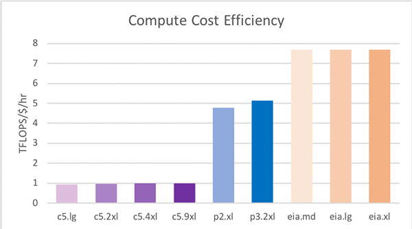
The table below lists the specific details for each EC2 option, in terms of resources, capacity and cost. Note that the c5.xlarge plus eia1.xlarge has a similar amount of compute capacity as a p2.xlarge (see the two highlighted rows in the table below).

If we look at the compute capability (Tera-Floating-point-Operations-Per-Second, or TFLOPS) a C5.4XLarge provides 0.67 TFLOPS of performance for $0.68 an hour, whereas an EIA1.Medium with 1.00 TFLOPS costs just $0.13 per hour. If pure performance (ignoring costs) is the goal, clearly leveraging a P3.2XLarge instance will provide the most compute at 15.7 TFLOPS. But in the last column showing TFLOPS per dollar we see that the EI accelerators (EIA) provide the most value. Since EI accelerators (EIA) must be attached to an EC2 instance, the last row shows one possible combination. The C5.XLarge plus the EIA1.XLarge has a similar amount of vCPUs and TFLOPS as a P2.XLarge, but the cost per hour of the C5XLarge plus the EIA1.XLarge is $0.69 per hour compared with $0.90 per hour for the P2.XLarge. That’s a $0.21 per hour discount. This highlights the other benefit of using Amazon EI which is being able to configure the amount of vCPUs, memory, and GPU compute to match your needs.

Using Apache MXNet with Amazon EI

Apache MXNet is an open source deep learning framework used to build, train, and deploy deep neural networks. MXNet abstracts much of the complexity involved in implementing neural networks, is highly performant and scalable, and offers APIs across popular programming languages such as Python, C++, Java, R, Scala, and more. Amazon EI enabled Apache MXNet is available in the AWS Deep Learning AMI. A ‘pip’ package is also available on Amazon S3 so you can build it in to your own Amazon Linux or Ubuntu AMIs, or Docker containers.

Now we’ll analyze the performance (latency) and cost efficiency trade-offs for a ResNet-152 model for various instances. We’ll start with this example code from AWS and modify it for this blog post. The changes required to measure inference performance are in blue below:

import time
import mxnet as mx
import numpy as np
from collections import namedtuple
Batch = namedtuple('Batch', ['data'])

#download model files and labels
path='http://data.mxnet.io/models/imagenet/'
[mx.test_utils.download(path+'resnet/152-layers/resnet-152-0000.params'),
mx.test_utils.download(path+'resnet/152-layers/resnet-152-symbol.json'),
mx.test_utils.download(path+'synset.txt')]

#set the context to run inference with
ctx = mx.eia()

#load the model from file and configure
sym, arg_params, aux_params = mx.model.load_checkpoint('resnet-152', 0)
mod = mx.mod.Module(symbol=sym, context=ctx, label_names=None)
mod.bind(for_training=False, data_shapes=[('data', (1,3,224,224))],
     label_shapes=mod._label_shapes)
mod.set_params(arg_params, aux_params, allow_missing=True)
with open('synset.txt', 'r') as f:
  labels = [l.rstrip() for l in f]

#download the image from file and convert into format (batch, RGB, width, height)
fname = mx.test_utils.download('https://github.com/dmlc/web-data/blob/master/mxnet/doc/tutorials/python/predict_image/cat.jpg?raw=true')
img = mx.image.imread(fname)
img = mx.image.imresize(img, 224, 224) # resize
img = img.transpose((2, 0, 1)) # Channel first
img = img.expand_dims(axis=0) # batchify

first = -1
sum = 0
runs = 100
for iter in range(runs):
    start = time.time()
    #run inference
    mod.forward(Batch([img]))
    prob = mod.get_outputs()[0].asnumpy()
    #time inference latency
    elapsed = (time.time() - start) * 1000
    if iter == 0:
        first = elapsed
    else:
        sum += elapsed
avg = sum / (runs-1)
print('First inference: %4.2f ms' % first)
print('Average inference: %4.2f ms' % avg)

You can see we added a loop around the inference call and timed the forward() and get_outputs() functions. MXNet uses lazy evaluation, so to force it to execute the forward call we need to use the outputs (by converting them to a numpy array). The first inference is abnormally slow due to initialization with the remote GPU on the EIA, so we stored the first inference time and summed the remaining inference latencies to compute an average.

Setting up an instance with an EI accelerator

We’ll launch an instance using the AWS Deep Learning AMI (DLAMI), which already provides support for Apache MXNet with Amazon EI. You can review Elastic Inference Prerequisites for the instructions related to Elastic Inference. You can review how to launch a DLAMI with an Elastic Inference Accelerator in the Elastic Inference documentation.

Testing on an instance with an EI accelerator

We launched a C5.4XLarge instance with the largest EI accelerator: EIA1.XLarge. This is probably more compute than we need but it will give us a good starting point from which to work backward from the best performance we can get with EI. Next, we activated the conda environment that was pre-installed for MXNet on EI with the following command:

source activate amazonei_mxnet_p36

Running our code on an instance with an EI accelerator produces this output:

[15:34:09] src/nnvm/legacy_json_util.cc:209: Loading symbol saved by previous version v0.8.0. Attempting to upgrade...
[15:34:09] src/nnvm/legacy_json_util.cc:217: Symbol successfully upgraded!
Using Amazon Elastic Inference Client Library Version: 1.2.12
Number of Elastic Inference Accelerators Available: 1
Elastic Inference Accelerator ID: eia-b774f0694b614549944c13dc0aa3ddc0
Elastic Inference Accelerator Type: eia1.xlarge

First inference: 2763.00 ms
Average inference: 20.34 ms

Notice that the larger first inference time is 2763.00 ms. After the first inference, the average for the other 99 iterations is 20.34 ms.

Testing on a C5 instance

We can use the same script with just one change to run inference using only the CPU on the same instance. Here MXNet won’t use the EI accelerator when we set the context to CPU:

# We’re commenting out EIA context, and instead use a CPU context
# ctx = mx.eia()
ctx = mx.cpu()

Running this code now produces this output:

[14:33:41] src/nnvm/legacy_json_util.cc:209: Loading symbol saved by previous version v0.8.0. Attempting to upgrade...
[14:33:41] src/nnvm/legacy_json_util.cc:217: Symbol successfully upgraded!
[14:33:42] src/operator/nn/mkldnn/mkldnn_base.cc:74: Allocate 147456 bytes with malloc directly
[14:33:42] src/operator/nn/mkldnn/mkldnn_base.cc:74: Allocate 589824 bytes with malloc directly
[14:33:42] src/operator/nn/mkldnn/mkldnn_base.cc:74: Allocate 2359296 bytes with malloc directly
[14:33:42] src/operator/nn/mkldnn/mkldnn_base.cc:74: Allocate 9437184 bytes with malloc directly
First inference: 1659.79 ms
Average inference: 44.61 ms

Notice that the average inference is 44.61 ms. Compared to our initial run using the EI accelerator, the CPU takes 2.19x longer for each inference call on average when using a standard C5 instance.

Testing on GPU instances

Next, we launched a separate P2.XLarge instance to compare the performance to. We used the same DLAMI version. After the instance was launched we activated the regular MXNet conda environment:

source activate mxnet_p36

Now we need to make two more tweaks to our script:

# We’re commenting out the CPU context as well, and instead use a GPU context
# ctx = mx.eia()
# ctx = mx.cpu()
ctx = mx.gpu()

...

img = img.transpose((2, 0, 1)) # Channel first
img = img.expand_dims(axis=0) # batchify
img = img.as_in_context(mx.gpu())

The first context that we change is the one used for binding, and the second context we change is the one that defines where our input data resides. For CPU and EIA instances, data must be allocated on a CPU context. It’s important to point out that typically you create your ndarrays on the same context that you bind the model to (CPU for CPU, and GPU for GPU). But for EIA you bind your model to the EIA context. You create your data with the CPU context. MXNet automatically copies the data over as needed for EIA.

Running this code on the P2.XLarge instance now produces this output:

[14:42:07] src/nnvm/legacy_json_util.cc:209: Loading symbol saved by previous version v0.8.0. Attempting to upgrade...
[14:42:07] src/nnvm/legacy_json_util.cc:217: Symbol successfully upgraded!
[14:42:09] src/operator/nn/./cudnn/./cudnn_algoreg-inl.h:97: Running performance tests to find the best convolution algorithm, this can take a while... (setting env variable MXNET_CUDNN_AUTOTUNE_DEFAULT to 0 to disable)
First inference: 7916.36 ms
Average inference: 41.10 ms

Before we draw any conclusions, let’s launch a separate P3.2XLarge instance to compare the performance to. We can reuse the same script, DLAMI, and conda environment that we used earlier for the P2.XLarge instance. Running the code now produces this output on the P3.2XLarge instance:

[14:59:33] src/nnvm/legacy_json_util.cc:209: Loading symbol saved by previous version v0.8.0. Attempting to upgrade...
[14:59:33] src/nnvm/legacy_json_util.cc:217: Symbol successfully upgraded!
[14:59:35] src/operator/nn/./cudnn/./cudnn_algoreg-inl.h:97: Running performance tests to find the best convolution algorithm, this can take a while... (setting env variable MXNET_CUDNN_AUTOTUNE_DEFAULT to 0 to disable)
First inference: 1911.22 ms
Average inference: 12.31 ms

Comparing C5, P2, P3, and EIA instances

Plotting the data we’ve collected thus far we can see that GPU performed better than CPU (as expected) and the V100 GPU in P3 instances is 3.34x faster than the K80 GPU in P2 instances. Where before you had to choose between P2 and P3, now EI gives you another choice in between with a 2.02x increase in speed over P2.

Based purely on instance cost per hour (in us-east-1 for EIA and EC2) we can see that the cost for the C5.4XL + EIA.XL is in between the costs for the P2 and P3 instances (see the following table). However, when factoring the cost to perform 100,000 inferences we can see that the P2 and P3 instances have similar costs, and the C5.4XL and the C5.4XL +EI instances are also within a penny of each other ($0.84 and $0.83). The big picture here is that by using EIA we get better than P2 performance at the cost of a C5 instance. What a deal!

Exploring all possibilities

Now, let’s do more investigation and try out additional instance combinations for EI. After rerunning the initial script we started with on combinations of C5.Large, C5.XLarge, C5.2XLarge, and C5.4XLarge with EI accelerators EIA1.Medium, EIA1.Large, and EIA1.XLarge we produced the latest table:

In this table, when we look at the host instance types with the EIA1.Medium (yellow highlight) we see similar results. This means that there isn’t a lot of host-side processing, so going to a larger host instance doesn’t improve performance. This indicates to us that we can save on cost by choosing a smaller instance. Similarly, looking at host instances with all using the largest EIA1.XLarge accelerator (blue highlight) there isn’t a noticeable performance difference either. This confirms that EIA performance isn’t limited by the size of the host either. It also means that we can continue to use the C5.Large host instance type, achieve the same performance, and pay less.

Comparing inference latency

Now that we’ve decided on a C5.Large host instance type, we can look at the accelerator types. There is a progression from 39.18ms to 25.90ms and finally to 20.34ms in terms of inference latency. The following chart shows what we get if we add our new data points for the various accelerator sizes to our previous chart:

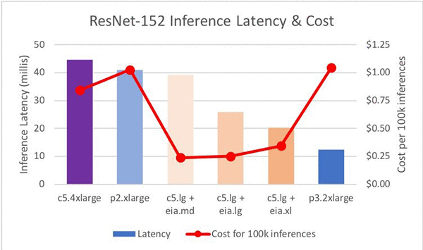
This chart shows that the EI accelerators provide a set of steps between P2 and P3 in terms of raw performance.

Comparing inference cost efficiency

The last column in the table shows the cost efficiency of the combination. Reviewing this column we see that the C5.Large + EIA1.Medium has the best cost efficiency. In a pure least-cost comparison, the C5.Large + EIA1.Medium combination provides the best cost efficiency when compared to the C5.4XL and the P2/P3 instances. Savings are  71 percent to 77 percent. And the C5.Large + EIA1.XLarge provides a 2.02x increase in speed over a P2 and a 2.19x speedup over the C5.4XL (CPU only). The savings are 66 percent and 59 percent, respectively.

Conclusions

Here’s what we’ve found so far:

• Combining EI accelerators with any host instance type enables users to choose the amount of host compute, memory, etc. with a configurable amount of GPU memory and compute.
• EI accelerators provide a range of memory and compute that is similar to P2 instances, but with a lower cost
• EI accelerators can bridge the gap in terms of raw performance (inference latency) between P2 and P3 instance types.
• EI accelerators can achieve a better cost efficiency than C5 and P2/P3 instances.

In our analysis we found that the ease of use in MXNet is as simple as changing the context for binding a model and ndarray creation. This allowed us to use largely the same test script on CPU, GPU, and EIA contexts in MXNet, and ease our testing and performance analysis.

We started with a Resnet-152 model running on a C5.4XLarge instance with a 44ms inference latency. We reduced it to 20ms by migrating to a C5.Large + EIA.XLarge.  This resulted in a 2.19x increase in speed with a $0.07 hourly cost savings to top it off. We also found that we could achieve a 71 percent cost savings ($0.84versus $0.24 per 100k inferences) with a C5.Large + EIA.Medium and still get better performance (44ms versus 39ms).

Call to Action

Try out MXNet on EI and see how much you can save while still improving performance for inference on your model. Here are the steps we went through to analyze the design space for deep learning inference, and you can follow these steps for your model:

1. Write a test script to analyze inference performance for CPU context.
2. Create copies of the script with tweaks for GPU and EIA contexts.
3. Run scripts on C5, P2, and P3 instance types to get a baseline for performance.
4. Analyze the performance of EIA.
   1. Start with largest EI accelerator type and a large host instance type.
   2. Work backward until you find a combo that is too small.
5. Introduce cost efficiency to the analysis by computing the cost to perform 100k inferences.

How much can you save while still improving the performance of inference for your model? How fast can you improve the inference latency of your model without spending a single cent more? Share your results in the comments section.

About the Authors

Sam Skalicky is a Software Engineer with AWS Deep Learning and enjoys building heterogeneous high performance computing systems. He is an avid coffee enthusiast and avoids hiking at all costs.

Hagay Lupesko is an Engineering Manager for AWS Deep Learning. He focuses on building Deep Learning tools that enable developers and scientists to build intelligent applications. In his spare time he enjoys reading, hiking and spending time with his family.