Hey everyone, I was wondering if there were any resources on how to fine-tune GPT-2 on a custom corpus of data, for example, Shakespearean poems or Cornell Movie Dialogues.
My name is Dima and I wanted to tell you about an open-source library we work on called TamnunML.
Our goal is to provide an easy to use library (with sklearn interface) for complex model training and fine-tuning. For example, with tamnun you can train any pytorch module like this:
“`python from torch import nn from tamnun.core import TorchEstimator
or, you can fine tune BERT on your task as easy as: “`python from tamnun.bert import BertClassifier, BertVectorizer from sklearn.pipeline import make_pipeline
Let’s say we have an N-class semantic segmentation problem. Now on each iteration (for each batch) we can calculate Dice loss in two ways: (1) calculate average loss over classes for each sample in a batch and after that get the average over batch, or (2) calculate average loss per class in a batch and then average over classes presented in a batch. Which one is better and why? Or there is no difference at all? Can it affect on how model learns to segment small or big objects? Any related articles?
We are working on a tool, which is supposed to help developers test, understand and explain their machine learning models. The tool will be open-source and free to use.
We are in the prototyping stage and have a prototype ready to show. If anyone would like to have a look and give us feedback, that would be awesome!
If you have experience with testing models and frameworks like SHAP and LIME, it would be even more valuable.
Hello guys! I’m training GRU neural network with single GRU layer (among other layers), and I tend to think that hidden to hidden transformation requires severe non-linearity to correctly “merge” memory with current timestep (and thus update hidden). How do I approach this, what is the best practice? Should I add more GRU layers or should I, for instance, add extra layers to hidden to hidden transformation with nonlinearity like relu? If I take second approach I guess I should use tanh instead of relu to avoid exploding gradients, am I correct?
When I came across Customer Support on Twitter dataset, I couldn’t help but wanted to model and compare airlines customer service twitter response time.
I wanted to be able to answer questions like:
Are there significant differences on customer service twitter response time among all the airlines in the data?
Is the weekend affect response time?
Do longer tweets take longer time to respond?
Which airline has the shortest customer service twitter response time and vice versa?
The data
It is a large dataset contains hundreds of companies from all kinds of industries. The following data wrangling process will accomplish:
Get customer inquiry, and corresponding response from the company in every row.
Convert datetime columns to datetime data type.
Calculate response time to minutes.
Select only airline companies in the data.
Any customer inquiry that takes longer than 60 minutes will be filtered out. We are working on requests that get response in 60 minutes.
plt.figure(figsize=(10,5))
sns.distplot(df['response_time'], kde=False)
plt.title('Frequency of response by response time')
plt.xlabel('Response time (minutes)')
plt.ylabel('Number of responses');
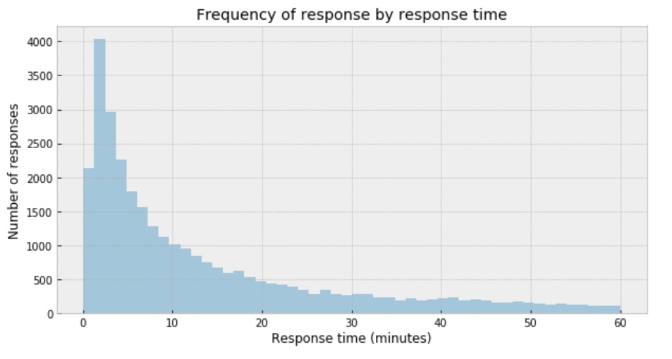
Figure 1
My immediate impression is that a Gaussian distribution is not a proper description of the data.
Student’s t-distribution
One useful option when dealing with outliers and Gaussian distributions is to replace the Gaussian likelihood with a Student’s t-distribution. This distribution has three parameters: the mean (𝜇), the scale (𝜎) (analogous to the standard deviation), and the degrees of freedom (𝜈).
Set the boundaries of the uniform distribution of the mean to be 0 and 60.
𝜎 can only be positive, therefore use HalfNormal distribution.
set 𝜈 as an exponential distribution with a mean of 1.
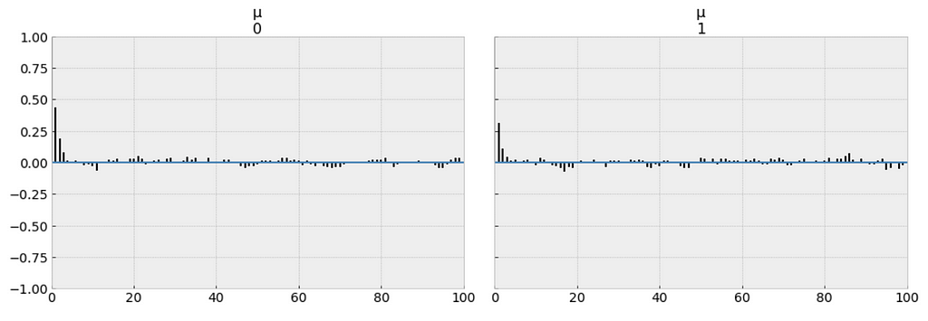
From the following trace plot, we can visually get the plausible values of 𝜇 from the posterior.
We should compare this result with those from the the result we obtained analytically.
az.plot_trace(trace_t[:1000], var_names = ['μ']);
Figure 2
df.response_time.mean()
The left plot shows the distribution of values collected for 𝜇. What we get is a measure of uncertainty and credible values of 𝜇 between 7.4 and 7.8 minutes.
It is obvious that samples that have been drawn from distributions that are significantly different from the target distribution.
Posterior predictive check
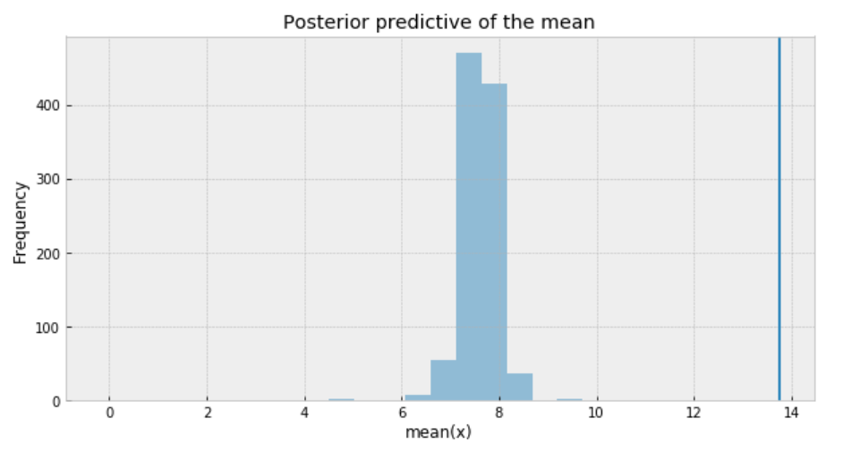
One way to visualize is to look if the model can reproduce the patterns observed in the real data. For example, how close are the inferred means to the actual sample mean:
ppc = pm.sample_posterior_predictive(trace_t, samples=1000, model=model_t)
_, ax = plt.subplots(figsize=(10, 5))
ax.hist([n.mean() for n in ppc['y']], bins=19, alpha=0.5)
ax.axvline(df['response_time'].mean())
ax.set(title='Posterior predictive of the mean', xlabel='mean(x)', ylabel='Frequency');
Figure 3
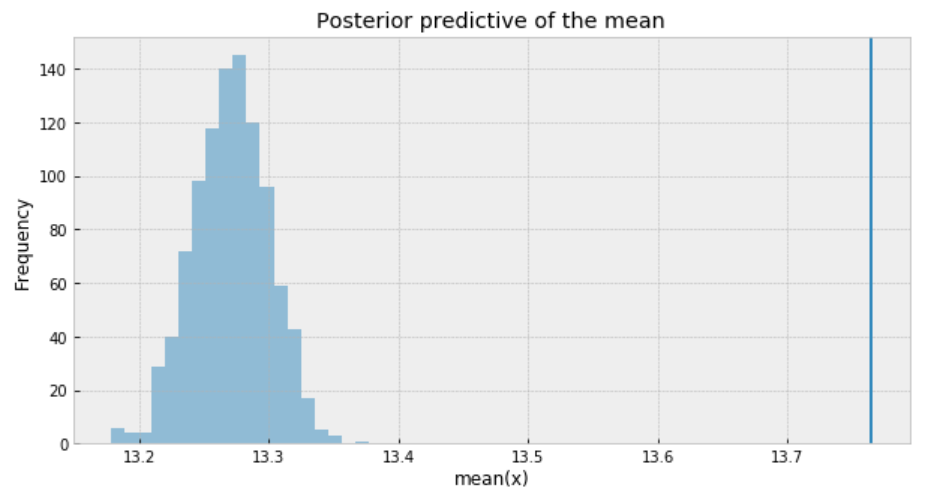
The inferred mean is so far away from the actual sample mean. This confirms that Student’s t-distribution is not a proper choice for our data.
Poisson distribution
Poisson distribution is generally used to describe the probability of a given number of events occurring on a fixed time/space interval. Thus, the Poisson distribution assumes that the events occur independently of each other and at a fixed interval of time and/or space. This discrete distribution is parametrized using only one value 𝜇, which corresponds to the mean and also the variance of the distribution.
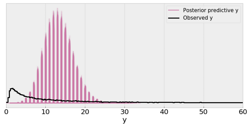
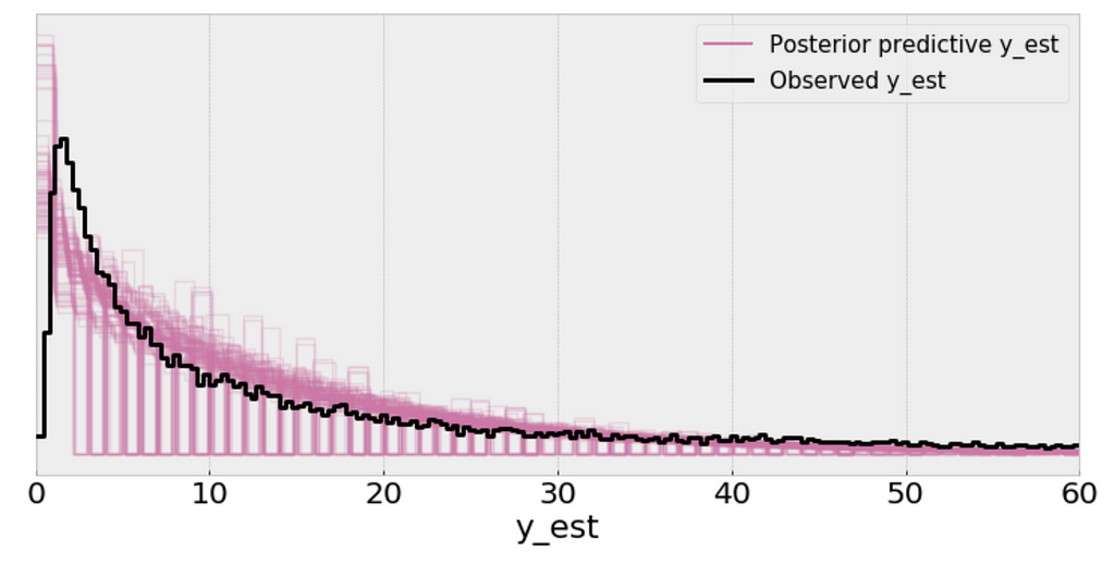
The single (black) line is a kernel density estimate (KDE) of the data and the many purple lines are KDEs computed from each one of the 100 posterior predictive samples. The purple lines reflect the uncertainty we have about the inferred distribution of the predicted data.
From the above plot, I can’t consider the scale of a Poisson distribution as a reasonable practical proxy for the standard deviation of the data even after removing outliers.
Posterior predictive check
ppc = pm.sample_posterior_predictive(trace_p, samples=1000, model=model_p)
_, ax = plt.subplots(figsize=(10, 5))
ax.hist([n.mean() for n in ppc['y']], bins=19, alpha=0.5)
ax.axvline(df['response_time'].mean())
ax.set(title='Posterior predictive of the mean', xlabel='mean(x)', ylabel='Frequency');
Figure 7
The inferred means to the actual sample mean are much closer than what we got from Student’s t-distribution. But still, there is a small gap.
The problem with using a Poisson distribution is that mean and variance are described by the same parameter. So one way to solve this problem is to model the data as a mixture of Poisson distribution with rates coming from a gamma distribution, which gives us the rationale to use the negative-binomial distribution.
Negative binomial distribution
Negative binomial distribution has very similar characteristics to the Poisson distribution except that it has two parameters (𝜇 and 𝛼) which enables it to vary its variance independently of its mean.
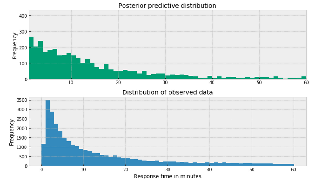
Using the Negative binomial distribution in our model leads to predictive samples that seem to better fit the data in terms of the location of the peak of the distribution and also its spread.
Posterior predictive check
ppc = pm.sample_posterior_predictive(trace_n, samples=1000, model=model_n)
_, ax = plt.subplots(figsize=(10, 5))
ax.hist([n.mean() for n in ppc['y_est']], bins=19, alpha=0.5)
ax.axvline(df['response_time'].mean())
ax.set(title='Posterior predictive of the mean', xlabel='mean(x)', ylabel='Frequency');
Figure 10
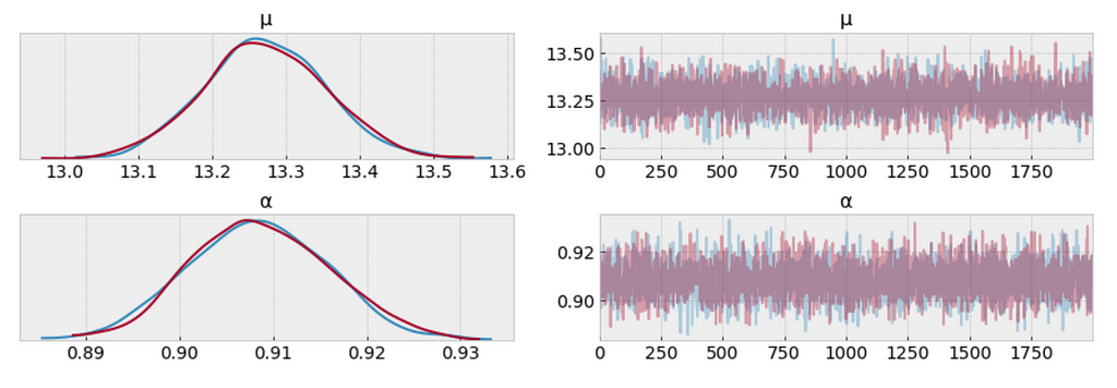
To sum it up, the following are what we get for the measure of uncertainty and credible values of (𝜇):
Student t-distribution: 7.4 to 7.8 minutes
Poisson distribution: 13.22 to 13.34 minutes
Negative Binomial distribution: 13.0 to 13.6 minutes.
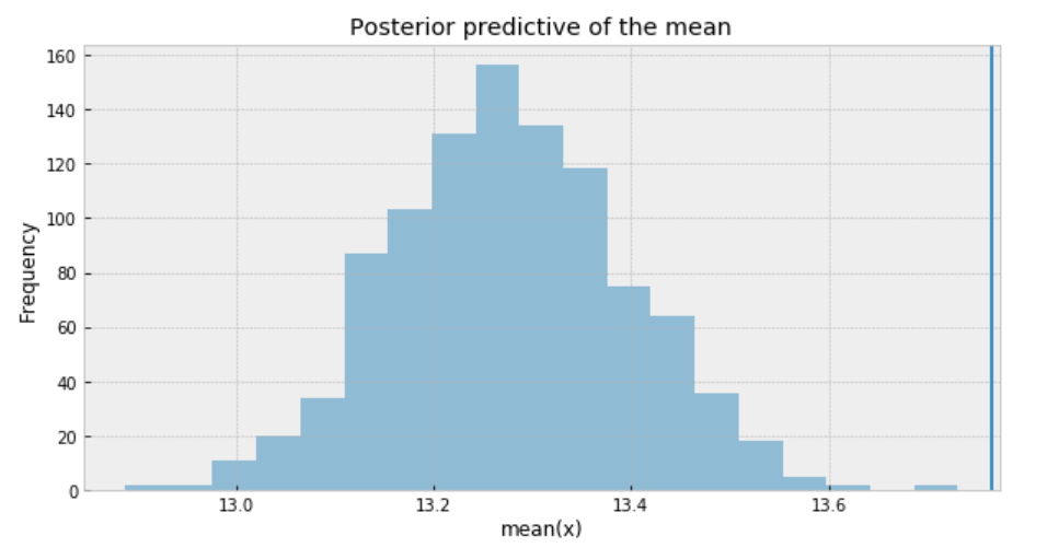
The posterior predictive distribution somewhat resembles the distribution of the observed data, suggesting that the Negative binomial model is a more appropriate fit for the underlying data.
Bayesian methods for hierarchical modeling
We want to study each airline as a separated entity. We want to build a model to estimate the response time of each airline and, at the same time, estimate the response time of the entire data. This type of model is known as a hierarchical model or multilevel model.
My intuition would suggest that different airline has different response time. The customer service twitter response from AlaskaAir might be faster than the response from AirAsia for example. As such, I decide to model each airline independently, estimating parameters μ and α for each airline.
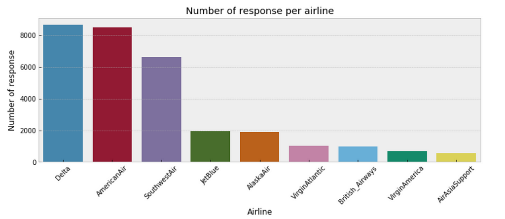
One consideration is that some airlines may have fewer customer inquiries from twitter than others. As such, our estimates of response time for airlines with few customer inquires will have a higher degree of uncertainty than airlines with a large number of customer inquiries. The below plot illustrates the discrepancy in sample size per airline.
plt.figure(figsize=(12,4))
sns.countplot(x="author_id_y", data=df, order = df['author_id_y'].value_counts().index)
plt.xlabel('Airline')
plt.ylabel('Number of response')
plt.title('Number of response per airline')
plt.xticks(rotation=45);
Figure 12
Bayesian modeling each airline with negative binomial distribution
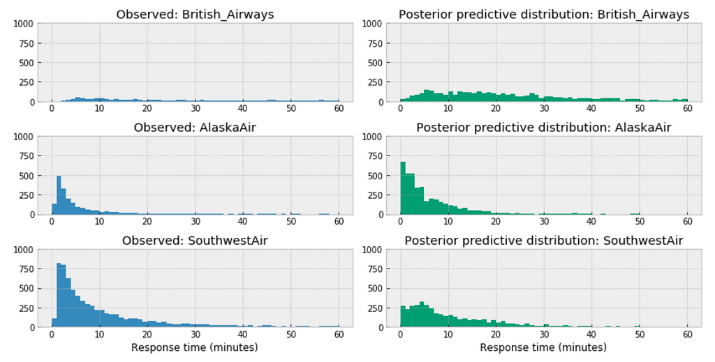
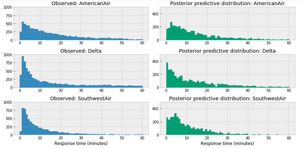
Among the above three airlines, British Airways’ posterior predictive distribution vary considerably to AlaskaAir and SouthwestAir. The distribution of British Airways towards right.
This could accurately reflect the characteristics of its customer service twitter response time, means in general it takes longer for British Airways to respond than those of AlaskaAir or SouthwestAir.
Or it could be incomplete due to small sample size, as we have way more data from Southwest than from British airways.
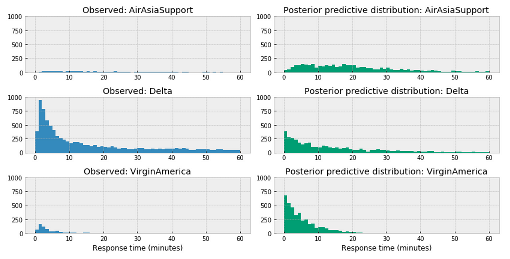
Similar here, among the above three airlines, the distribution of AirAsia towards right, this could accurately reflect the characteristics of its customer service twitter response time, means in general, it takes longer for AirAsia to respond than those of Delta or VirginAmerica. Or it could be incomplete due to small sample size.
For the airlines we have relative sufficient data, for example, when we compare the above three large airlines in the United States, the posterior predictive distribution do not seem to vary significantly.
Bayesian Hierarchical Regression
The variables for the model:
df = df[['response_time', 'author_id_y', 'created_at_y_is_weekend', 'word_count']]
formula = 'response_time ~ ' + ' + '.join(['%s' % variable for variable in df.columns[1:]])
formula
In the following code snippet, we:
Convert categorical variables to integer.
Estimate a baseline parameter value 𝛽0 for each airline customer service response time.
Estimate all the other parameter across the entire population of the airlines in the data.
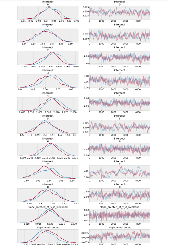
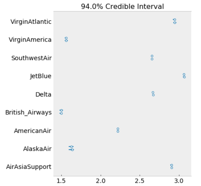
The model estimates the above β0 (intercept) parameters for every airline. The dot is the most likely value of the parameter for each airline. It look like our model has very little uncertainty for every airline.
I am currently doing a literature search of sparse training architectures, I am thinking of making a library for sparse training and hoping to make it as universal as possible. For that, I would need to get a good idea for the various use cases.
I’m interested in transitioning from web development to machine learning.
My math background is mediocre (basic calc) and my only programming experience is in web dev technologies (3 years). I want to be realistic about my effort level and opportunities. I probably won’t be going back to college, but have 10 months left on a work contract and would like to spend any free time learning the basics.
What is the feel of competition in the field? With my time-frame and background, is it reasonable to think I can earn an entry-level position?
I’ve heard the field is broken up into data science and data modeling. Is data modeling more programmatic? Will my experience as a dev be more relevant there?