It all started at a startup summit I visited. There I thought of teaching an AI to generate start-up ideas.
I couldn’t find data, so I decided to make it generate start-up news from TechCrunch.
I decided this would be a good time to test GPT-2, which generated believable outputs.
I trained this network using Google Colab, since my ML machine has no GPU and a bad CPU.
Anyway, here are the results!
Prompt: “funding”
s’ 26/“Fitz Frames is planning on giving away pairs of goggles as an homage to the brand, 27/ Stella Brands has revealed it has had an ownership stake in Fitz Frames since 2012 Rex 28/ with Marco Benevento is the birth name of the latest wave of millennial investors Y Combinator 39/ Star Wars Celebration Star Wars Celebration Fitz Frames is currently active on Y Combinator’s fundraising page, raising $15 million in seed funding and several more round funding rounds. Its fourth round is set to be its last, in early 2017, bringing its valuation to between $50 and $100 million, as it attempts to resuscitate the increasingly popular glasses. Fitz Frames hopes to become a more durable, lightweight option for travel, and is pursuing businesses that share its technology with bring the option of attaching sunglasses to people’s feet. It stems from a game where two friends play jack-of-all-trades, attempting to become the first to have their glasses replaced. While other players in the jack-of-all-trades game have tried to make it to the final round, in which the winner is determined by best results from the next round. Players toss duct tape over their faces to make room for new glasses, and drop them somewhere cool for future decorating. The game is currently in its fourth season, and said fourth round will be its biggest to date, with all-new glasses added by the day. A new website is hoping to get around this by giving players a more standardized format for making their purchases. It’s called Lux, and it’s set to’ inspiration’be”ite consumers. “The way we think about technology is related to 1) what we are able to buy and 2) what we are able to want from the experience. If you have me walk you through the steps of making a new pair of glasses, I promise you that that’s it.” Making new glasses is kind of like making your first pair of shoes, but you can’t replace the pair you got from the size chart on the website. 2) That’s the problem.” You can probably make the case for creating greater accessibility in the least,” Kiss 101 founder and CEO Gabrielle Esposito tells me. “There are tons of opportunities out there. From helping you find a bus stop to helping make your child’s doctor
Prompt: “virtual reality”
“From a physical standpoint I think the physical world is actually kind of the only guide”sarasin” about’ 14 ” with “little’� to none guidances,” added Binks. Most of us, by now, are aware that virtual reality (VR) can be a bit heavy for a country like India, where the current model focuses on physically reaching and leaving virtual walls. The problem is that there isn’t much physical speed at which a user can experience a place ‘‘.” That “b’alls of a city are a walk in the park right now, but they often aren’t possible in South Asia, where walking and running are the norm. Sri Lanka is an alternate model for India, focusing on smaller, backpack-accessible cities that don’t rely on long lines to get by, and are often hard for Asian cities like Japan and the U.S. to get their cities out of the city. In’hibited by the physical and economic advantages of the Indian subcontinent, Binks is’t seeking funding — and in this day and age of artificial intelligence and artificial deadlines, it’s crucial that governments prioritize proven methods of achieving long-term solutions. “We need to be able to rely on the cards and the the thesles,’ pondering pal Jain Cheung, co-founder and CEO of DeepMind. “We need to be able to rely on our bank and have it tell us what’s happening online,’ Cheung said. In addition to launching treating surroundings as if they were holograms, the founders’ latest approach is also use virtual reality as an alternative to the human brain for assessing long-distance travel. For now, though, the focus is on using virtual reality to help make smarter batteries — and connect-and-disconnect sensors — that our bodies have built into our’ brains. “The amount of power we have is going to have an effect on the way we do it.” said FitzGerald. “But from a health and security perspective,” said Cheung. The goal is for the technology to be applied across all healthcare services,” said Feridranco. “Any healthcare organization would like to have accurate healthcare data,” he said. “The problem is that
At DEEP conference, Advisory meetings, etc). Understanding of smart cities, automated decision-making and AI is considered an asset. From LocalWorkBC.ca – Sun, 18 Aug 2019 10:41:39 GMT – View all Toronto, ON jobs
We gather from streaming twitter, crawling hardcoded cryptocurrency telegram groups and Reddit. And we store in Elasticsearch as a single index. We trained 1/4 layers BERT MULTILANGUAGE (200MB-ish, originally 700MB-ish) released by Google on most-possible-found sentiment data on the internet, leveraging sentiment on multilanguages, eg, english, korea, japan. Actually, it is very hard to found negative sentiment related to bitcoin / btc in large volume.
s = s.filter( 'query_string', default_field = 'text', query = 'bitcoin OR btc', )
We only do text query only contain bitcoin or btc.
Consensus introduction
We have 2 questions here when saying about consensus, what happened,
to future price if we assumed future sentiment is really positive, near to 1.0 . Eg, suddenly China want to adapt cryptocurrency and that can cause huge requested volumes.
to future price if we assumed future sentiment is really negative, near to 1.0 . Eg, suddenly hackers broke binance or any exchanges, or any news that caused wreck by negative sentiment.
So, we use deep-learning to simulate for us! I use CNN-Seq2Seq architecture this time, not required to bring last memory last RNN and fast to train.
Step
We pulled last 100 hours data and aggregated every 20 minutes, Split the dataset to train and test. Test size is last 10 hours (30 datapoints, 3 * 10), and early remaining use to train.
Initiate the model and train the model by 200 epochs. learning_rate is very sensitive, I found 1e-3 is perfect. Here I never tried to do hyperparameters searching.
The model learn, if positive and negative sentiments increasing, both will increase the price. That is why, using positive consensus or negative consensus caused price going up.
Volatility of price is higher if negative sentiment is higher, still positive volatility.
Momentum of price is higher if negative sentiment is higher, still positive momentum.
Even predicted trends are far from actual test trend, for me, it quite fascinating because I can simulate the models by N times to get different variances and from here I can calculate VaR, potential volatilities and momentums, trading ratios and etc. Well, if forecasted trends follow really close with actual test trend, do not believe it too much, there is no such model able to simulate stochastic trend that depends on a lot of real world parameters.
If you remember, the purpose of the data set is to build a model that automatically suggests the right price for any given product for Mercari website sellers. I am here to attempt to see whether we can solve this problem by Bayesian statistical methods, using PyStan.
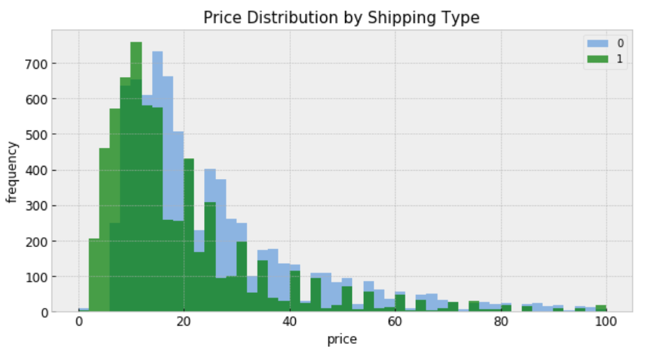
In this analysis, we will estimate parameters for individual product price that exist within categories. And the measured price is a function of the shipping condition (buyer pays shipping or seller pays shipping), and the overall price.
At the end, our estimate of the parameter of product price can be considered a prediction.
Simply put, the independent variables we are using are: category_name & shipping. And the dependent variable is: price.
from scipy import stats
import arviz as az
import numpy as np
import matplotlib.pyplot as plt
import pystan
import seaborn as sns
import pandas as pd
from theano import shared
from sklearn import preprocessing
plt.style.use('bmh')
To make things more interesting, I will model all of these 689 product categories. If you want to produce better results quicker, you may want to model the top 10 or top 20 categories, to start.
“shipping = 0” means shipping fee paid by buyer, and “shipping = 1” means shipping fee paid by seller. In general, price is higher when buyer pays shipping.
Modeling
For construction of a Stan model, it is convenient to have the relevant variables as local copies — this aids readability.
category: index code for each category name
price: price
category_names: unique category names
categories: number of categories
log_price: log price
shipping: who pays shipping
category_lookup: index categories with a lookup dictionary
There are two conventional approaches to modeling price represent the two extremes of the bias-variance tradeoff:
Complete pooling:
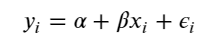
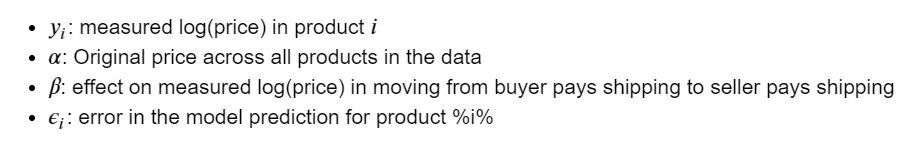
Treat all categories the same, and estimate a single price level, with the equation:
To specify this model in Stan, we begin by constructing the data block, which includes vectors of log-price measurements (y) and who pays shipping covariates (x), as well as the number of samples (N).
Once the fit has been run, the method extract and specifying permuted=True extracts samples into a dictionary of arrays so that we can conduct visualization and summarization.
We are interested in the mean values of these estimates for parameters from the sample.
b0 = alpha = mean price across category
m0 = beta = mean variation in price with change on who pays shipping
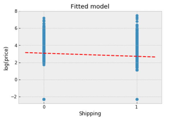
We can now visualize how well this pooled model fits the observed data.
The fitted line runs through the centre of the data, and it describes the trend.
However, the observed points vary widely about the fitted model, and there are multiple outliers indicating that the original price varies quite widely.
We might expect different gradients if we chose different subsets of the data.
Unpooling
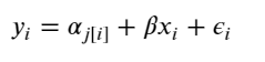
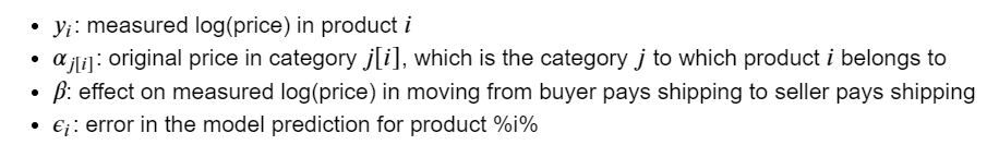
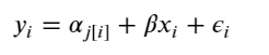
When unpooling, we model price in each category independently, with the equation:
When running the unpooled model in Stan, We again map Python variables to those used in the Stan model, then pass the data, parameters and the model to Stan. We again specify 1000 iterations of 2 chains.
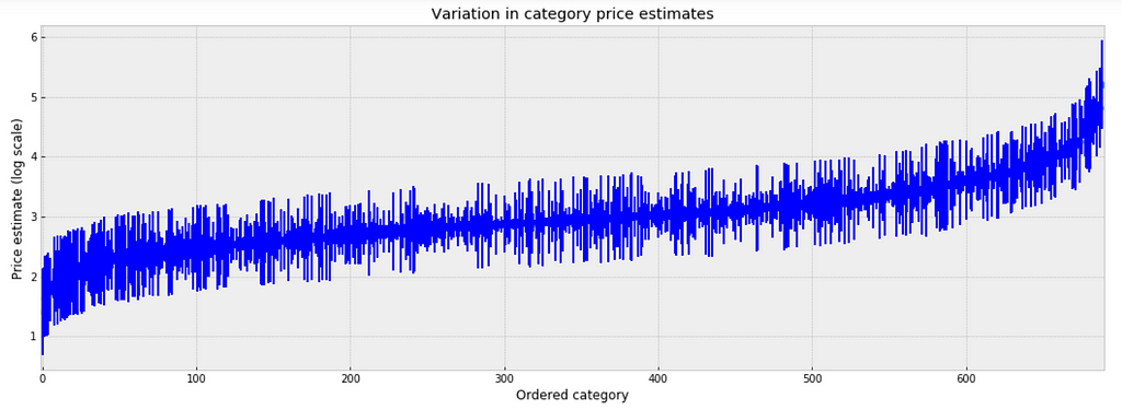
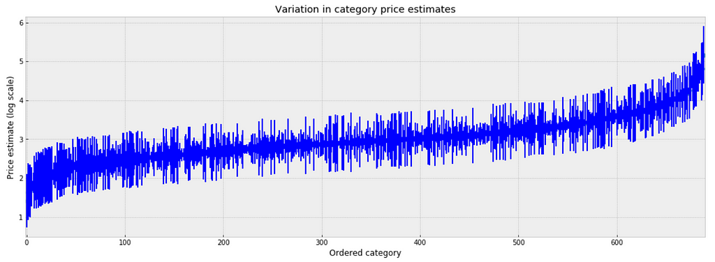
To inspect the variation in predicted price at category level, we plot the mean of each estimate with its associated standard error. To structure this visually, we’ll reorder the categories such that we plot categories from the lowest to the highest.
plt.figure(figsize=(18, 6))
plt.scatter(range(len(unpooled_estimates)), unpooled_estimates[order])
for i, m, se in zip(range(len(unpooled_estimates)), unpooled_estimates[order], unpooled_se[order]):
    plt.plot([i,i], [m-se, m+se], 'b-')
    plt.xlim(-1,690);
plt.ylabel('Price estimate (log scale)');plt.xlabel('Ordered category');plt.title('Variation in category price estimates');
Figure 4
Observations:
There are multiple categories with relatively low predicted price levels, and multiple categories with a relatively high predicted price levels. Their distance can be large.
A single all-category estimate of all price level could not represent this variation well.
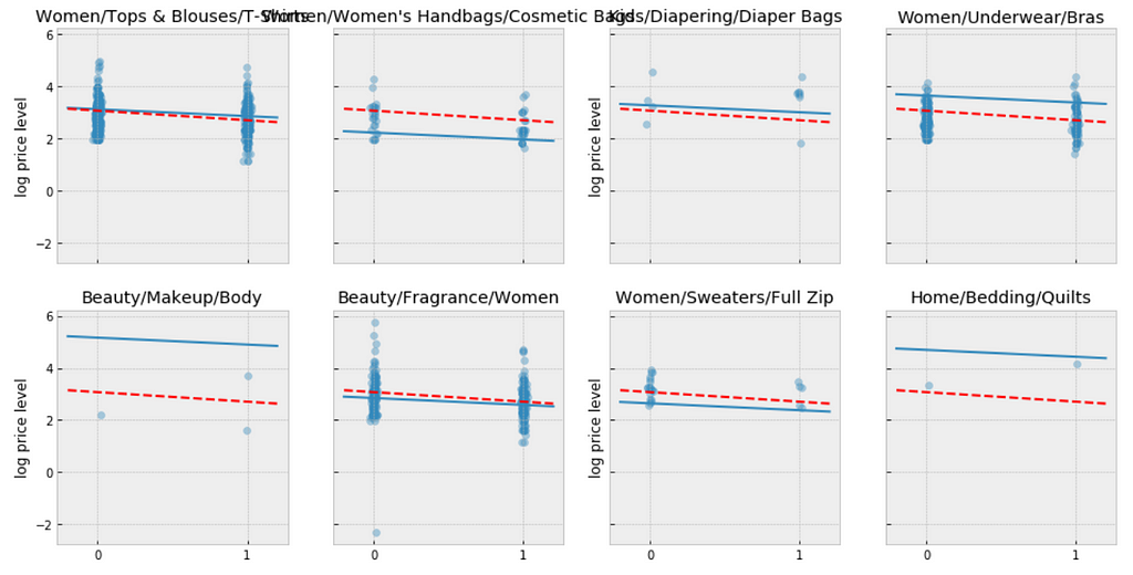
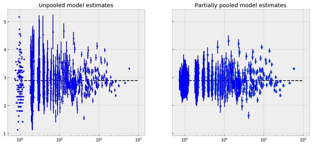
Comparison of pooled and unpooled estimates
We can make direct visual comparisons between pooled and unpooled estimates for all categories, and we are going to show several examples, and I purposely select some categories with many products, and other categories with very few products.
Let me try to explain what the above visualizations tell us:
The pooled models (red dashed line) in every category are the same, meaning all categories are modeled the same, indicating pooling is useless.
For categories with few observations, the fitted estimates track the observations very closely, suggesting that there has been overfitting. So that we can’t trust the estimates produced by models using few observations.
Multilevel and Hierarchical Models
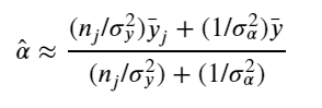
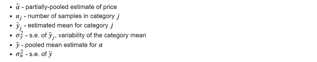
Partial Pooling — simplest
The simplest possible partial pooling model for the e-commerce price data set is one that simply estimates prices, with no other predictors (i.e. ignoring the effect of shipping). This is a compromise between pooled (mean of all categories) and unpooled (category-level means), and approximates a weighted average (by sample size) of unpooled category estimates, and the pooled estimates, with the equation:
Now we have two standard deviations, one describing the residual error of the observations, and another describing the variability of the category means around the average.
There are significant differences between unpooled and partially-pooled estimates of category-level price, The partially pooled estimates looks way less extreme.
Partial Pooling — Varying Intercept
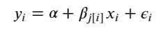
Simply put, the multilevel modeling shares strength among categories, allowing for more reasonable inference in categories with little data, with the equation:
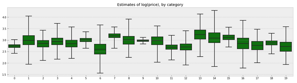
There is no way to visualize all of these 689 categories together, so I will visualize 20 of them.
a_sample = pd.DataFrame(varying_intercept_fit['a'])
plt.figure(figsize=(20, 5))
g = sns.boxplot(data=a_sample.iloc[:,0:20], whis=np.inf, color="g")
# g.set_xticklabels(df.category_name.unique(), rotation=90)  # label counties
g.set_title("Estimates of log(price), by category")
g;
Figure 7
Observations:
There are quite some variations in prices by category, and we can see that for example, category Beauty/Fragrance/Women (index at 9) with a large number of samples (225) also has one of the tightest range of estimated values.
While category Beauty/Hair Care/Shampoo Plus Conditioner (index at 16) with the smallest number of sample (one only) also has one of the widest range of estimates.
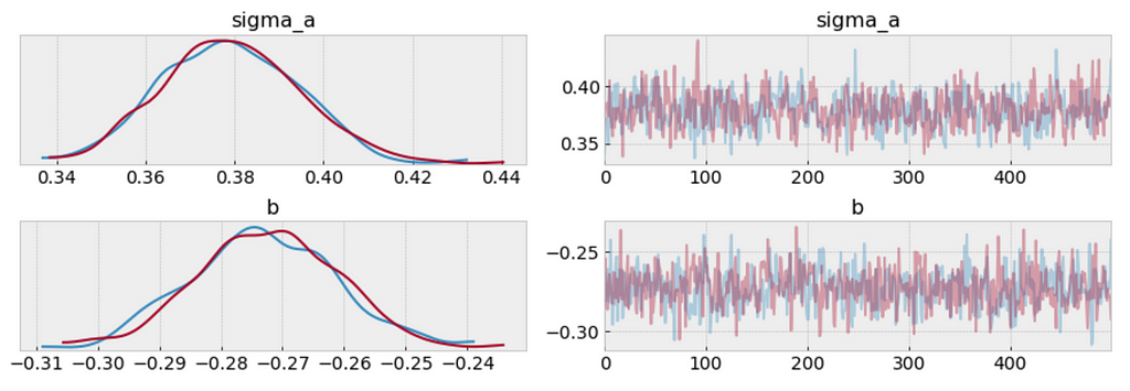
We can visualize the distribution of parameter estimates for 𝜎 and β.
The estimate for the shipping coefficient is approximately -0.27, which can be interpreted as products which shipping fee paid by seller at about 0.76 of (exp(−0.27)=0.76) the price of those shipping paid by buyer, after accounting for category.
Visualize the fitted model
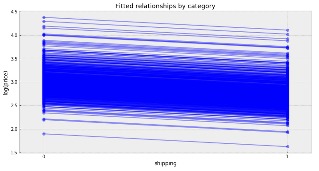
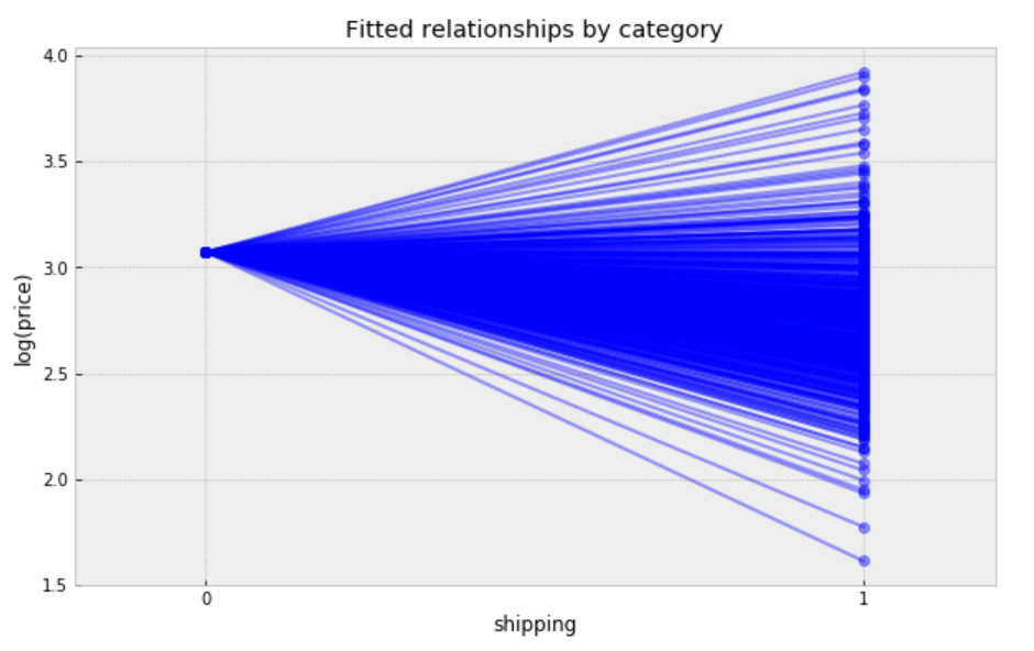
plt.figure(figsize=(12, 6))
xvals = np.arange(2)
bp = varying_intercept_fit['a'].mean(axis=0) # mean a (intercept) by category
mp = varying_intercept_fit['b'].mean()      # mean b (slope/shipping effect)
for bi in bp:
    plt.plot(xvals, mp*xvals + bi, 'bo-', alpha=0.4)
plt.xlim(-0.1,1.1)
plt.xticks([0, 1])
plt.title('Fitted relationships by category')
plt.xlabel("shipping")
plt.ylabel("log(price)");
Figure 9
Observations:
It is clear from this plot that we have fitted the same shipping effect to each category, but with a different price level in each category.
There is one category with very low fitted price estimates, and several categories with relative lower fitted price estimates.
There are multiple categories with relative higher fitted price estimates.
The bulk of categories form a majority set of similar fits.
We can see whether partial pooling of category-level price estimate has provided more reasonable estimates than pooled or unpooled models, for categories with small sample sizes.
Partial Pooling — Varying Slope model
We can also build a model that allows the categories to vary according to shipping arrangement (paid by buyer or paid by seller) influences the price. With the equation:
Following the process earlier, we will visualize 20 categories.
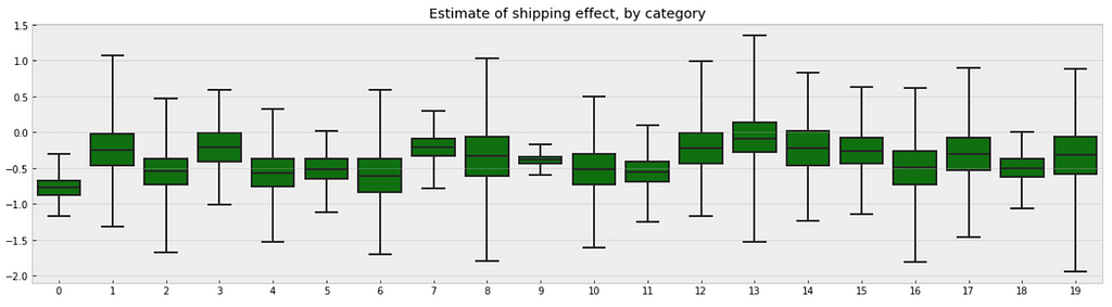
b_sample = pd.DataFrame(varying_slope_fit['b'])
plt.figure(figsize=(20, 5))
g = sns.boxplot(data=b_sample.iloc[:,0:20], whis=np.inf, color="g")
# g.set_xticklabels(df.category_name.unique(), rotation=90)  # label counties
g.set_title("Estimate of shipping effect, by category")
g;
Figure 10
Observations:
From the first glance, we may not see any difference between these two boxplots. But if you look deeper, you will find that the variation in median estimates between categories in varying slope model becomes smaller than those in varying intercept model, though the range of uncertainty is still greatest in the categories with fewest products, and least in the categories with the most products.
Visualize the fitted model:
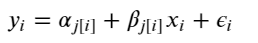
plt.figure(figsize=(10, 6))
xvals = np.arange(2)
b = varying_slope_fit['a'].mean()
m = varying_slope_fit['b'].mean(axis=0)
for mi in m:
    plt.plot(xvals, mi*xvals + b, 'bo-', alpha=0.4)
plt.xlim(-0.2, 1.2)
plt.xticks([0, 1])
plt.title("Fitted relationships by category")
plt.xlabel("shipping")
plt.ylabel("log(price)");
Figure 11
Observations:
It is clear from this plot that we have fitted the same price level to every category, but with a different shipping effect in each category.
There are two categories with very small shipping effects, but the majority bulk of categories form a majority set of similar fits.
Partial Pooling — Varying Slope and Intercept
The most general way to allow both slope and intercept to vary by category. With the equation:
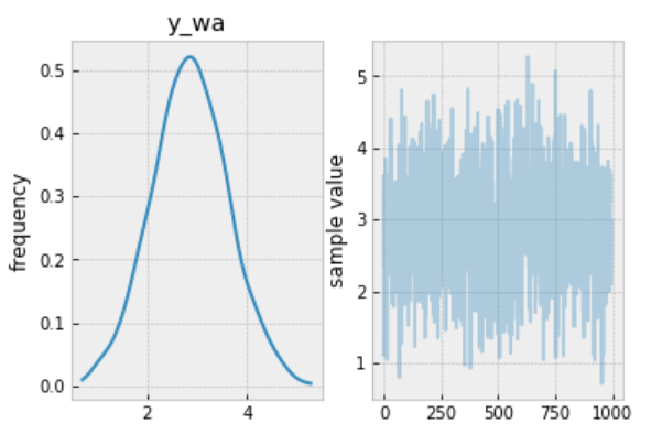
plt.figure(figsize=(10, 6))
xvals = np.arange(2)
b = varying_intercept_slope_fit['a'].mean(axis=0)
m = varying_intercept_slope_fit['b'].mean(axis=0)
for bi,mi in zip(b,m):
    plt.plot(xvals, mi*xvals + bi, 'bo-', alpha=0.4)
plt.xlim(-0.1, 1.1);
plt.xticks([0, 1])
plt.title("fitted relationships by category")
plt.xlabel("shipping")
plt.ylabel("log(price)");
Figure 12
While these relationships are all very similar, we can see that by allowing both shipping effect and price to vary, we seem to be capturing more of the natural variation, compare with varying intercept model.
Contextual Effects
In some instances, having predictors at multiple levels can reveal correlation between individual-level variables and group residuals. We can account for this by including the average of the individual predictors as a covariate in the model for the group intercept.
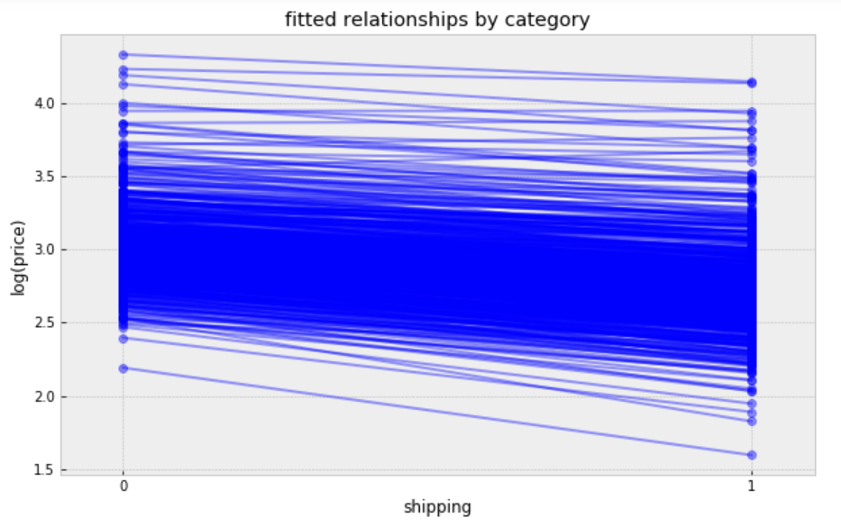
we wanted to make a prediction for a new product in “Women/Athletic Apparel/Pants, Tights, Leggings” category, which shipping paid by seller, we just need to sample from the model with the appropriate intercept.
The mean value sampled from this fit is ≈3, so we should expect the measured price in a new product in “Women/Athletic Apparel/Pants, Tights, Leggings” category, when shipping paid by seller, to be ≈exp(3) ≈ 20.09, though the range of predicted values is rather wide.
To give a bit of a background, I joined big N company for a bit over an year now for an ml research position, after finishing grad school and having some moderate success in academic research.
During my time here my team has been involved in 3 projects. And results have ranged from failure to success that hardly resulted from researching ml. time put into ml optimization resulting in only marginal improvements, and most actual value coming from unrelated stuff. Currently, even though our evaluations seem to be pretty good I think I am not bringing all that much value to the company. I really hope that I’ve had a rough start and it gets better, but wanted to hear others experiences.
We are creating a sparse training library for Pytorch. Sparse training is when only a fraction of the total parameters go through a forwards pass / backwards pass / update during each step.
Having all parameters takes up a lot of GPU memory, and in some cases may limit the total number of parameters your system can hold. By having the parameters stored on disk when not in use, that would significantly reduce the GPU memory used at any given instance, allowing you to use many more parameters.
A concern is that generally disk are not low enough latency to make this work. But we were able to figure out a pipeline to make it work. Not only that, but through a few Pytorch tricks we inadvertently discovered along the way, we think our set up may be (very slightly) faster, though we’ll need to do a bunch of test to absolutely confirm.
At the moment we need to code each adapt each architecture individually. If you or anyone you know have sparse training architecture you have in mind, point us to the paper or code and we’ll optimize and include it.
So far we’ve only been able to find recommender systems that make use of such architectures. If you know of any other architectures, please point them out.
ma-gym is a collection of simple multi-agent environments based on open ai gym with the intention of keeping the usage simple and exposing core challenges in multi-agent settings.
I made it during my recent internship and I hope it could be useful for others in their research or getting someone started with multi-agent reinforcement learning.
Implementations utilize deep reinforcement learning to train a policy neural network that parameterizes a policy for determining a robotic action based on a current state. Some of those implementations collect experience data from multiple robots that operate simultaneously. Each robot generates instances of experience data during iterative performance of episodes that are each explorations of performing a task, and that are each guided based on the policy network and the current policy parameters for the policy network during the episode. The collected experience data is generated during the episodes and is used to train the policy network by iteratively updating policy parameters of the policy network based on a batch of collected experience data. Further, prior to performance of each of a plurality of episodes performed by the robots, the current updated policy parameters can be provided (or retrieved) for utilization in performance of the episode.
That plot comes from a parameter search using Keras/Tensorflow for a binary classification problem with an unbalanced class distribution (as you can tell from the acc plot, the ratio is about 5:1 negative to positive).
The metric that I am most interested in is Precision, and as you can see in this example it is very unstable, bouncing around wildly between epochs – which obviously doesn’t lend itself to being a good/stable model.
Whilst there is a little overfitting, there doesn’t seem to be too much and I can confirm that the data itself is all properly scaled and normalised.
Although the plot scale is a bit large (sorry) to tell properly, I think what we’d find is that Recall fluctuates in unison with Precision. As Recall bounces upwards, I’d expect Precision to take a dive downwards.
I can’t post the exact model because it’s a parameter search with a wide range of possible configurations, but I’m optimising across a range of network depths, widths, dropouts, shapes, learning rate, etc. I’m using binary_crossentropy as the loss, Elu activations, and Nadam optimizer – though I’ve tried a various others with similar results.
What would be your suggestions for creating a more stable model?
At the moment, the class_weight is set to 0:1, 1:1. I think upping the positive class ratio would somewhat stabilise the model (by increasing recall), but I’m shooting to have a high precision and accepting that my recall will be the trade-off and be somewhat low. For example, I’d be happy with 57% precision at 5% recall. In fact – that’s the exact result I got from a previous parameter search, but it didn’t generalise well to the blind test set, and I’m suspecting that the cause was the unstable epoch-to-epoch precision we’re seeing in this plot (though I can only see the plots for the “current” model being generated, so by the end of the many-hour parameter search all I have is a csv of the final values, with no plots to go along with them).

