Creating a global footprint and access to scale are one of the many best practices at AWS. By creating architectures that take advantage of that scale and also efficient data utilization (in both performance and cost), you can start to see how important access is at scale. For example, within autonomous vehicles (AV) development, data is geographically acquired local to the driving campaign. It is relevant and more efficient from a machine learning (ML) perspective to execute the compute pipeline in the same AWS Region as the generated data.

To elaborate further, say that your organization acquires 4K video data on a driving campaign in San Francisco, United States. In parallel, your colleagues acquire a driving campaign in Stuttgart, Germany. Both video campaigns can result in a few TBs of data per day. Ideally, you would transfer the data into Regions close to where you generated the data (in this case, us-west-1 and eu-central-1). If the workflow labels this data, then running the distributed training local to their respective Regions makes sense from a cost and performance standpoint while maintaining consistency in the hyperparameters used to train both datasets.

To get started with distributed training on AWS, use Amazon SageMaker, which provisions much of the undifferentiated heavy lifting required for distributed training (for example, optimized TensorFlow with Horovod). Additionally, its per-second billing provides efficient cost management. These benefits free up your focus for model development and deployment in a fully managed architecture.

Amazon SageMaker is an ecosystem of managed ML services to help with ground truth labeling, model training, hyperparameter optimization, and deployment. You can access these services using Jupyter notebooks, the AWS CLI, or the Amazon SageMaker Python SDK. Particularly with the SDK, you need little code change to initiate and distribute the ML workload.

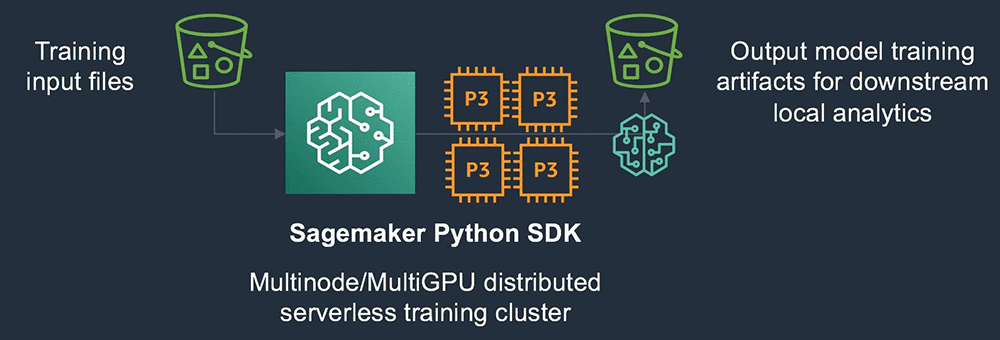
In the above architecture the S3 bucket serves as source for the training input files. The SageMaker Python SDK will instantiate the required compute resources and Docker image to run the model training sourcing the data from the S3. The output model artifacts are saved to an output S3 bucket.

Because the Amazon SageMaker Python SDK abstracts infrastructure deployment and is entirely API driven, you can orchestrate requests for training jobs via the SDK in scalable ways.

In the previous AV scenario, for example, you can trigger the input training data from the uploaded dataset, which you tracked in a relational way. You can couple this with AWS Batch, which offers a job array mechanism that can submit these distributed training jobs in a scalable way passing relevant hyperparameters at runtime. Consider the following example architecture.

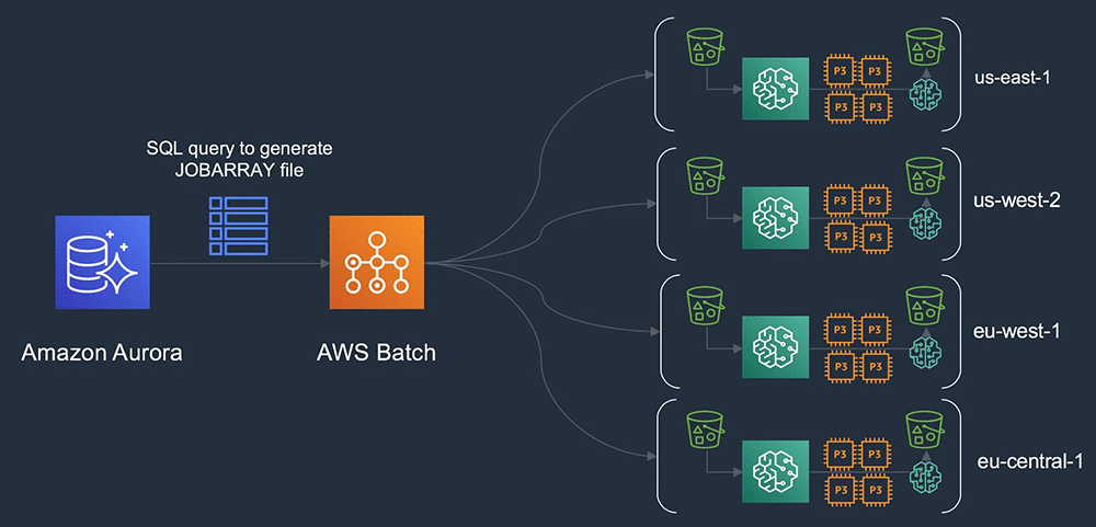
In this above architecture a relational database is used to track, for example, AV campaign metadata globally. A SQL query can be generated which populates the JOBARRAY input file in AWS Batch. AWS Batch then orchestrates the instantiation of the grid of clusters that are executed globally across multiple AWS Regions.

You are standing up a grid of clusters, globally deployed, based on data in Amazon S3 that is  generated locally. Querying the metadata from a central database to organize the training inputs with access to capacity across all four Regions. You can include some additional relational joins, which select data for transitive copy based on the On-Demand or Spot price per Region and reservation capacity.

Deploying Amazon SageMaker

The example in this post runs the Imagenet2012/Resnet50 model, with the Imagenet2012 TF records replicated across Regions. For this advanced workflow, you must prepare two Docker images. One image is for calling the Amazon SageMaker SDK to prepare the job submission, and the second image is for running the Horovod-enabled TensorFlow 1.13 environment.

First, create an IAM role to call the Amazon SageMaker service and subsequent services to run the training. Then, create the dl-sagemaker.py script. This is the main call script into the Amazon SageMaker training API.

For instructions on building the Amazon SageMaker Script Mode Docker image, see the TensorFlow framework repo on GitHub, in aws/sagemaker-tensorflow-container. After it’s built, commit this image to each Region in which you plan to generate data.

The following example commits this to us-east-1 (Northern Virginia), us-west-2 (Oregon), eu-west-1 (Ireland), and eu-central-1 (Frankfurt). When support for TensorFlow 1.13 with Tensorpack is in the Amazon SageMaker Python SDK, this becomes an optional step. To simplify the deployment, keep the name of the Amazon ECR image the same throughout Regions.

For the main entry script to call the Amazon SageMaker SDK (dl-sagemaker.py), complete the following steps:

1. Replace the entry:

   role = 'arn:aws:iam::<account-id>:role/sagemaker-sdk'

2. Replace the image_name with the name of the Docker image that you created:

   import os
   from sagemaker.session import s3_input
   from sagemaker.tensorflow import TensorFlow
   
   role = 'arn:aws:iam::<account-id>:role/sagemaker-sdk'
   
   num_gpus = int(os.environ.get('GPUS_PER_HOST'))
   
   distributions={
   'mpi': {
   'enabled': True,
   'processes_per_host': num_gpus,
   'custom_mpi_options': '-mca btl_vader_single_copy_mechanism none -x HOROVOD_HIERARCHICAL_ALLREDUCE=1 -x HOROVOD_FUSION_THRESHOLD=16777216 -x NCCL_MIN_NRINGS=8 -x NCCL_LAUNCH_MODE=PARALLEL'
   }
   }
   
   def main(aws_region,s3_location):
   estimator = TensorFlow(
   train_instance_type='ml.p3.16xlarge',
   train_volume_size=100,
   train_instance_count=10,
   framework_version='1.12',
   py_version='py3',
   image_name="<account id>.dkr.ecr.%s.amazonaws.com/sage-py3-tf-hvd:latest"%aws_region,
   entry_point='sagemaker_entry.py',
   dependencies=['/Users/amrraga/git/github/deep-learning-models'],
   script_mode=True,
   role=role,
   distributions=distributions,
   base_job_name='dist-test',
   )
   estimator.fit(s3_location)
   
   if __name__ == '__main__':
   aws_region = os.environ.get('AWS_DEFAULT_REGION')
   s3_location = os.environ.get('S3_LOCATION')
   
   main(aws_region,s3_location)

The following code is for sagemaker_entry.py, the inner call to initiate the training script:

import subprocess
import os

if __name__ =='__main__':
    train_dir = os.environ.get('SM_CHANNEL_TRAIN')
    subprocess.call(['python','-W ignore', 'deep-learning-models/models/resnet/tensorflow/train_imagenet_resnet_hvd.py', 
            "—data_dir=%s"%train_dir, 
            '—num_epochs=90', 
            '-b=256', 
            '—lr_decay_mode=poly', 
            '—warmup_epochs=10', 
            '—clear_log'])

The following code is for sage_wrapper.sh, the overall wrapper for AWS Batch to download the array definition from S3 and initiate the global Amazon SageMaker API calls:

#!/bin/bash -xe
###################################
env
###################################
echo "DOWNLOADING SAGEMAKER MANIFEST ARRAY FILES..."
aws s3 cp $S3_ARRAY_FILE sage_array.txt
if [[ -z "${AWS_BATCH_JOB_ARRAY_INDEX}" ]]; then
   echo "NOT AN ARRAY JOB...EXITING"
   exit 1
else
   LINE=$((AWS_BATCH_JOB_ARRAY_INDEX + 1))
   SAGE_SYSTEM=$(sed -n ${LINE}p sage_array.txt)
   while IFS=, read -r f1 f2 f3; do
           export AWS_DEFAULT_REGION=${f1}
           export S3_LOCATION=${f2}
   done <<< $SAGE_SYSTEM
fi

GPUS_PER_HOST=8 python3 dl-sagemaker.py

echo "SAGEMAKER TRAINING COMPLETE"
exit 0

Lastly, the following code is for the Dockerfile, to build the batch orchestration image:

FROM amazonlinux:latest

### SAGEMAKER PYTHON SDK

RUN yum update -y
RUN amazon-linux-extras install epel
RUN yum install python3-pip git -y
RUN pip3 install tensorflow sagemaker awscli

### API SCRIPTS

RUN mkdir /api
ADD dl-sagemaker.py /api
ADD sagemaker_entry.py /api
ADD sage_wrapper.sh /api
RUN chmod +x /api/sage_wrapper.sh

### SAGEMAKER SDK DEPENDENCIES

RUN git clone https://github.com/aws-samples/deep-learning-models.git /api/deep-learning-models

Commit the built Docker image to ECR in the same Region as the Amazon SageMaker Python SDK. From this Region, you can deploy all your Amazon SageMaker distributed ML cluster-workers globally.

With AWS Batch, you don’t need any unique configurations to instantiate a compute environment. Because you are just using AWS Batch to launch the Amazon SageMaker APIs, the default settings are enough. Attach a job queue to the compute environment and create the job definition file with the following:

{
    "jobDefinitionName": "sagemaker-python-sdk-jobdef",
    "jobDefinitionArn": "arn:aws:batch:us-east-1:<accountid>:job-definition/sagemaker-python-sdk-jobdef:1",
    "revision": 1,
    "status": "ACTIVE",
    "type": "container",
    "parameters": {},
    "containerProperties": {
        "image": "<accountid>.dkr.ecr.us-east-1.amazonaws.com/batch/sagemaker-sdk:latest",
        "vcpus": 2,
        "memory": 2048,
        "command": [
            "/api/sage_wrapper.sh"
        ],
        "jobRoleArn": "arn:aws:iam::<accountid>:role/ecsTaskExecutionRole",
        "volumes": [],
        "environment": [
            {
                "name": "S3_ARRAY_FILE",
                "value": "s3://ragab-ml/"
            }
        ],
        "mountPoints": [],
        "ulimits": [],
        "resourceRequirements": []
    }
}

To import at job startup, upload an example JOBARRAY file to S3:

us-east-1,s3://ragab-ml/imagenet2012/tf-imagenet/resized
us-west-2,s3://ragab-ml-pdx/imagenet2012/tf-imagenet/resized
eu-west-1,s3://ragab-ml-dub/imagenet2012/tf-imagenet/resized
eu-central-1,s3://ragab-ml-fra/imagenet2012/tf-imagenet/resized

On the Jobs page, submit a job that changes the path of the S3_ARRAY_FILE. A job array starts up with each node dedicated to submitting and monitoring an ML training job in a separate Region. If you select a candidate Region where a job is running, you can see additional algorithms, instance metrics, and further log details.

One notable aspect of this deployment is that in the previous example, you launched a grid of clusters of 480 GPUs over four Regions, totaling 360,000 images/sec combined. This process improved time to results and optimized parameter scanning.

Conclusion

By implementing this architecture, you now have a scalable, performant, globally distributed ML training platform. In the AWS Batch script, you can lift any number of parameters into the array file to distribute the workload. For example, you can use not only different input training files, but also different hyperparameters, Docker container images, or even different algorithms, all deployed on a global scale.

Consider also that any backend, serverless distributed ML service can execute these workloads. For example, it is possible to replace the Amazon SageMaker components with Amazon EKS. Now go power up your ML workloads with a global footprint!

Open the Amazon SageMaker console to get started. If you have any questions, please leave them in the comments.

About the Author

Amr Ragab is a Business Development Manager in Accelerated Computing for AWS, devoted to helping customers run computational workloads at scale. In his spare time he likes traveling and finds ways to integrate technology into daily life.

Optimization is the process of finding the minimum (or maximum) of a function that depends on some inputs, called design variables. Customer X has the following problem: They are about to release a new car model to be designed for maximum fuel efficiency. In reality, thousands of parameters that represent tuning parameters relating to the engine, transmission, suspension, and so on. The combinations result in varying fuel efficiency values.

However, for this post, assume that they want to measure this efficiency as the gallons of fuel burned per hour when traveling at a particular speed, all other parameters being constant. Therefore, the “function” to be minimized is “gallons of fuel burned per hour” and the design variable is “speed.” This one-dimensional optimization problem asks the question: “What speed should the car be driven at for burning the minimum amount of fuel per hour,” which is a greatly simplified version of the thousands of actual parameters to be considered.

Assume that the objective function (f) looks like the following synthetic function:

f(x) = x⋅sin(x)+x⋅cos(2x)

Ignoring the units on the x and y axes, your task is to find the minimum of this function, indicated by the blue arrow. Even when dealing with a single dimension, it is impractical to run the car over every speed value (speed being a real number).

For this post, you have a budget of running 30 experiments, each “experiment” consisting of running the car on a test rig at that speed, measuring and collecting the average value of fuel burned per hour. This gives you 30 values of fuel burned, corresponding to 30 values of speeds, and nothing more. There is also no guarantee that there was an experiment conducted at the value of speed indicated by the minimum (blue arrow in the figure).

Each experiment can actually take hours to set up. Because it is impractical to do more than a certain number of such experiments, this type of function is called an expensive, black-box function. It’s expensive because the function takes time to return a value, and black-box as the experiments conducted can’t be written as mathematical expressions.

The entire field of optimization research is targeted towards creating algorithms to solve these kinds of problems. In this post, you use a neural network to approximate the function (f) above. This trained approximation of the function, also known as a “surrogate model,” can be used instead of actual experiments! If the trained model is a good approximation of the actual function, the model can be used to predict the fuel burned (output) for any value of speed (input).

Technical approach

For a sample Jupyter notebook that walks through all these steps, see Build a Deep Neural Global Optimizer.

Given the function (f), measure the value of the output given the values of various inputs. You create a simple, four-layer network, based on the recommendations in Scalable Bayesian Optimization Using Deep Neural Networks:

1. Input layer (tanh activation)
2. Hidden layer 1 (tanh activation)
3. Hidden layer 2 (tanh activation)
4. Output layer (ReLU activation)

In PyTorch, this can be written as follows:

def __init__(self, D_in, H, D, D_out):
    """
    In the constructor, instantiate two nn.Linear modules and assign them as
    member variables.
    """
    super(Net, self).__init__()
    self.inputlayer = nn.Linear(D_in, H)
    self.middle = nn.Linear(H, H)
    self.lasthiddenlayer = nn.Linear(H, D)
    self.outputlayer = nn.Linear(D, D_out)

Where D_in, H, D and D_out are used to define the parameter matrix sizes within the function.

You are also required to specify the activation function for each neuron, and how inputs are transformed in the forward pass:

def forward(self, x):
    """
    In the forward function, accept a variable of input data and return
    a variable of output data. Use modules defined in the constructor, as
    well as arbitrary operators on variables.
    """
    y_pred = self.outputlayer(self.PHI(x))
    return y_pred
    
def PHI(self, x):
    h_relu = self.inputlayer(x).tanh()
    for i in range(2):
        h_relu = self.middle(h_relu).tanh()
    phi = self.lasthiddenlayer(h_relu)
    return phi

In the train function, use Mean Squared Error as the loss function and use the Adam optimizer:

self.network = Net(features, self.H, self.D, 1) # here we suppose that D_out = 1
loss_fn = torch.nn.MSELoss(size_average=True)
optimizer = torch.optim.Adam(self.network.parameters(), lr=self.init_learning_rate)

To collect data from the experiments, sample the function f(x) = x⋅sin(x)+x⋅cos(2x) at random points. In the figure below, the black dashed line represents all values of f(x) in that range of x (here, 0 to 10), and the red dots represent the 30 sampled points.

To reiterate, the goal of the network is to use the training data (x and y axis values corresponding to the sampled data points) to learn to approximate the function. Provided that the neural network has learned a good approximation of the original function f(x), you can use the trained model to predict the values of the outputs, given inputs, without running an expensive or a time-consuming experiment.

If you’re interested in the more technical details, see Scalable Bayesian Optimization Using Deep Neural Networks. In brief, a Bayesian linear regressor is added to the last hidden layer of a deep neural network. This results in adaptive basis regression, a well-established statistical technique that scales linearly in the number of observations. These “basis functions” are parameterized using the weights and biases of the deep neural network. Finally, the mean and variance of the prediction can then be calculated using the formulae (4) and (5) in the Scalable Bayesian Optimization paper. So, you are not only obtaining a function approximation, but also the uncertainty associated with the predicted points.

Given the small size of the input vector, you train the model on a notebook instance with the conda36_pytorch kernel. I highly encourage you to resort to distributed training using Amazon SageMaker rather than local training when appropriate. The following command starts the training process:

deepgaussian.train(DOE,yvalues)

In PyTorch, the training loop is implemented as follows:

for t in range(self.num_epochs):
    y_pred = self.network(self.X)
    loss = loss_fn(y_pred.view(-1), self.Y.view(-1))
    optimizer.zero_grad()
    loss.backward()
    optimizer.step()

Obtain the following output indicating that the network has been trained:

Optimization terminated successfully.
         Current function value: 6.652170
         Iterations: 49
         Function evaluations: 99

Finally, plot the surrogate model using a set of test values (xtest), as follows:

mean, var = deepgaussian.predict(x_test)
plt.figure(figsize=(20,10))
plt.rcParams.update({'font.size': 22})
plt.plot(DOE, yvalues, "ro",label='Sampled Points',markersize=10)
plt.plot(xtest[:,0], fvals, "k--", label = 'Actual function')
plt.plot(xtest[:,0], mean, "blue",label='Surrogate function')
plt.fill_between(xtest[:, 0], mean + np.sqrt(var), mean - np.sqrt(var), color="orange", alpha=0.4, label='+/- Variance')
plt.grid()
plt.legend()
plt.show()

You obtain the following image:

As you can see, the network has learned the shape of the function f(x) accurately, and also associates some uncertainty with each point it used for prediction. Here, the blue lines are prediction means and the orange band is the uncertainty associated with each of the predictions.

Conclusion

At this point, the model can be used to predict any number of experimental output values within a confidence interval, without actually performing the experiment. What is more useful is using an optimization package to find the optimum input value that corresponds to the minimum f(x) value. To start, see the scipy.optimize or inspyred packages.

Lastly, this is a starter example that runs locally on a notebook instance. Get started now by launching the Amazon SageMaker console and exploring distributed training on Amazon Sagemaker. For large-scale optimization jobs, consider doing distributed training on Amazon SageMaker by submitting the PyTorch script to the Amazon SageMaker Pytorch estimator.

About the Author

Shreyas Subramanian is a AI/ML specialist Solutions Architect, and helps customers by using Machine Learning to solve their business challenges using the AWS platform.