Posted by Joonseok Lee and Joe Yue-Hei Ng, Software Engineers, Google Research

Over the last two years, the First and Second YouTube-8M Large-Scale Video Understanding Challenge and Workshop have collectively drawn 1000+ teams from 60+ countries to further advance large-scale video understanding research. While these events have enabled great progress in video classification, the YouTube dataset on which they were based only used machine-generated video-level labels, and lacked fine-grained temporally localized information, which limited the ability of machine learning models to predict video content.

To accelerate the research of temporal concept localization, we are excited to announce the release of YouTube-8M Segments, a new extension of the YouTube-8M dataset that includes human-verified labels at the 5-second segment level on a subset of YouTube-8M videos. With the additional temporal annotations, YouTube-8M is now both a large-scale classification dataset as well as a temporal localization dataset. In addition, we are hosting another Kaggle video understanding challenge focused on temporal localization, as well as an affiliated 3rd Workshop on YouTube-8M Large-Scale Video Understanding at the 2019 International Conference on Computer Vision (ICCV’19).

YouTube-8M Segments
Video segment labels provide a valuable resource for temporal localization not possible with video-level labels, and enable novel applications, such as capturing special video moments. Instead of exhaustively labeling all segments in a video, to create the YouTube-8M Segments extension, we manually labeled 5 segments (on average) per randomly selected video on the YouTube-8M validation dataset, totalling ~237k segments covering 1000 categories.

This dataset, combined with the previous YouTube-8M release containing a very large number of machine generated video-level labels, should allow learning temporal localization models in novel ways. Evaluating such classifiers is of course very challenging if only noisy video-level labels are available. We hope that the newly added human-labeled annotations will help ensure that researchers can more accurately evaluate their algorithms.

The 3rd YouTube-8M Video Understanding Challenge
This year the YouTube-8M Video Understanding Challenge focuses on temporal localization. Participants are encouraged to leverage noisy video-level labels together with a small segment-level validation set in order to better annotate and temporally localize concepts of interest. Unlike last year, there is no model size restriction. Each of the top 10 teams will be awarded $2,500 to support their travel to Seoul to attend ICCV’19. For details, please visit the Kaggle competition page.

The 3rd Workshop on YouTube-8M Large-Scale Video Understanding
Continuing in the tradition of the previous two years, the 3rd workshop will feature four invited talks by distinguished researchers as well as presentations by top-performing challenge participants. We encourage those who wish to attend to submit papers describing their research, experiments, or applications based on the YouTube-8M dataset, including papers summarizing their participation in the challenge above. Please refer to the workshop page for more details.

It is our hope that this newest extension will serve as a unique playground for temporal localization that mimics real world scenarios. We also look forward to the new challenge and workshop, which we believe will continue to advance research in large-scale video understanding. We hope you will join us again!

Acknowledgements
This post reflects the work of many machine perception researchers including Ke Chen, Nisarg Kothari, Joonseok Lee, Hanhan Li, Paul Natsev, Joe Yue-Hei Ng, Naderi Parizi, David Ross, Cordelia Schmid, Javier Snaider, Rahul Sukthankar, George Toderici, Balakrishnan Varadarajan, Sudheendra Vijayanarasimhan, Yexin Wang, Zheng Xu, as well as Julia Elliott and Walter Reade from Kaggle. We are also grateful for the support and advice from our partners at YouTube.

Posted by Alex Fabrikant, Research Scientist, Google Research

Hundreds of millions of people across the world rely on public transit for their daily commute, and over half of the world’s transit trips involve buses. As the world’s cities continue growing, commuters want to know when to expect delays, especially for bus rides, which are prone to getting held up by traffic. While public transit directions provided by Google Maps are informed by many transit agencies that provide real-time data, there are many agencies that can’t provide them due to technical and resource constraints.

Today, Google Maps introduced live traffic delays for buses, forecasting bus delays in hundreds of cities world-wide, ranging from Atlanta to Zagreb to Istanbul to Manila and more. This improves the accuracy of transit timing for over sixty million people. This system, first launched in India three weeks ago, is driven by a machine learning model that combines real-time car traffic forecasts with data on bus routes and stops to better predict how long a bus trip will take.

The Beginnings of a Model
In the many cities without real-time forecasts from the transit agency, we heard from surveyed users that they employed a clever workaround to roughly estimate bus delays: using Google Maps driving directions. But buses are not just large cars. They stop at bus stops; take longer to accelerate, slow down, and turn; and sometimes even have special road privileges, like bus-only lanes.

As an example, let’s examine a Wednesday afternoon bus ride in Sydney. The actual motion of the bus (blue) is running a few minutes behind the published schedule (black). Car traffic speeds (red) do affect the bus, such as the slowdown at 2000 meters, but a long stop at the 800 meter mark slows the bus down significantly compared to a car.

To develop our model, we extracted training data from sequences of bus positions over time, as received from transit agencies’ real time feeds, and aligned them to car traffic speeds on the bus’s path during the trip. The model is split into a sequence of timeline units—visits to street blocks and stops—each corresponding to a piece of the bus’s timeline, with each unit forecasting a duration. A pair of adjacent observations usually spans many units, due to infrequent reporting, fast-moving buses, and short blocks and stops.

This structure is well suited for neural sequence models like those that have recently been successfully applied to speech processing, machine translation, etc. Our model is simpler. Each unit predicts its duration independently, and the final output is the sum of the per-unit forecasts. Unlike many sequence models, our model does not need to learn to combine unit outputs, nor to pass state through the unit sequence. Instead, the sequence structure lets us jointly (1) train models of individual units’ durations and (2) optimize the “linear system” where each observed trajectory assigns a total duration to the sum of the many units it spans.

To model a bus trip (a) starting at the blue stop, the model (b) adds up the delay predictions from timeline units for the blue stop, the three road segments, the white stop, etc.

Modeling the “Where”
In addition to road traffic delays, in training our model we also take into account details about the bus route, as well as signals about the trip’s location and timing. Even within a small neighborhood, the model needs to translate car speed predictions into bus speeds differently on different streets. In the left panel below, we color-code our model’s predicted ratio between car speeds and bus speeds for a bus trip. Redder, slower parts may correspond to bus deceleration near stops. As for the fast green stretch in the highlighted box, we learn from looking at it in StreetView (right) that our model discovered a bus-only turn lane. By the way, this route is in Australia, where right turns are slower than left, another aspect that would be lost on a model that doesn’t consider peculiarities of location.

To capture unique properties of specific streets, neighborhoods, and cities, we let the model learn a hierarchy of representations for areas of different size, with a timeline unit’s geography (the precise location of a road or a stop) represented in the model by the sum of the embeddings of its location at various scales. We first train the model with progressively heavier penalties for finer-grain locations with special cases, and use the results for feature selection. This ensures that fine-grained features in areas complex enough where a hundred meters affects bus behavior are taken into account, as opposed to open countryside where such fine-grained features seldom matter.

At training time, we also simulate the possibility of later queries about areas that were not in the training data. In each training batch, we take a random slice of examples and discard geographic features below a scale randomly selected for each. Some examples are kept with the exact bus route and street, others keep only neighborhood- or city-level locations, and others yet have no geographical context at all. This better prepares the model for later queries about areas where we were short on training data. We expand the coverage of our training corpus by using anonymized inferences about user bus trips from the same dataset that Google Maps uses for popular times at businesses, parking difficulty, and other features. However, even this data does not include the majority of the world’s bus routes, so our models must generalize robustly to new areas.

Learning the Local Rhythms
Different cities and neighborhoods also run to a different beat, so we allow the model to combine its representation of location with time signals. Buses have a complex dependence on time — the difference between 6:30pm and 6:45pm on a Tuesday might be the wind-down of rush hour in some neighborhoods, a busy dining time in others, and entirely quiet in a sleepy town elsewhere. Our model learns an embedding of the local time of day and day of week signals, which, when combined with the location representation, captures salient local variations, like rush hour bus stop crowds, that aren’t observed via car traffic.

This embedding assigns 4-dimensional vectors to times of the day. Unlike most neural net internals, four dimensions is almost few enough to visualize, so let’s peek at how the model arranges times of day in three of those dimensions, via the artistic rendering below. The model indeed learns that time is cyclical, placing time in a “loop”. But this loop is not just the flat circle of a clock’s face. The model learns wide bends that let other neurons compose simple rules to easily separate away concepts like “middle of the night” or “late morning” that don’t feature much bus behavior variation. On the other hand, evening commute patterns differ much more among neighborhoods and cities, and the model appears to create more complex “crumpled” patterns between 4pm-9pm that enable more intricate inferences about the timings of each city’s rush hour.

The model’s time representation (3 out of 4 dimensions) forms a loop, reimagined here as the circumference of a watch. The more location-dependent time windows like 4pm-9pm and 7am-9am get more complex “crumpling”, while big featureless windows like 2am-5am get bent away with flat bends for simpler rules. (Artist’s conception by Will Cassella, using textures from textures.com and HDRIs from hdrihaven.)

Together with other signals, this time representation lets us predict complex patterns even if we hold car speeds constant. On a 10km bus ride through New Jersey, for example, our model picks up on lunchtime crowds and weekday rush hours:

Putting it All Together
With the model fully trained, let’s take a look at what it learned about the Sydney bus ride above. If we run the model on that day’s car traffic data, it gives us the green predictions below. It doesn’t catch everything. For instance, it has the stop at 800 meters lasting only 10 seconds, though the bus stopped for at least 31 sec. But we stay within 1.5 minutes of the real bus motion, catching a lot more of the trip’s nuances than the schedule or car driving times alone would give us.

The Trip Ahead
One thing not in our model for now? The bus schedule itself. So far, in experiments with official agency bus schedules, they haven’t improved our forecasts significantly. In some cities, severe traffic fluctuations might overwhelm attempts to plan a schedule. In others, the bus schedules might be precise, but perhaps because transit agencies carefully account for traffic patterns. And we infer those from the data.

We continue to experiment with making better use of schedule constraints and many other signals to drive more precise forecasting and make it easier for our users to plan their trips. We hope we’ll be of use to you on your way, too. Happy travels!

Acknowledgements
This work was the joint effort of James Cook, Alex Fabrikant, Ivan Kuznetsov, and Fangzhou Xu, on Google Research, and Anthony Bertuca, Julian Gibbons, Thierry Le Boulengé, Cayden Meyer, Anatoli Plotnikov, and Ivan Volosyuk on Google Maps. We thank Senaka Buthpitiya, Da-Cheng Juan, Reuben Kan, Ramesh Nagarajan, Andrew Tomkins, and the greater Transit team for support and helpful discussions; as well as Will Cassella for the inspired reimagining of the model’s time embedding. We are also indebted to our partner agencies for providing the transit data feeds the system is trained on.

Posted by Alessandro Epasto, Senior Research Scientist and Bryan Perozzi, Senior Research Scientist, Graph Mining Team

Relational data representing relationships between entities is ubiquitous on the Web (e.g., online social networks) and in the physical world (e.g., in protein interaction networks). Such data can be represented as a graph with nodes (e.g., users, proteins), and edges connecting them (e.g., friendship relations, protein interactions). Given the widespread prevalence of graphs, graph analysis plays a fundamental role in machine learning, with applications in clustering, link prediction, privacy, and others. To apply machine learning methods to graphs (e.g., predicting new friendships, or discovering unknown protein interactions) one needs to learn a representation of the graph that is amenable to be used in ML algorithms.

However, graphs are inherently combinatorial structures made of discrete parts like nodes and edges, while many common ML methods, like neural networks, favor continuous structures, in particular vector representations. Vector representations are particularly important in neural networks, as they can be directly used as input layers. To get around the difficulties in using discrete graph representations in ML, graph embedding methods learn a continuous vector space for the graph, assigning each node (and/or edge) in the graph to a specific position in a vector space. A popular approach in this area is that of random-walk-based representation learning, as introduced in DeepWalk.

Left: The well-known Karate graph representing a social network. Right: A continuous space embedding of the nodes in the graph using DeepWalk.

Here we present the results of two recent papers on graph embedding: “Is a Single Embedding Enough? Learning Node Representations that Capture Multiple Social Contexts” presented at WWW’19 and “Watch Your Step: Learning Node Embeddings via Graph Attention” at NeurIPS’18. The first paper introduces a novel technique to learn multiple embeddings per node, enabling a better characterization of networks with overlapping communities. The second addresses the fundamental problem of hyperparameter tuning in graph embeddings, allowing one to easily deploy graph embeddings methods with less effort. We are also happy to announce that we have released the code for both papers in the Google Research github repository for graph embeddings.

Learning Node Representations that Capture Multiple Social Contexts
In virtually all cases, the crucial assumption of standard graph embedding methods is that a single embedding has to be learned for each node. Thus, the embedding method can be said to seek to identify the single role or position that characterizes each node in the geometry of the graph. Recent work observed, however, that nodes in real networks belong to multiple overlapping communities and play multiple roles—think about your social network where you participate in both your family and in your work community. This observation motivates the following research question: is it possible to develop methods where nodes are embedded in multiple vectors, representing their participation in overlapping communities?

In our WWW’19 paper, we developed Splitter, an unsupervised embedding method that allows the nodes in a graph to have multiple embeddings to better encode their participation in multiple communities. Our method is based on recent innovations in overlapping clustering based on ego-network analysis, using the persona graph concept, in particular. This method takes a graph G, and creates a new graph P (called the persona graph), where each node in G is represented by a series of replicas called the persona nodes. Each persona of a node represents an instantiation of the node in a local community to which it belongs. For each node U in the graph, we analyze the ego-network of the node (i.e., the graph connecting the node to its neighbors, in this example A, B, C, D) to discover local communities to which the node belongs. For instance, in the figure below, node U belongs to two communities: Cluster 1 (with the friends A and B, say U’s family members) and Cluster 2 (with C and D, say U’s colleagues).

Ego-net of node U

Then, we use this information to “split” node U into its two personas U1 (the family persona) and U2 (the work persona). This disentangles the two communities, so that they no longer overlap.

The ego-splitting method separating the U nodes in 2 personas.

This technique has been used to improve the state-of-the-art results in graph embedding methods, showing up to 90% reduction in link prediction (i.e., predicting which link will form in the future) error on a variety of graphs. The key reason for this improvement is the ability of the method to disambiguate highly overlapping communities found in social networks and other real-world graphs. We further validate this result with an in-depth analysis of co-authorship graphs where authors belong to overlapping research communities (e.g., machine learning and data mining).

Top Left: A typical graphs with highly overlapping communities. Top Right: A traditional embedding of the graph on the left using node2vec. Bottom Left: A persona graph of the graph above. Bottom Right: The Splitter embedding of the persona graph. Notice how the persona graph clearly disentangles the overlapping communities of the original graph and Splitter outputs well-separated embeddings.

Automatic hyper-parameter tuning via graph attention.
Graph embedding methods have shown outstanding performance on various ML-based applications, such as link prediction and node classification, but they have a number of hyper-parameters that must be manually set. For example, are nearby nodes more important to capture when learning embeddings than nodes that are further away? Even though experts may be able to fine tune these hyper-parameters, one must do so independently for each graph. To obviate such manual work, in our second paper, we proposed a method to learn the optimal hyper-parameters automatically.

Specifically, many graph embedding methods, like DeepWalk, employ random walks to explore the context around a given node (i.e. the direct neighbors, the neighbors of the neighbors, etc). Such random walks can have many hyper-parameters that allow tuning of the local exploration of the graph, thus regulating the attention given by the embeddings to nearby nodes. Different graphs may present different optimal attention patterns and hence different optimal hyperparameters (see the picture below, where we show two different attention distributions). Watch Your Step formulates a model for the performance of the embedding methods based on the above mentioned hyper-parameters. Then we optimize the hyper-parameters to maximize the performance predicted by the model, using standard backpropagation. We found that the values learned by backpropagation agree with the optimal hyper-parameters obtained by grid search.

Our new method for automatic hyper-parameter tuning, Watch Your Step, uses an attention model to learn different graph context distributions. Shown above are two example local neighborhoods about a center node (in yellow) and the context distributions (red gradient) that was learned by the model. The left-side graph shows a more diffused attention model, while the distribution on the right shows one concentrated on direct neighbors.

This work falls under the growing family of AutoML, where we want to alleviate the burden of optimizing the hyperparameters—a common problem in practical machine learning. Many AutoML methods use neural architecture search. This paper instead shows a variant, where we use the mathematical connection between the hyperparameters in the embeddings and graph-theoretic matrix formulations. The “Auto” portion corresponds to learning the graph hyperparameters by backpropagation.

We believe that our contributions will further advance the state of the research in graph embedding in various directions. Our method for learning multiple node embeddings draws a connection between the rich and well-studied field of overlapping community detection, and the more recent one of graph embedding which we believe may result in fruitful future research. An open problem in this area is the use of multiple-embedding methods for classification. Furthermore, our contribution on learning hyperparameters will foster graph embedding adoption by reducing the need for expensive manual tuning. We hope the release of these papers and code will help the research community pursue these directions.

Acknowledgements
We thank Sami Abu-el-Haija who contributed to this work and is now a Ph.D. student at USC.

Posted by Alex Irpan, Software Engineer, Robotics at Google

Reinforcement learning (RL) is a framework that lets agents learn decision making from experience. One of the many variants of RL is off-policy RL, where an agent is trained using a combination of data collected by other agents (off-policy data) and data it collects itself to learn generalizable skills like robotic walking and grasping. In contrast, fully off-policy RL is a variant in which an agent learns entirely from older data, which is appealing because it enables model iteration without requiring a physical robot. With fully off-policy RL, one can train several models on the same fixed dataset collected by previous agents, then select the best one. However, fully off-policy RL comes with a catch: while training can occur without a real robot, evaluation of the models cannot. Furthermore, ground-truth evaluation with a physical robot is too inefficient to test promising approaches that require evaluating a large number of models, such as automated architecture search with AutoML.

This challenge motivates off-policy evaluation (OPE), techniques for studying the quality of new agents using data from other agents. With rankings from OPE, we can selectively test only the most promising models on real-world robots, significantly scaling experimentation with the same fixed real robot budget.

A diagram for real-world model development. Assuming we can evaluate 10 models per day, without off-policy evaluation, we would need 100x as many days to evaluate our models.

Though the OPE framework shows promise, it assumes one has an off-policy evaluation method that accurately ranks performance from old data. However, agents that collected past experience may act very differently from newer learned agents, which makes it hard to get good estimates of performance.

In “Off-Policy Evaluation via Off-Policy Classification”, we propose a new off-policy evaluation method, called off-policy classification (OPC), that evaluates the performance of agents from past data by treating evaluation as a classification problem, in which actions are labeled as either potentially leading to success or guaranteed to result in failure. Our method works for image (camera) inputs, and doesn’t require reweighting data with importance sampling or using accurate models of the target environment, two approaches commonly used in prior work. We show that OPC scales to larger tasks, including a vision-based robotic grasping task in the real world.

How OPC Works
OPC relies on two assumptions: 1) that the final task has deterministic dynamics, i.e. no randomness is involved in how states change, and 2) that the agent either succeeds or fails at the end of each trial. This second “success or failure” assumption is natural for many tasks, such as picking up an object, solving a maze, winning a game, and so on. Because each trial will either succeed or fail in a deterministic way, we can assign binary classification labels to each action. We say an action is effective if it could lead to success, and is catastrophic if it is guaranteed to lead to failure.

OPC utilizes a Q-function, learned with a Q-learning algorithm, that estimates the future total reward if the agent chooses to take some action from its current state. The agent will then choose the action with the largest total reward estimate. In our paper, we prove that the performance of an agent is measured by how often its chosen action is an effective action, which depends on how well the Q-function correctly classifies actions as effective vs. catastrophic. This classification accuracy acts as an off-policy evaluation score.

However, the labeling of data from previous trials is only partial. For example, if a previous trial was a failure, we do not get negative labels because we do not know which action was the catastrophic one. To overcome this, we leverage techniques from semi-supervised learning, positive-unlabeled learning in particular, to get an estimate of classification accuracy from partially labeled data. This accuracy is the OPC score.

Off-Policy Evaluation for Sim-to-Real Learning
In robotics, it’s common to use simulated data and transfer learning techniques to reduce the sample complexity of learning robotics skills. This can be very useful, but tuning these sim-to-real techniques for real-world robotics is challenging. Much like off-policy RL, training doesn’t use the real robot, because it is trained in simulation, but evaluation of that policy still needs to use a real robot. Here, off-policy evaluation can come to the rescue again—we can take a policy trained only in simulation, then evaluate it using previous real-world data to measure its transfer to the real robot. We examine OPC across both fully off-policy RL and sim-to-real RL.

An example of how simulated experience can differ from real-world experience. Here, simulated images (left) have much less visual complexity than real-world images (right).

Results
First, we set up a simulated version of our robot grasping task, where we could easily train and evaluate several models to benchmark off-policy evaluation. These models were trained with fully off-policy RL, then evaluated with off-policy evaluation. We found that in our robotics tasks, a variant of the OPC called the SoftOPC performed best at predicting final success rate.

An experiment in the simulated grasping task. The red curve is the dimensionless SoftOPC score over the course of training, evaluated from old data. The blue curve is the grasp success rate in simulation. We see the SoftOPC on old data correlates well with grasp success of the model within our simulator.

After success in sim, we then tried SoftOPC in the real-world task. We took 15 models, trained to have varying degrees of robustness to the gap between simulation and reality. Of these models, 7 of them were trained purely in simulation, and the rest were trained on mixes of simulated and real-world data. For each model, we evaluated the SoftOPC on off-policy real-world data, then the real-world grasp success, to see how well SoftOPC predicted performance of that model. We found that on real data, the SoftOPC does produce scores that correlate with true grasp success, letting us rank sim-to-real techniques using past real experience.

SoftOPC score and true performance for 3 different sim-to-real methods: a baseline simulation, a simulation with random textures and lighting, and a model trained with RCAN. All three models are trained with no real data, then evaluated with off-policy evaluation on a validation set of real data. The ordering of the SoftOPC score matches the order of real grasp success.

Below is a scatterplot of the full results from all 15 models. Each point represents the off-policy evaluation score and real-world grasp success of each model. We compare different scoring functions by their correlation to final grasp success. The SoftOPC does not correlate perfectly with true grasp success, but its scores are significantly more reliable than baseline approaches like the temporal-difference error (the standard Q-learning loss).

Results from our sim-to-real evaluation experiment. On the left is a baseline, the temporal difference error of the model. On the right is one of our proposed methods, the SoftOPC. The shaded region is a 95% confidence interval. The correlation is significantly better with SoftOPC.

Future Work
One promising direction for future work is to see if we can relax our assumptions about the task, to support tasks where dynamics are more noisy, or where we get partial credit for almost succeeding. However, even with our included assumptions, we think the results are promising enough to be applied to many real-world RL problems.

Acknowledgements
This research was conducted by Alex Irpan, Kanishka Rao, Konstantinos Bousmalis, Chris Harris, Julian Ibarz and Sergey Levine. We’d like to thank Razvan Pascanu, Dale Schuurmans, George Tucker and Paul Wohlhart for valuable discussions. A preprint is available on arXiv.

Posted by Andrew Helton, Editor, Google AI Communications

This week, Long Beach, CA hosts the 2019 Conference on Computer Vision and Pattern Recognition (CVPR 2019), the premier annual computer vision event comprising the main conference and several co-located workshops and tutorials. As a leader in computer vision research and a Platinum Sponsor, Google will have a strong presence at CVPR 2019—over 250 Googlers will be in attendance to present papers and invited talks at the conference, and to organize and participate in multiple workshops.

If you are attending CVPR this year, please stop by our booth and chat with our researchers who are actively pursuing the next generation of intelligent systems that utilize the latest machine learning techniques applied to various areas of machine perception. Our researchers will also be available to talk about and demo several recent efforts, including the technology behind predicting pedestrian motion, the Open Images V5 dataset and much more.

You can learn more about our research being presented at CVPR 2019 in the list below (Google affiliations highlighted in blue)

Area Chairs include:
Jonathan T. Barron, William T. Freeman, Ce Liu, Michael Ryoo, Noah Snavely

Oral Presentations
Relational Action Forecasting
Chen Sun, Abhinav Shrivastava, Carl Vondrick, Rahul Sukthankar, Kevin Murphy, Cordelia Schmid

Pushing the Boundaries of View Extrapolation With Multiplane Images
Pratul P. Srinivasan, Richard Tucker, Jonathan T. Barron, Ravi Ramamoorthi, Ren Ng, Noah Snavely

Auto-DeepLab: Hierarchical Neural Architecture Search for Semantic Image Segmentation
Chenxi Liu, Liang-Chieh Chen, Florian Schroff, Hartwig Adam, Wei Hua, Alan L. Yuille, Li Fei-Fei

AutoAugment: Learning Augmentation Strategies From Data
Ekin D. Cubuk, Barret Zoph, Dandelion Mane, Vijay Vasudevan, Quoc V. Le

DeepView: View Synthesis With Learned Gradient Descent
John Flynn, Michael Broxton, Paul Debevec, Matthew DuVall, Graham Fyffe, Ryan Overbeck, Noah Snavely, Richard Tucker

Normalized Object Coordinate Space for Category-Level 6D Object Pose and Size Estimation
He Wang, Srinath Sridhar, Jingwei Huang, Julien Valentin, Shuran Song, Leonidas J. Guibas

Do Better ImageNet Models Transfer Better?
Simon Kornblith, Jonathon Shlens, Quoc V. Le

TextureNet: Consistent Local Parametrizations for Learning From High-Resolution Signals on Meshes
Jingwei Huang, Haotian Zhang, Li Yi, Thomas Funkhouser, Matthias Niessner, Leonidas J. Guibas

Diverse Generation for Multi-Agent Sports Games
Raymond A. Yeh, Alexander G. Schwing, Jonathan Huang, Kevin Murphy

Occupancy Networks: Learning 3D Reconstruction in Function Space
Lars Mescheder, Michael Oechsle, Michael Niemeyer, Sebastian Nowozin, Andreas Geiger

A General and Adaptive Robust Loss Function
Jonathan T. Barron

Learning the Depths of Moving People by Watching Frozen People
Zhengqi Li, Tali Dekel, Forrester Cole, Richard Tucker, Noah Snavely, Ce Liu, William T. Freeman

Composing Text and Image for Image Retrieval – an Empirical Odyssey
Nam Vo, Lu Jiang, Chen Sun, Kevin Murphy, Li-Jia Li, Li Fei-Fei, James Hays

Learning to Synthesize Motion Blur
Tim Brooks, Jonathan T. Barron

Neural Rerendering in the Wild
Moustafa Meshry, Dan B. Goldman, Sameh Khamis, Hugues Hoppe, Rohit Pandey, Noah Snavely, Ricardo Martin-Brualla

Neural Illumination: Lighting Prediction for Indoor Environments
Shuran Song, Thomas Funkhouser

Unprocessing Images for Learned Raw Denoising
Tim Brooks, Ben Mildenhall, Tianfan Xue, Jiawen Chen, Dillon Sharlet, Jonathan T. Barron

Posters
Co-Occurrent Features in Semantic Segmentation
Hang Zhang, Han Zhang, Chenguang Wang, Junyuan Xie

CrDoCo: Pixel-Level Domain Transfer With Cross-Domain Consistency
Yun-Chun Chen, Yen-Yu Lin, Ming-Hsuan Yang, Jia-Bin Huang

Im2Pencil: Controllable Pencil Illustration From Photographs
Yijun Li, Chen Fang, Aaron Hertzmann, Eli Shechtman, Ming-Hsuan Yang

Mode Seeking Generative Adversarial Networks for Diverse Image Synthesis
Qi Mao, Hsin-Ying Lee, Hung-Yu Tseng, Siwei Ma, Ming-Hsuan Yang

Revisiting Self-Supervised Visual Representation Learning
Alexander Kolesnikov, Xiaohua Zhai, Lucas Beyer

Scene Graph Generation With External Knowledge and Image Reconstruction
Jiuxiang Gu, Handong Zhao, Zhe Lin, Sheng Li, Jianfei Cai, Mingyang Ling

Scene Memory Transformer for Embodied Agents in Long-Horizon Tasks
Kuan Fang, Alexander Toshev, Li Fei-Fei, Silvio Savarese

Spatially Variant Linear Representation Models for Joint Filtering
Jinshan Pan, Jiangxin Dong, Jimmy S. Ren, Liang Lin, Jinhui Tang, Ming-Hsuan Yang

Target-Aware Deep Tracking
Xin Li, Chao Ma, Baoyuan Wu, Zhenyu He, Ming-Hsuan Yang

Temporal Cycle-Consistency Learning
Debidatta Dwibedi, Yusuf Aytar, Jonathan Tompson, Pierre Sermanet, Andrew Zisserman

Depth-Aware Video Frame Interpolation
Wenbo Bao, Wei-Sheng Lai, Chao Ma, Xiaoyun Zhang, Zhiyong Gao, Ming-Hsuan Yang

MnasNet: Platform-Aware Neural Architecture Search for Mobile
Mingxing Tan, Bo Chen, Ruoming Pang, Vijay Vasudevan, Mark Sandler, Andrew Howard, Quoc V. Le

A Compact Embedding for Facial Expression Similarity
Raviteja Vemulapalli, Aseem Agarwala

Contrastive Adaptation Network for Unsupervised Domain Adaptation
Guoliang Kang, Lu Jiang, Yi Yang, Alexander G. Hauptmann

DeepLight: Learning Illumination for Unconstrained Mobile Mixed Reality
Chloe LeGendre, Wan-Chun Ma, Graham Fyffe, John Flynn, Laurent Charbonnel, Jay Busch, Paul Debevec

Detect-To-Retrieve: Efficient Regional Aggregation for Image Search
Marvin Teichmann, Andre Araujo, Menglong Zhu, Jack Sim

Fast Object Class Labelling via Speech
Michael Gygli, Vittorio Ferrari

Learning Independent Object Motion From Unlabelled Stereoscopic Videos
Zhe Cao, Abhishek Kar, Christian Hane, Jitendra Malik

Peeking Into the Future: Predicting Future Person Activities and Locations in Videos
Junwei Liang, Lu Jiang, Juan Carlos Niebles, Alexander G. Hauptmann, Li Fei-Fei

SpotTune: Transfer Learning Through Adaptive Fine-Tuning
Yunhui Guo, Honghui Shi, Abhishek Kumar, Kristen Grauman, Tajana Rosing, Rogerio Feris

NAS-FPN: Learning Scalable Feature Pyramid Architecture for Object Detection
Golnaz Ghiasi, Tsung-Yi Lin, Quoc V. Le

Class-Balanced Loss Based on Effective Number of Samples
Yin Cui, Menglin Jia, Tsung-Yi Lin, Yang Song, Serge Belongie

FEELVOS: Fast End-To-End Embedding Learning for Video Object Segmentation
Paul Voigtlaender, Yuning Chai, Florian Schroff, Hartwig Adam, Bastian Leibe, Liang-Chieh Chen

Inserting Videos Into Videos
Donghoon Lee, Tomas Pfister, Ming-Hsuan Yang

Volumetric Capture of Humans With a Single RGBD Camera via Semi-Parametric Learning
Rohit Pandey, Anastasia Tkach, Shuoran Yang, Pavel Pidlypenskyi, Jonathan Taylor, Ricardo Martin-Brualla, Andrea Tagliasacchi, George Papandreou, Philip Davidson, Cem Keskin, Shahram Izadi, Sean Fanello

You Look Twice: GaterNet for Dynamic Filter Selection in CNNs
Zhourong Chen, Yang Li, Samy Bengio, Si Si

Interactive Full Image Segmentation by Considering All Regions Jointly
Eirikur Agustsson, Jasper R. R. Uijlings, Vittorio Ferrari

Large-Scale Interactive Object Segmentation With Human Annotators
Rodrigo Benenson, Stefan Popov, Vittorio Ferrari

Self-Supervised GANs via Auxiliary Rotation Loss
Ting Chen, Xiaohua Zhai, Marvin Ritter, Mario Lučić, Neil Houlsby

Sim-To-Real via Sim-To-Sim: Data-Efficient Robotic Grasping via Randomized-To-Canonical Adaptation Networks
Stephen James, Paul Wohlhart, Mrinal Kalakrishnan, Dmitry Kalashnikov, Alex Irpan, Julian Ibarz, Sergey Levine, Raia Hadsell, Konstantinos Bousmalis

Using Unknown Occluders to Recover Hidden Scenes
Adam B. Yedidia, Manel Baradad, Christos Thrampoulidis, William T. Freeman, Gregory W. Wornell

Workshops
Computer Vision for Global Challenges
Organizers include: Timnit Gebru, Ernest Mwebaze, John Quinn

Deep Vision 2019
Invited speakers include: Pierre Sermanet, Chris Bregler

Landmark Recognition
Organizers include: Andre Araujo, Bingyi Cao, Jack Sim, Tobias Weyand

Image Matching: Local Features and Beyond
Organizers include: Eduard Trulls

3D-WiDGET: Deep GEneraTive Models for 3D Understanding
Invited speakers include: Julien Valentin

Fine-Grained Visual Categorization
Organizers include: Christine Kaeser-Chen
Advisory panel includes: Hartwig Adam

Low-Power Image Recognition Challenge (LPIRC)
Organizers include: Aakanksha Chowdhery, Achille Brighton, Alec Go, Andrew Howard, Bo Chen, Jaeyoun Kim, Jeff Gilbert

New Trends in Image Restoration and Enhancement Workshop and Associated Challenges
Program chairs include: Vivek Kwatra, Peyman Milanfar, Sebastian Nowozin, George Toderici, Ming-Hsuan Yang

Spatio-temporal Action Recognition (AVA) @ ActivityNet Challenge
Organizers include: David Ross, Sourish Chaudhuri, Radhika Marvin, Arkadiusz Stopczynski, Joseph Roth, Caroline Pantofaru, Chen Sun, Cordelia Schmid

Third Workshop on Computer Vision for AR/VR
Organizers include: Sofien Bouaziz, Serge Belongie

DAVIS Challenge on Video Object Segmentation
Organizers include: Jordi Pont-Tuset, Alberto Montes

Efficient Deep Learning for Computer Vision
Invited speakers include: Andrew Howard

Fairness Accountability Transparency and Ethics in Computer Vision
Organizers include: Timnit Gebru, Margaret Mitchell

Precognition Seeing through the Future
Organizers include: Utsav Prabhu

Workshop and Challenge on Learned Image Compression
Organizers include: George Toderici, Michele Covell, Johannes Ballé, Eirikur Agustsson, Nick Johnston

When Blockchain Meets Computer Vision & AI
Invited speakers include: Chris Bregler

Applications of Computer Vision and Pattern Recognition to Media Forensics
Organizers include: Paul Natsev, Christoph Bregler

Tutorials
Towards Relightable Volumetric Performance Capture of Humans
Organizers include: Sean Fanello, Christoph Rhemann, Graham Fyffe, Jonathan Taylor, Sofien Bouaziz, Paul Debevec, Shahram Izadi

Learning Representations via Graph-structured Networks
Organizers include: Ming-Hsuan Yang

Posted by David So, Software Engineer, Google AI

Since it was introduced a few years ago, Google’s Transformer architecture has been applied to challenges ranging from generating fantasy fiction to writing musical harmonies. Importantly, the Transformer’s high performance has demonstrated that feed forward neural networks can be as effective as recurrent neural networks when applied to sequence tasks, such as language modeling and translation. While the Transformer and other feed forward models used for sequence problems are rising in popularity, their architectures are almost exclusively manually designed, in contrast to the computer vision domain where AutoML approaches have found state-of-the-art models that outperform those that are designed by hand. Naturally, we wondered if the application of AutoML in the sequence domain could be equally successful.

After conducting an evolution-based neural architecture search (NAS), using translation as a proxy for sequence tasks in general, we found the Evolved Transformer, a new Transformer architecture that demonstrates promising improvements on a variety of natural language processing (NLP) tasks. Not only does the Evolved Transformer achieve state-of-the-art translation results, but it also demonstrates improved performance on language modeling when compared to the original Transformer. We are releasing this new model as part of Tensor2Tensor, where it can be used for any sequence problem.

Developing the Techniques
To begin the evolutionary NAS, it was necessary for us to develop new techniques, due to the fact that the task used to evaluate the “fitness” of each architecture, WMT’14 English-German translation, is computationally expensive. This makes the searches more expensive than similar searches executed in the vision domain, which can leverage smaller datasets, like CIFAR-10. The first of these techniques is warm starting—seeding the initial evolution population with the Transformer architecture instead of random models. This helps ground the search in an area of the search space we know is strong, thereby allowing it to find better models faster.

The second technique is a new method we developed called Progressive Dynamic Hurdles (PDH), an algorithm that augments the evolutionary search to allocate more resources to the strongest candidates, in contrast to previous works, where each candidate model of the NAS is allocated the same amount of resources when it is being evaluated. PDH allows us to terminate the evaluation of a model early if it is flagrantly bad, allowing promising architectures to be awarded more resources.

The Evolved Transformer
Using these methods, we conducted a large-scale NAS on our translation task and discovered the Evolved Transformer (ET). Like most sequence to sequence (seq2seq) neural network architectures, it has an encoder that encodes the input sequence into embeddings and a decoder that uses those embeddings to construct an output sequence; in the case of translation, the input sequence is the sentence to be translated and the output sequence is the translation.

The most interesting feature of the Evolved Transformer is the convolutional layers at the bottom of both its encoder and decoder modules that were added in a similar branching pattern in both places (i.e. the inputs run through two separate convolutional layers before being added together).

A comparison between the Evolved Transformer and the original Transformer encoder architectures. Notice the branched convolution structure at the bottom of the module, which formed in both the encoder and decoder independently. See our paper for a description of the decoder.

This is particularly interesting because the encoder and decoder architectures are not shared during the NAS, so this architecture was independently discovered as being useful in both the encoder and decoder, speaking to the strength of this design. Whereas the original Transformer relied solely on self-attention, the Evolved Transformer is a hybrid, leveraging the strengths of both self-attention and wide convolution.

Evaluation of the Evolved Transformer
To test the effectiveness of this new architecture, we first compared it to the original Transformer on the English-German translation task we used during the search. We found that the Evolved Transformer had better BLEU and perplexity performance at all parameter sizes, with the biggest gain at the size compatible with mobile devices (~7 million parameters), demonstrating an efficient use of parameters. At a larger size, the Evolved Transformer reaches state-of-the-art performance on WMT’ 14 En-De with a BLEU score of 29.8 and a SacreBLEU score of 29.2.

Comparison between the Evolved Transformer and the original Transformer on WMT’14 En-De at varying sizes. The biggest gains in performance occur at smaller sizes, while ET also shows strength at larger sizes, outperforming the largest Transformer with 37.6% less parameters (models to compare are circled in green). See Table 3 in our paper for the exact numbers.

To test generalizability, we also compared ET to the Transformer on additional NLP tasks. First, we looked at translation using different language pairs, and found ET demonstrated improved performance, with margins similar to those seen on English-German; again, due to its efficient use of parameters, the biggest improvements were observed for medium sized models. We also compared the decoders of both models on language modeling using LM1B, and saw a performance improvement of nearly 2 perplexity.

Future Work
These results are the first step in exploring the application of architecture search to feed forward sequence models. The Evolved Transformer is being open sourced as part of Tensor2Tensor, where it can be used for any sequence problem. To promote reproducibility, we are also open sourcing the search space we used for our search and a Colab with an implementation of Progressive Dynamic Hurdles. We look forward to seeing what the research community does with the new model and hope that others are able to build off of these new search techniques!

Posted by Andrew Helton, Editor, Google AI Communications

Machine learning is a key strategic focus at Google, with highly active groups pursuing research in virtually all aspects of the field, including deep learning and more classical algorithms, exploring theory as well as application. We utilize scalable tools and architectures to build machine learning systems that enable us to solve deep scientific and engineering challenges in areas of language, speech, translation, music, visual processing and more.

As a leader in machine learning research, Google is proud to be a Sapphire Sponsor of the thirty-sixth International Conference on Machine Learning (ICML 2019), a premier annual event supported by the International Machine Learning Society taking place this week in Long Beach, CA. With nearly 200 Googlers attending the conference to present publications and host workshops, we look forward to our continued collaboration with the larger machine learning research community.

If you’re attending ICML 2019, we hope you’ll visit the Google booth to learn more about the exciting work, creativity and fun that goes into solving some of the field’s most interesting challenges, with researchers on hand to talk about Google Research Football Environment, AdaNet, Robotics at Google and much more. You can learn more about the Google research being presented at ICML 2019 in the list below (Google affiliations highlighted in blue).

ICML 2019 Committees
Board Members include: Andrew McCallum, Corinna Cortes, Hugo Larochelle, William Cohen (Emeritus)

Senior Area Chairs include: Charles Sutton, Claudio Gentile, Corinna Cortes, Kevin Murphy, Mehryar Mohri, Nati Srebro, Samy Bengio, Surya Ganguli

Area Chairs include: Jacob Abernethy, William Cohen, Dumitru Erhan, Cho-Jui Hsieh, Chelsea Finn, Sergey Levine, Manzil Zaheer, Sergei Vassilvitskii, Boqing Gong, Been Kim, Dale Schuurmans, Danny Tarlow, Dustin Tran, Hanie Sedghi, Honglak Lee, Jasper Snoek, Lihong Li, Minmin Chen, Mohammad Norouzi, Nicolas Le Roux, Phil Long, Sanmi Koyejo, Timnit Gebru, Vitaly Feldman, Satyen Kale, Katherine Heller, Hossein Mobahi, Amir Globerson, Ilya Tolstikhin, Marco Cuturi, Sebastian Nowozin, Amin Karbasi, Ohad Shamir, Graham Taylor

Accepted Publications
Learning to Groove with Inverse Sequence Transformations
Jon Gillick, Adam Roberts, Jesse Engel, Douglas Eck, David Bamman

Metric-Optimized Example Weights
Sen Zhao, Mahdi Milani Fard, Harikrishna Narasimhan, Maya Gupta

HOList: An Environment for Machine Learning of Higher Order Logic Theorem Proving
Kshitij Bansal, Sarah Loos, Markus Rabe, Christian Szegedy, Stewart Wilcox

Learning to Clear the Market
Weiran Shen, Sebastien Lahaie, Renato Paes Leme

Shape Constraints for Set Functions
Andrew Cotter, Maya Gupta, Heinrich Jiang, Erez Louidor, James Muller, Tamann Narayan, Serena Wang, Tao Zhu

Self-Attention Generative Adversarial Networks
Han Zhang, Ian Goodfellow, Dimitris Metaxas, Augustus Odena

High-Fidelity Image Generation With Fewer Labels
Mario Lučić, Michael Tschannen, Marvin Ritter, Xiaohua Zhai, Olivier Bachem, Sylvain Gelly

Learning Optimal Linear Regularizers
Matthew Streeter

DeepMDP: Learning Continuous Latent Space Models for Representation Learning
Carles Gelada, Saurabh Kumar, Jacob Buckman, Ofir Nachum, Marc G. Bellemare

kernelPSI: a Post-Selection Inference Framework for Nonlinear Variable Selection
Lotfi Slim, Clément Chatelain, Chloe-Agathe Azencott, Jean-Philippe Vert

Learning from a Learner
Alexis Jacq, Matthieu Geist, Ana Paiva, Olivier Pietquin

Rate Distortion For Model Compression:From Theory To Practice
Weihao Gao, Yu-Han Liu, Chong Wang, Sewoong Oh

An Investigation into Neural Net Optimization via Hessian Eigenvalue Density
Behrooz Ghorbani, Shankar Krishnan, Ying Xiao

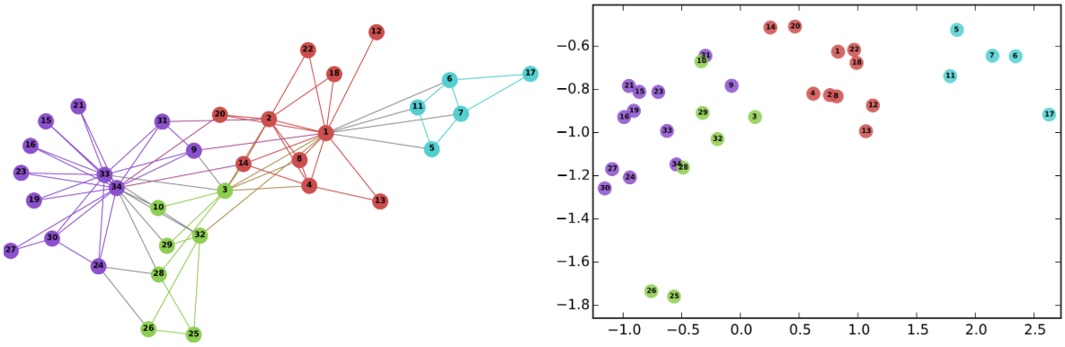
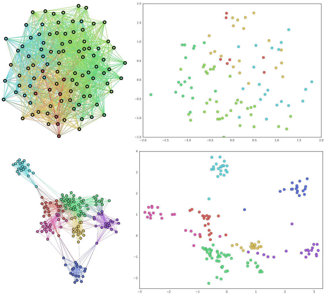
Graph Matching Networks for Learning the Similarity of Graph Structured Objects
Yujia Li, Chenjie Gu, Thomas Dullien, Oriol Vinyals, Pushmeet Kohli

Subspace Robust Wasserstein Distances
François-Pierre Paty, Marco Cuturi

Training Well-Generalizing Classifiers for Fairness Metrics and Other Data-Dependent Constraints
Andrew Cotter, Maya Gupta, Heinrich Jiang, Nathan Srebro, Karthik Sridharan, Serena Wang, Blake Woodworth, Seungil You

The Effect of Network Width on Stochastic Gradient Descent and Generalization: an Empirical Study
Daniel Park, Jascha Sohl-Dickstein, Quoc Le, Samuel Smith

A Theory of Regularized Markov Decision Processes
Matthieu Geist, Bruno Scherrer, Olivier Pietquin

Area Attention
Yang Li, Łukasz Kaiser, Samy Bengio, Si Si

EfficientNet: Rethinking Model Scaling for Convolutional Neural Networks
Mingxing Tan, Quoc Le

Static Automatic Batching In TensorFlow
Ashish Agarwal

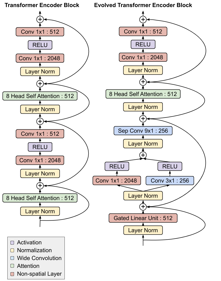
The Evolved Transformer
David So, Quoc Le, Chen Liang

Policy Certificates: Towards Accountable Reinforcement Learning
Christoph Dann, Lihong Li, Wei Wei, Emma Brunskill

Self-similar Epochs: Value in Arrangement
Eliav Buchnik, Edith Cohen, Avinatan Hasidim, Yossi Matias

The Value Function Polytope in Reinforcement Learning
Robert Dadashi, Marc G. Bellemare, Adrien Ali Taiga, Nicolas Le Roux, Dale Schuurmans

Adversarial Examples Are a Natural Consequence of Test Error in Noise
Justin Gilmer, Nicolas Ford, Nicholas Carlini, Ekin Cubuk

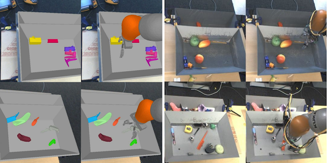
SOLAR: Deep Structured Representations for Model-Based Reinforcement Learning
Marvin Zhang, Sharad Vikram, Laura Smith, Pieter Abbeel, Matthew Johnson, Sergey Levine

Garbage In, Reward Out: Bootstrapping Exploration in Multi-Armed Bandits
Branislav Kveton, Csaba Szepesvari, Sharan Vaswani, Zheng Wen, Tor Lattimore, Mohammad Ghavamzadeh

Imperceptible, Robust, and Targeted Adversarial Examples for Automatic Speech Recognition
Yao Qin, Nicholas Carlini, Garrison Cottrell, Ian Goodfellow, Colin Raffel

Direct Uncertainty Prediction for Medical Second Opinions
Maithra Raghu, Katy Blumer, Rory Sayres, Ziad Obermeyer, Bobby Kleinberg, Sendhil Mullainathan, Jon Kleinberg

A Large-Scale Study on Regularization and Normalization in GANs
Karol Kurach, Mario Lučić, Xiaohua Zhai, Marcin Michalski, Sylvain Gelly

Learning a Compressed Sensing Measurement Matrix via Gradient Unrolling
Shanshan Wu, Alex Dimakis, Sujay Sanghavi, Felix Yu, Daniel Holtmann-Rice, Dmitry Storcheus, Afshin Rostamizadeh, Sanjiv Kumar

NATTACK: Learning the Distributions of Adversarial Examples for an Improved Black-Box Attack on Deep Neural Networks
Yandong Li, Lijun Li, Liqiang Wang, Tong Zhang, Boqing Gong

Distributed Weighted Matching via Randomized Composable Coresets
Sepehr Assadi, Mohammad Hossein Bateni, Vahab Mirrokni

Monge blunts Bayes: Hardness Results for Adversarial Training
Zac Cranko, Aditya Menon, Richard Nock, Cheng Soon Ong, Zhan Shi, Christian Walder

Generalized Majorization-Minimization
Sobhan Naderi Parizi, Kun He, Reza Aghajani, Stan Sclaroff, Pedro Felzenszwalb

NAS-Bench-101: Towards Reproducible Neural Architecture Search
Chris Ying, Aaron Klein, Eric Christiansen, Esteban Real, Kevin Murphy, Frank Hutter

Variational Russian Roulette for Deep Bayesian Nonparametrics
Kai Xu, Akash Srivastava, Charles Sutton

Surrogate Losses for Online Learning of Stepsizes in Stochastic Non-Convex Optimization
Zhenxun Zhuang, Ashok Cutkosky, Francesco Orabona

Improved Parallel Algorithms for Density-Based Network Clustering
Mohsen Ghaffari, Silvio Lattanzi, Slobodan Mitrović

The Advantages of Multiple Classes for Reducing Overfitting from Test Set Reuse
Vitaly Feldman, Roy Frostig, Moritz Hardt

Submodular Streaming in All Its Glory: Tight Approximation, Minimum Memory and Low Adaptive Complexity
Ehsan Kazemi, Marko Mitrovic, Morteza Zadimoghaddam, Silvio Lattanzi, Amin Karbasi

Hiring Under Uncertainty
Manish Purohit, Sreenivas Gollapudi, Manish Raghavan

A Tree-Based Method for Fast Repeated Sampling of Determinantal Point Processes
Jennifer Gillenwater, Alex Kulesza, Zelda Mariet, Sergei Vassilvtiskii

Statistics and Samples in Distributional Reinforcement Learning
Mark Rowland, Robert Dadashi, Saurabh Kumar, Remi Munos, Marc G. Bellemare, Will Dabney

Provably Efficient Maximum Entropy Exploration
Elad Hazan, Sham Kakade, Karan Singh, Abby Van Soest

Active Learning with Disagreement Graphs
Corinna Cortes, Giulia DeSalvo,, Mehryar Mohri, Ningshan Zhang, Claudio Gentile

MixHop: Higher-Order Graph Convolutional Architectures via Sparsified Neighborhood Mixing
Sami Abu-El-Haija, Bryan Perozzi, Amol Kapoor, Nazanin Alipourfard, Kristina Lerman, Hrayr Harutyunyan, Greg Ver Steeg, Aram Galstyan

Understanding the Impact of Entropy on Policy Optimization
Zafarali Ahmed, Nicolas Le Roux, Mohammad Norouzi, Dale Schuurmans

Matrix-Free Preconditioning in Online Learning
Ashok Cutkosky, Tamas Sarlos

State-Reification Networks: Improving Generalization by Modeling the Distribution of Hidden Representations
Alex Lamb, Jonathan Binas, Anirudh Goyal, Sandeep Subramanian, Ioannis Mitliagkas, Yoshua Bengio, Michael Mozer

Online Convex Optimization in Adversarial Markov Decision Processes
Aviv Rosenberg, Yishay Mansour

Bounding User Contributions: A Bias-Variance Trade-off in Differential Privacy
Kareem Amin, Alex Kulesza, Andres Munoz Medina, Sergei Vassilvtiskii

Complementary-Label Learning for Arbitrary Losses and Models
Takashi Ishida, Gang Niu, Aditya Menon, Masashi Sugiyama

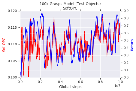
Learning Latent Dynamics for Planning from Pixels
Danijar Hafner, Timothy Lillicrap, Ian Fischer, Ruben Villegas, David Ha, Honglak Lee, James Davidson

Unifying Orthogonal Monte Carlo Methods
Krzysztof Choromanski, Mark Rowland, Wenyu Chen, Adrian Weller

Differentially Private Learning of Geometric Concepts
Haim Kaplan, Yishay Mansour, Yossi Matias, Uri Stemmer

Online Learning with Sleeping Experts and Feedback Graphs
Corinna Cortes, Giulia DeSalvo, Claudio Gentile, Mehryar Mohri, Scott Yang

Adaptive Scale-Invariant Online Algorithms for Learning Linear Models
Michal Kempka, Wojciech Kotlowski, Manfred K. Warmuth

TensorFuzz: Debugging Neural Networks with Coverage-Guided Fuzzing
Augustus Odena, Catherine Olsson, David Andersen, Ian Goodfellow

Online Control with Adversarial Disturbances
Naman Agarwal, Brian Bullins, Elad Hazan, Sham Kakade, Karan Singh

Adversarial Online Learning with Noise
Alon Resler, Yishay Mansour

Escaping Saddle Points with Adaptive Gradient Methods
Matthew Staib, Sashank Reddi, Satyen Kale, Sanjiv Kumar, Suvrit Sra

Fairness Risk Measures
Robert Williamson, Aditya Menon

DBSCAN++: Towards Fast and Scalable Density Clustering
Jennifer Jang, Heinrich Jiang

Learning Linear-Quadratic Regulators Efficiently with only √T Regret
Alon Cohen, Tomer Koren, Yishay Mansour

Understanding and correcting pathologies in the training of learned optimizers
Luke Metz, Niru Maheswaranathan, Jeremy Nixon, Daniel Freeman, Jascha Sohl-Dickstein

Parameter-Efficient Transfer Learning for NLP
Neil Houlsby, Andrei Giurgiu, Stanislaw Jastrzebski, Bruna Morrone, Quentin De Laroussilhe, Andrea Gesmundo, Mona Attariyan, Sylvain Gelly

Efficient Full-Matrix Adaptive Regularization
Naman Agarwal, Brian Bullins, Xinyi Chen, Elad Hazan, Karan Singh, Cyril Zhang, Yi Zhang

Efficient On-Device Models Using Neural Projections
Sujith Ravi

Flexibly Fair Representation Learning by Disentanglement
Elliot Creager, David Madras, Joern-Henrik Jacobsen, Marissa Weis, Kevin Swersky, Toniann Pitassi, Richard Zemel

Recursive Sketches for Modular Deep Learning
Badih Ghazi, Rina Panigrahy, Joshua Wang

POLITEX: Regret Bounds for Policy Iteration Using Expert Prediction
Yasin Abbasi-Yadkori, Peter L. Bartlett, Kush Bhatia, Nevena Lazić, Csaba Szepesvári, Gellért Weisz

Anytime Online-to-Batch, Optimism and Acceleration
Ashok Cutkosky

Insertion Transformer: Flexible Sequence Generation via Insertion Operations
Mitchell Stern, William Chan, Jamie Kiros, Jakob Uszkoreit

Robust Inference via Generative Classifiers for Handling Noisy Labels
Kimin Lee, Sukmin Yun, Kibok Lee, Honglak Lee, Bo Li, Jinwoo Shin

A Better k-means++ Algorithm via Local Search
Silvio Lattanzi, Christian Sohler

Analyzing and Improving Representations with the Soft Nearest Neighbor Loss
Nicholas Frosst, Nicolas Papernot, Geoffrey Hinton

Learning to Generalize from Sparse and Underspecified Rewards
Rishabh Agarwal, Chen Liang, Dale Schuurmans, Mohammad Norouzi

MeanSum: A Neural Model for Unsupervised Multi-Document Abstractive Summarization
Eric Chu, Peter Liu

CHiVE: Varying Prosody in Speech Synthesis with a Linguistically Driven Dynamic Hierarchical Conditional Variational Network
Tom Kenter, Vincent Wan, Chun-An Chan, Rob Clark, Jakub Vit

Similarity of Neural Network Representations Revisited
Simon Kornblith, Mohammad Norouzi, Honglak Lee, Geoffrey Hinton

Online Algorithms for Rent-Or-Buy with Expert Advice
Sreenivas Gollapudi, Debmalya Panigrahi

Breaking the Softmax Bottleneck via Learnable Monotonic Pointwise Non-linearities
Octavian Ganea, Sylvain Gelly, Gary Becigneul, Aliaksei Severyn

Non-monotone Submodular Maximization with Nearly Optimal Adaptivity and Query Complexity
Matthew Fahrbach, Vahab Mirrokni, Morteza Zadimoghaddam

Agnostic Federated Learning
Mehryar Mohri, Gary Sivek, Ananda Theertha Suresh

Categorical Feature Compression via Submodular Optimization
Mohammad Hossein Bateni, Lin Chen, Hossein Esfandiari, Thomas Fu, Vahab Mirrokni, Afshin Rostamizadeh

Cross-Domain 3D Equivariant Image Embeddings
Carlos Esteves, Avneesh Sud, Zhengyi Luo, Kostas Daniilidis, Ameesh Makadia

Faster Algorithms for Binary Matrix Factorization
Ravi Kumar, Rina Panigrahy, Ali Rahimi, David Woodruff

On Variational Bounds of Mutual Information
Ben Poole, Sherjil Ozair, Aaron Van Den Oord, Alex Alemi, George Tucker

Guided Evolutionary Strategies: Augmenting Random Search with Surrogate Gradients
Niru Maheswaranathan, Luke Metz, George Tucker, Dami Choi, Jascha Sohl-Dickstein

Semi-Cyclic Stochastic Gradient Descent
Hubert Eichner, Tomer Koren, Brendan McMahan, Nathan Srebro, Kunal Talwar

Workshops
1st Workshop on Understanding and Improving Generalization in Deep Learning
Organizers Include: Dilip Krishnan, Hossein Mobahi
Invited Speaker: Chelsea Finn

Climate Change: How Can AI Help?
Invited Speaker: John Platt

Generative Modeling and Model-Based Reasoning for Robotics and AI
Organizers Include: Dumitru Erhan, Sergey Levine, Kimberly Stachenfeld
Invited Speaker: Chelsea Finn

Human In the Loop Learning (HILL)
Organizers Include: Been Kim

ICML 2019 Time Series Workshop
Organizers Include: Vitaly Kuznetsov

Joint Workshop on On-Device Machine Learning & Compact Deep Neural Network Representations (ODML-CDNNR)
Organizers Include: Sujith Ravi, Zornitsa Kozareva

Negative Dependence: Theory and Applications in Machine Learning
Organizers Include: Jennifer Gillenwater, Alex Kulesza

Reinforcement Learning for Real Life
Organizers Include: Lihong Li
Invited Speaker: Craig Boutilier

Uncertainty and Robustness in Deep Learning
Organizers Include: Justin Gilmer

Theoretical Physics for Deep Learning
Organizers Include: Jaehoon Lee, Jeffrey Pennington, Yasaman Bahri

Workshop on the Security and Privacy of Machine Learning
Organizers Include: Nicolas Papernot
Invited Speaker: Been Kim

Exploration in Reinforcement Learning Workshop
Organizers Include: Benjamin Eysenbach, Surya Bhupatiraju, Shixiang Gu

ICML Workshop on Imitation, Intent, and Interaction (I3)
Organizers Include: Sergey Levine, Chelsea Finn
Invited Speaker: Pierre Sermanet

Identifying and Understanding Deep Learning Phenomena
Organizers Include: Hanie Sedghi, Samy Bengio, Kenji Hata, Maithra Raghu, Ali Rahimi, Ying Xiao

Workshop on Multi-Task and Lifelong Reinforcement Learning
Organizers Include: Sarath Chandar, Chelsea Finn
Invited Speakers: Karol Hausman, Sergey Levine

Workshop on Self-Supervised Learning
Organizers Include: Pierre Sermanet

Invertible Neural Networks and Normalizing Flows
Organizers Include: Rianne Van den Berg, Danilo J. Rezende
Invited Speakers: Eric Jang, Laurent Dinh

Posted by Karol Kurach, Research Lead and Olivier Bachem, Research Scientist, Google Research, Zürich

The goal of reinforcement learning (RL) is to train smart agents that can interact with their environment and solve complex tasks, with real-world applications towards robotics, self-driving cars, and more. The rapid progress in this field has been fueled by making agents play games such as the iconic Atari console games, the ancient game of Go, or professionally played video games like Dota 2 or Starcraft 2, all of which provide challenging environments where new algorithms and ideas can be quickly tested in a safe and reproducible manner. The game of football is particularly challenging for RL, as it requires a natural balance between short-term control, learned concepts, such as passing, and high level strategy.

Today we are happy to announce the release of the Google Research Football Environment, a novel RL environment where agents aim to master the world’s most popular sport—football. Modeled after popular football video games, the Football Environment provides a physics based 3D football simulation where agents control either one or all football players on their team, learn how to pass between them, and manage to overcome their opponent’s defense in order to score goals. The Football Environment provides several crucial components: a highly-optimized game engine, a demanding set of research problems called Football Benchmarks, as well as the Football Academy, a set of progressively harder RL scenarios. In order to facilitate research, we have released a beta version of the underlying open-source code on Github.

Football Engine
The core of the Football Environment is an advanced football simulation, called Football Engine, which is based on a heavily modified version of Gameplay Football. Based on input actions for the two opposing teams, it simulates a match of football including goals, fouls, corner and penalty kicks, and offsides. The Football Engine is written in highly optimized C++ code, allowing it to be run on off-the-shelf machines, both with GPU and without GPU-based rendering enabled. This allows it to reach a performance of approximately 25 million steps per day on a single hexa-core machine.

The Football Engine is an advanced football simulation that supports all the major football rules such as kickoffs (top left), goals (top right), fouls, cards (bottom left), corner and penalty kicks (bottom right), and offside.

The Football Engine has additional features geared specifically towards RL. First, it allows learning from both different state representations, which contain semantic information such as the player’s locations, as well as learning from raw pixels. Second, to investigate the impact of randomness, it can be run in both a stochastic mode (enabled by default), in which there is randomness in both the environment and opponent AI actions, and in a deterministic mode, where there is no randomness. Third, the Football Engine is out of the box compatible with the widely used OpenAI Gym API. Finally, researchers can get a feeling for the game by playing against each other or their agents, using either keyboards or gamepads.

Football Benchmarks
With the Football Benchmarks, we propose a set of benchmark problems for RL research based on the Football Engine. The goal in these benchmarks is to play a “standard” game of football against a fixed rule-based opponent that was hand-engineered for this purpose. We provide three versions: the Football Easy Benchmark, the Football Medium Benchmark, and the Football Hard Benchmark, which only differ in the strength of the opponent.

As a reference, we provide benchmark results for two state-of-the-art reinforcement learning algorithms: DQN and IMPALA, which both can be run in multiple processes on a single machine or concurrently on many machines. We investigate both the setting where the only rewards provided to the algorithm are the goals scored and the setting where we provide additional rewards for moving the ball closer to the goal.

Our results indicate that the Football Benchmarks are interesting research problems of varying difficulties. In particular, the Football Easy Benchmark appears to be suitable for research on single-machine algorithms while the Football Hard Benchmark proves to be challenging even for massively distributed RL algorithms. Based on the nature of the environment and the difficulty of the benchmarks, we expect them to be useful for investigating current scientific challenges such as sample-efficient RL, sparse rewards, or model based RL.

The average goal difference of agent versus opponent at different difficulty levels for different baselines. The Easy opponent can be beaten by a DQN agent trained for 20 million steps, while the Medium and Hard opponents require a distributed algorithm such as IMPALA that is trained for 200 million steps.

Football Academy & Future Directions
As training agents for the full Football Benchmarks can be challenging, we also provide Football Academy, a diverse set of scenarios of varying difficulty. This allows researchers to get the ball rolling on new research ideas, allows testing of high-level concepts (such as passing), and provides a foundation to investigate curriculum learning research ideas, where agents learn from progressively harder scenarios. Examples of the Football Academy scenarios include settings where agents have to learn how to score against the empty goal, where they have to learn how to quickly pass between players, and where they have to learn how to execute a counter-attack. Using a simple API, researchers can further define their own scenarios and train agents to solve them.

Top: A successful policy that runs towards the goal (as required, since a number of opponents chase our player) and scores against the goal-keeper. Second: A beautiful way to drive and finish a counter-attack. Third: A simple way to solve a 2-vs-1 play. Bottom: The agent scores after a corner kick.

The Football Benchmarks and the Football Academy consider the standard RL setup, in which agents compete against a fixed opponent, i.e., where the opponent can be considered a part of the environment. Yet, in reality, football is a two-player game where two different teams compete and where one has to adapt to the actions and strategy of the opposing team. The Football Engine provides a unique opportunity for research into this setting and, once we complete our on-going effort to implement self-play, even more interesting research settings can be investigated.

Acknowledgments
This project was undertaken together with Anton Raichuk, Piotr Stańczyk, Michał Zając, Lasse Espeholt, Carlos Riquelme, Damien Vincent‎, Marcin Michalski, Olivier Bousquet‎ and Sylvain Gelly at Google Research, Zürich. We also wish to thank Lucas Beyer, Nal Kalchbrenner, Tim Salimans and the rest of the Google Brain team for helpful discussions, comments, technical help and code contributions. Finally, we would like to thank Bastiaan Konings Schuiling, who authored and open-sourced the original version of this game.

Posted by Paul Dille, Senior Software Developer, Carnegie Mellon University CREATE Lab, and Chris Herwig, Geo Data Engineer, Google Earth Outreach

Six years ago, we first introduced Google Earth Timelapse, a global, zoomable time-lapse video that lets anyone explore our changing planet’s surface—from the global scale to the local scale. Earth Timelapse consists of 83 million multi-resolution overlapping video tiles, which are made interactively explorable through the open-source Time Machine client software developed at Carnegie Mellon University’s CREATE Lab. At its core, Google Earth Timelapse is an example of how organizing information can make it more accessible and useful, turning petabytes of satellite imagery into an interactive experience that shows the dynamic changes occurring across space and time.

In April, we introduced several updates to Timelapse, including two additional years of imagery to the time-series visualization, which now spans from 1984 to 2018, with visual upgrades that make exploring more accessible and intuitive. We are especially excited that this update includes support for mobile and tablet devices, which are quickly overtaking desktop computers as the dominant source of app traffic.

Building the Global Visualization
Making a planetary-sized time-lapse video required a significant amount of pixel crunching in Earth Engine, Google’s cloud platform for petabyte-scale geospatial analysis. The new release followed a process similar to what we did in 2013, but at a significantly greater scale—turning 15 million satellite images acquired over the last three and a half decades from the USGS/NASA Landsat and European Sentinel programs into 35 cloud-free 4-terapixel images of the planet—one for each year from 1984 to 2018.

At its native resolution, the Timelapse visualization is a 4 terapixel video (that’s four trillion pixels), which would take about 12 days to download on a 95 Mb/s internet connection. Most computers would have difficulty playing a video of this size, let alone with an interactive, zoomable interface. The problem is even more severe for a mobile device.

A solution was pioneered by Google Maps in 2004 with the map pyramiding technique. Before that time, navigating a map required the use of directional arrows to pan and zoom, with each step requiring the page to reload. The map pyramiding technique assembles the full map image displayed on-screen from tens of small 256×256 pixel non-overlapping image tiles in an array, with new tiles fetched as needed at an appropriate resolution as the user pans and zooms across the map.

A traditional Mercator map pyramid contains non-overlapping image tiles.

This works very well for maps made of static images, but less so for pyramids of video tiles, such as those used by Timelapse, since it requires a web browser to keep up to 16 videos in sync while interacting with the visualization. The solution is embodied in CREATE Lab’s open source Time Machine software: create much larger video tiles that can cover the entire screen and only show one whole-screen tile at a time. The tiles create a pyramid, where sibling tiles overlap with their neighbors to provide a seamless transition between tiles while panning and zooming. Though the overlapping tiles require the use of about 16x more videos, this pyramid structure enables the use of Timelapse on mobile devices by minimizing the amount of data required for visualization.

In our newest release, the global video pyramid consists of 83 million videos across 13 zoom levels, which required about 2 million CPU hours distributed across thousands of machines in Google Cloud to generate.

Earth Timelapse uses a pyramid of overlapping video tiles.

Time Travel, Wherever You Are
Prior to April’s update, ~30% of visitors to the Timelapse visualization were on mobile devices and didn’t actually experience the visualization; instead they saw a YouTube playlist of locations in Timelapse. Until recently, the hardware and CPUs for phones and tablets could not decode videos fast enough without significant delays when someone attempted to zoom in or pan across a video, making mobile exploration unpleasant, if not impossible. In addition, in order for the visualization to be smooth as you pan and zoom, each video that is loaded must sync to the previously playing video and begin playing automatically. But, until only recently, mobile browser vendors had disabled video autoplay at the browser level for bandwidth reasons.

Now that mobile browser vendors have re-enabled video autoplay, we are able to take advantage of current mobile hardware and CPU capabilities, while leveraging the pyramid mapping technique’s efficient use of data, to enable Timelapse on mobile.

Redesigning Timelapse for Exploration Across Devices
Timelapse is a tool for exploration, so we designed for immersiveness, devoting as much real estate as possible to the map. On the other hand, it’s not just a map, but a map of videos. So we kept controls visible, like pausing and restarting the timeline or choosing highlights, by leveraging Material Design with simple, clean lines and clear focal areas.

Navigate with Google Maps using the new “Maps Mode” toggle.

To explore, you need to know where you are or where somewhere else is, so the new interface includes a new “Maps Mode” toggle that lets the user navigate with Google Maps. We also built in scalability to the timeline element of the UI, so that new features added in the future, such as lengthening the time-lapse or adding options for different time increments, won’t break the design. The timeline also allows the user to go backwards in time—an interesting way to compare the present with the past.

For desktop browsers supporting WebGL, we also added a new WebGL viewer to the open source project, which loads and synchronizes multiple videos to fill the screen at optimal resolution. The aesthetic improvement of this is nontrivial, with >4x better resolution.

What’s next
We’re excited about the abundance of freely available, openly licensed satellite imagery and remote sensing data available, enabling new visualizations across time, space, and the visual and non-visual spectrum. We’ve found it’s often the data combined with supplemental layers, such as the World Database on Protected Areas (WDPA) boundaries, that can spark new insights. For example, seeing the visual connection between declining home ownership and shifts in the city of Pittsburgh’s racial makeup tells a story about inequality that numbers on a page simply cannot. Visual evidence can transcend language and cultural barriers and, we hope, generate productive conversations about our global challenges.

Acknowledgements
Randy Sargent, Senior Systems Scientist, Carnegie Mellon University CREATE Lab and the Google Earth Engine team

Posted by Chase Roberts, Research Engineer, Google AI and Stefan Leichenauer, Research Scientist, X

Many of the world’s toughest scientific challenges, like developing high-temperature superconductors and understanding the true nature of space and time, involve dealing with the complexity of quantum systems. What makes these challenges difficult is that the number of quantum states in these systems is exponentially large, making brute-force computation infeasible. To deal with this, data structures called tensor networks are used. Tensor networks let one focus on the quantum states that are most relevant for real-world problems—the states of low energy, say—while ignoring other states that aren’t relevant. Tensor networks are also increasingly finding applications in machine learning (ML). However, there remain difficulties that prohibit them from widespread use in the ML community: 1) a production-level tensor network library for accelerated hardware has not been available to run tensor network algorithms at scale, and 2) most of the tensor network literature is geared toward physics applications and creates the false impression that expertise in quantum mechanics is required to understand the algorithms.

In order to address these issues, we are releasing TensorNetwork, a brand new open source library to improve the efficiency of tensor calculations, developed in collaboration with the Perimeter Institute for Theoretical Physics and X. TensorNetwork uses TensorFlow as a backend and is optimized for GPU processing, which can enable speedups of up to 100x when compared to work on a CPU. We introduce TensorNetwork in a series of papers, the first of which presents the new library and its API, and provides an overview of tensor networks for a non-physics audience. In our second paper we focus on a particular use case in physics, demonstrating the speedup that one gets using GPUs.

How are Tensor Networks Useful?
Tensors are multidimensional arrays, categorized in a hierarchy according to their order: e.g., an ordinary number is a tensor of order zero (also known as a scalar), a vector is an order-one tensor, a matrix is an order-two tensor, and so on. While low-order tensors can easily be represented by an explicit array of numbers or with a mathematical symbol such as T_ijnklm (where the number of indices represents the order of the tensor), that notation becomes very cumbersome once we start talking about high-order tensors. At that point it’s useful to start using diagrammatic notation, where one simply draws a circle (or some other shape) with a number of lines, or legs, coming out of it—the number of legs being the same as the order of the tensor. In this notation, a scalar is just a circle, a vector has a single leg, a matrix has two legs, etc. Each leg of the tensor also has a dimension, which is the size of that leg. For example, a vector representing an object’s velocity through space would be a three-dimensional, order-one tensor.

Diagrammatic notation for tensors.

The benefit of representing tensors in this way is to succinctly encode mathematical operations, e.g., multiplying a matrix by a vector to produce another vector, or multiplying two vectors to make a scalar. These are all examples of a more general concept called tensor contraction.

Diagrammatic notation for tensor contraction. Vector and matrix multiplication, as well as the matrix trace (i.e., the sum of the diagonal elements of a matrix), are all examples.

These are also simple examples of tensor networks, which are graphical ways of encoding the pattern of tensor contractions of several constituent tensors to form a new one. Each constituent tensor has an order determined by its own number of legs. Legs that are connected, forming an edge in the diagram, represent contraction, while the number of remaining dangling legs determines the order of the resultant tensor.

Left: The trace of the product of four matrices, tr(ABCD), which is a scalar. You can see that it has no dangling legs. Right: Three order-three tensors being contracted with three legs dangling, resulting in a new order-three tensor.

While these examples are very simple, the tensor networks of interest often represent hundreds of tensors contracted in a variety of ways. Describing such a thing would be very obscure using traditional notation, which is why the diagrammatic notation was invented by Roger Penrose in 1971.

Tensor Networks in Practice
Consider a collection of black-and-white images, each of which can be thought of as a list of N pixel values. A single pixel of a single image can be one-hot-encoded into a two-dimensional vector, and by combining these pixel encodings together we can make a 2^N-dimensional one-hot encoding of the entire image. We can reshape that high-dimensional vector into an order-N tensor, and then add up all of the tensors in our collection of images to get a total tensor T_i1,i2,…,iN encapsulating the collection.

This sounds like a very wasteful thing to do: encoding images with about 50 pixels in this way would already take petabytes of memory. That’s where tensor networks come in. Rather than storing or manipulating the tensor T directly, we instead represent T as the contraction of many smaller constituent tensors in the shape of a tensor network. That turns out to be much more efficient. For instance, the popular matrix product state (MPS) network would write T in terms of N much smaller tensors, so that the total number of parameters is only linear in N, rather than exponential.

The high-order tensor T is represented in terms of many low-order tensors in a matrix product state tensor network.

It’s not obvious that large tensor networks can be efficiently created or manipulated while consistently avoiding the need for a huge amount of memory. But it turns out that this is possible in many cases, which is why tensor networks have been used extensively in quantum physics and, now, in machine learning. Stoudenmire and Schwab used the encoding just described to make an image classification model, demonstrating a new use for tensor networks. The TensorNetwork library is designed to facilitate exactly that kind of work, and our first paper describes how the library functions for general tensor network manipulations.

Performance in Physics Use-Cases
TensorNetwork is a general-purpose library for tensor network algorithms, and so it should prove useful for physicists as well. Approximating quantum states is a typical use-case for tensor networks in physics, and is well-suited to illustrate the capabilities of the TensorNetwork library. In our second paper, we describe a tree tensor network (TTN) algorithm for approximating the ground state of either a periodic quantum spin chain (1D) or a lattice model on a thin torus (2D), and implement the algorithm using TensorNetwork. We compare the use of CPUs with GPUs and observe significant computational speed-ups, up to a factor of 100, when using a GPU and the TensorNetwork library.

Computational time as a function of the bond dimension, χ. The bond dimension determines the size of the constituent tensors of the tensor network. A larger bond dimension means the tensor network is more powerful, but requires more computational resources to manipulate.

Conclusion and Future Work
These are the first in a series of planned papers to illustrate the power of TensorNetwork in real-world applications. In our next paper we will use TensorNetwork to classify images in the MNIST and Fashion-MNIST datasets. Future plans include time series analysis on the ML side, and quantum circuit simulation on the physics side. With the open source community, we are also always adding new features to TensorNetwork itself. We hope that TensorNetwork will become a valuable tool for physicists and machine learning practitioners.

Acknowledgements
The TensorNetwork library was developed by Chase Roberts, Adam Zalcman, and Bruce Fontaine of Google AI; Ashley Milsted, Martin Ganahl, and Guifre Vidal of the Perimeter Institute; and Jack Hidary and Stefan Leichenauer of X. We’d also like to thank Stavros Efthymiou at X for valuable contributions.