In this blog post, we’re introducing the Amazon SageMaker Object2Vec algorithm, a new highly customizable multi-purpose algorithm that can learn low dimensional dense embeddings of high dimensional objects.
Embeddings are an important feature engineering technique in machine learning (ML). They convert high dimensional vectors into low-dimensional space to make it easier to do machine learning with large sparse vector inputs. Embeddings also capture the semantics of the underlying data by placing similar items closer in the low-dimensional space. This makes the features more effective in training downstream models. One of the well-known embedding techniques is Word2Vec, which provides embeddings for words. It has been widely used in many use cases, such as sentiment analysis, document classification, and natural language understanding. See the following diagram for a conceptual representation of word embeddings in the feature space.

Figure 1: Word2Vec embeddings: words that are semantically similar are close together in the embedding space.
In addition to word embeddings, there are also use cases where we want to learn the embeddings of more general-purpose objects such as sentences, customers, and products. This is so we can build practical applications for information retrieval, product search, item matching, customer profiling based on similarity or as inputs for other supervised tasks. This is where Amazon SageMaker Object2Vec comes in. In this blog post, we will talk about what it is, how it works, discuss some practical use cases, and show you how Object2Vec can be used to solve those use cases.
How it works
The embeddings are learned such that the semantics of the relationship between pairs of objects in the original space are preserved in the embedding space. Thus, the learned embeddings can be used to efficiently compute nearest neighbors of objects, as well as to visualize natural clusters of related objects in low-dimensional space. In addition, the embeddings can also be used as features of the corresponding objects in downstream supervised tasks such as classification or regression.
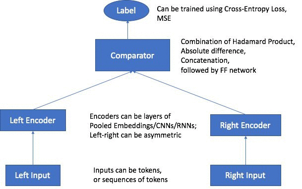
The architecture of Amazon SageMaker Object2Vec consists of the following main components:
- 2 input channels—The two input channels take object pairs of same or different types as inputs and pass them to independent and customizable encoders. Examples of input objects could be sequence pairs, tokens pairs, and sequence and tokens pairs.
- 2 encoders—The encoders convert each object into a fixed-length embedding vector. The encoded embeddings of the objects in the pair are then passed into a comparator.
- Comparator—The comparator compares the embeddings in different ways and outputs scores that correspond to the strength of the relationship of the objects in the pair for each relationship type specified by the user. An example of the output score could be 1, indicating a strong relationship between the pair of objects, or 0, representing a weak relationship.
At training time, the training loss function minimizes the differences between the relationships predicted by the model and those specified by the user in the training data. After the model is trained, the trained encoder can be used to convert new input objects into fixed-length embeddings. The architectural diagram of Object2Vec and an explanation of the parts of the architecture follows.
Supported input types, encoders and loss functions
Natively, Object2Vec currently supports singleton discrete tokens represented as integer-ids as well as sequences of discrete tokens represented as lists of integer-ids as inputs, so pre-processing is required to transform the input data to the supported formats. The objects in each pair can be asymmetric with respect to each other. For example, they can be (token, sequence) pairs, or (token, token) pairs, or (sequence, sequence) pairs. For tokens, we support simple embeddings as compatible encoders, while for sequences of tokens, we support average-pooled embeddings, hierarchical Convolutional Neural Networks (CNNs), as well as multi-layered Bi-Directional-Long-Short-Term-Memory (BiLSTM)-based Recurrent Neural Networks as encoders. The input label for each pair can be a categorical label that expresses the relationship between the objects in the pair, or it can be a rating or a score that expresses the strength of similarity between the two objects. For categorical labels, we support Cross-Entropy loss function, and for ratings/score-based labels, we support Mean Squared Error (MSE) loss function.
Although the current input types supported in Object2Vec are either sequences of discrete tokens or singleton tokens, these input types already cover plenty of real-world objects since the data that describes these objects can usually be represented as discrete sequences. Here are a few illustrative examples:
- Embeddings of customers: To learn the embeddings of customers, you can generate training data consisting of a recent sequence of transactions of each customer, where the sequence is represented as the list of product-IDs bought by the customer, paired with the ID of the customer, as positive examples. As negative examples, one can generate transactions of a different customer paired with the original (and therefore incorrect) customer-ID. For each pair, the sequence of transactions could be passed as input to a CNN or BiLSTM encoder, and the customer-ID to an embedding-based encoder. Once trained, the embeddings of the customers can be directly read from the embedding-based encoder.
- Embeddings of products: To train embeddings of products, you can pair the title of the product, represented as a sequence of text tokens, and the product-ID as positive examples. As negative examples, one can pair title of another (potentially related) product with the original (and incorrect) product-ID.
- Embeddings of users and movies: To train embeddings of users and movies, you can use user-movie pairs where the user has assigned a high rating to the movie as positive examples, and those that the user has assigned low rating as negative examples. You can use an embedding-based encoder for both users and movies, and the embeddings of either can be read directly from the corresponding encoder, once trained.
- Embeddings of football players: To learn the embeddings of players in a football game, you can use the time sequence of discretized locations in the field traced by each player during a game, paired with the player-ID as positive examples. Traced location sequences of a player paired with a different player-ID can serve as negative examples.
- Embeddings of English sentences: To learn embeddings of sentences in English, you can treat pairs of adjacent sentences in a document as positive pairs, and the pairs of sentences sampled from different documents as negative pairs. You can use CNN- or BiLSTM-based encoders for both sentences in the pair. Once trained, either encoder can be used to generate embeddings of new sentences.
In this blog post we’ll walk through some of these use cases in more detail using our Jupyter Notebook examples (movie recommendation, multi-label document classification, and sentence similarity).
Is Object2Vec a supervised learning algorithm?
Since the algorithm requires labeled data for training, it is indeed true that Object2Vec is a supervised learner. However, we want to emphasize that there are many scenarios where the relationship labels can be obtained purely from natural clusterings in data, without any explicit human annotation. We discussed some examples earlier, but we reiterate them as follows for clarity.
- To learn embeddings of words, pairs of words that occur within a context window in a given document can be considered examples with a positive label and word pairs obtained as samples from unigram distribution in a corpus can be considered as examples with a negative label.
- Likewise, to learn embeddings of sentences, pairs of sentences that occur adjacent to each other in a document can be considered examples with “positive labels” and sentence pairs that do not co-occur in the same document can be considered as those with negative labels.”
- To learn embeddings of a customer, pairs of transaction records from the same customer within a given window of time can be considered positive examples, and pairs of transactions from two different customers can be considered negative examples.
To reiterate, the architecture of Object2Vec requires the user to make the relationship between objects in each pair explicit at training time, but the relationships themselves may be obtained from natural groupings in data, and they might not require explicit human labeling.
Hyperparameter
Object2Vec supports a range of hyperparameters for fine-tuning the training to meet different requirements. These are some of the main hyperparameters:
- Encoder network (network)– You can choose Hierarchical CNN, BiLSTM, or Pooled Embedding. Use Hierarchical CNN if you want faster training speed due to parallelization. BiLSTM will give you better results for sequential inputs, such as sentences where long-distance dependencies between tokens in the sequence need to be captured. Pooled embedding is designed for the super-fast training at the cost of some drop in accuracy.
- Optimizer– You can choose among ‘adam’ ‘adagrad,’ ‘rmsprop,’ ‘sgd,’ and ‘adadelta.’
- Token embedding dimension (token_embedding_dim) – The dimension of the input layer. This is the layer where pre-trained embeddings could be applied.
- Encoding dimension (enc_dim) – The dimension of the final encoding of the input, which is the output of the corresponding encoder.
- Early stopping tolerance and patience – Use these hyperparameters to control the early stopping of training by measuring performance improvement over a number of epochs.
See here for a full list of supported hyperparameters.
Data input channel
Similar to other Amazon SageMaker built-in algorithms, Object2Vec supports a training data channel, a validation data channel, and a test data channel. It also provides an auxiliary data channel for you to provide a pre-trained embedding file and a vocabulary file. A pre-trained embedding file (e.g., GloVe embedding file) is used to replace each integer-id in input with a pre-trained embedding vector for each token-id. Using pre-trained embedding provides a warm start to the algorithm training since it starts from an informed initial point in the input layer. For Natural Language Processing applications, pre-trained embeddings such as (word2vec and GloVe) are available for download from multiple locations. To ensure that we use the correct embedding for each input token, the user is required to also provide a vocabulary dictionary that maps the integer-ids in the input to words, which are then used to look up the corresponding pre-trained embeddings. The vocabulary dictionary is a mapping of words and the corresponding integer representations in JSON format. The following example shows what a vocabulary file looks like.
{"!": 0, "#": 1, "$": 2, "%": 3, "&": 4, "'": 5, "''": 6, "'14": 7,
"'50s-themed": 8, "'60s": 9, "'80s": 10, "'AST": 11, "'Anaconda": 12,
"'Chips": 13, "'Em": 14, "'Free": 15, "'Good": 16, "'KISS": 17,
"'Marco": 18, "'Mega": 19, "'Melanie": 20, "'N": 21, "'Out": 22,
"'Round": 23, "'S": 24, "'Stairway": 25, "'T": 26, "'The": 27,
"'Thing-o-matic": 28, "'White": 29, "'cleanest": 30, "'d": 31,
"'free": 32, "'gobble": 33, "'heading": 34, "'house": 35, "'ll": 36,
"'m": 37, "'mommy": 38, "'n": 39, "'no": 40, "'o": …}
Inference
After the model is trained, the trained encoder can be used to perform inference in two modes:
- To convert singleton input objects into fixed length embeddings using the corresponding encoder.
- To predict the relationship label or score between a pair of input objects.
The inference server automatically figures out which of these two modes is requested based on the input data. To get the embeddings as output, we would only provide one input in each instance, whereas to predict the relationship label or score, we would provide both inputs in the pair.
Compute recommendation
Currently, Object2Vec is set up to train only on a single machine. However, it does offer support for training on multiple GPUs. For training, we recommend that you start with GPUs for model training because GPUs provide higher throughput. For inference, CPU is recommended because there is no latency overhead between CPU and GPU communication.
Performance
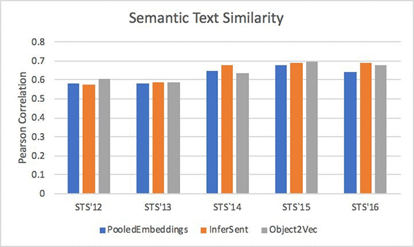
Despite being a general-purpose embedding algorithm for a range of input types, Amazon SageMaker Object2Vec has comparable performance results against some of the purpose-built embedding algorithms. See the following for the Pearson Correlation comparisons using various versions of the Semantic Text Similarity (STS) dataset, where we compare Object2Vec with a state-of-the-art model called InferSent.
Use cases for Object2Vec
We currently support learning embeddings of pairs of tokens, pairs of sequences, and pairs of token and sequence. There are many use cases that can be mapped into one of these representations. Next, we will take a look at three specific use cases:
- Collaborative recommendation system
- Multi-label document classification
- Sentence embeddings
Training with pairs of tokens: Collaborative recommendation system
Collaborative filtering is a popular technique for building recommendation systems. The main concept behind collaborative filtering is that users with similar tastes (based on observed user-item interactions) are more likely to have similar interactions with new items. Object2Vec can make recommendations by approximating the observed user-item interactions using low dimensional representations of users and items.
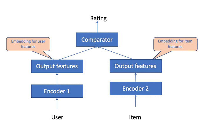
The following diagram shows how user-item interaction data can be used to learn the embedding of users and items. The resulting model can be used to predict user rating on a new item.
To see how SageMaker Object2Vec can be used for building a collaborative recommendation model, let’s take a look at this notebook. More specifically, we will show how to solve the following two different kinds of machine learning tasks using the MovieLens dataset.
- Task 1: Rating prediction as a regression problem
- Task 2: Movie recommendation as a classification problem
The MovieLens dataset contains paired data of (user,movie) and the corresponding ratings. The integer-id corresponding to a user is fed into one arm of Object2Vec and the integer-id corresponding to the movie is fed into the other arm. We use separate embedding-based encoders for users and movies to convert them into dense embeddings, which are passed into the comparator that makes prediction of the rating for a given (user, movie) pair. We will first show how to learn the embeddings of users and movies based on labeled training data. Then, we will demonstrate how to use the learned embeddings to make predictions of ratings on the held-out test set, and show that our model achieves accuracy comparable to some of the best tools available in the open source domain. See the following diagram for a high-level logic flow of the data processing and training pipeline.

In the data processing and preparation step, we will create a training data file, a validation data file, and a test data file, and the files will be copied to an Amazon S3 bucket. Amazon SageMaker Object2Vec takes input in JSON-lines format, so the raw MovieLens data will be converted to the format similar to the sample that follows. In this sample, in0 represents the user id, in1 represents the movie id, and the label represents the movie rating by the user for the movie. We will use the raw dataset to create a training dataset, a validation dataset, and a test dataset. During training time, the in0 value will be fed into one arm of the Object2Vec algorithm, and in1 will be fed into another arm.
{"in0": [1], "in1": [20], "label": 4.0}
{"in0": [1], "in1": [33], "label": 4.0}
{"in0": [1], "in1": [61], "label": 4.0}
{"in0": [1], "in1": [117], "label": 3.0}
{"in0": [1], "in1": [155], "label": 2.0}
For the training step, we will configure the necessary hyperparameters for task 1 and task 2. For task1, which is a regression job, we will set the “output_layer” hyperparameter to “mean_squared_error“, and for task 2, we will use “softmax” for the “output_layer”. Since the inputs are individual tokens, we set the network for both encoders to “pooled_embedding”.
Amazon SageMaker provides a Python SDK for easier integration with the SageMaker backend operations such as training and deployment. Here, we will use the Amazon SageMaker Estimator to kick off the training job. See the following code sample for the syntax in the Amazon SageMaker Python SDK for kicking off the rating prediction (regression) job.
regressor = sagemaker.estimator.Estimator(container,
                                          role,
                                          train_instance_count=1,
                                          train_instance_type='ml.p2.xlarge',
                                          output_path=output_path,
                                          sagemaker_session=sess)

## train, tune, and test the model
regressor.fit({'train': s3_train, 'validation':s3_valid, 'test':s3_test})
See the following for the code sample for kicking off a recommendation (classification) job.
classifier = sagemaker.estimator.Estimator(container,
                                    role,
                                    train_instance_count=1,
                                    train_instance_type='ml.p2.xlarge',
                                    output_path=output_path,
                                    sagemaker_session=sess)

## train, tune, and test the model
classifier.fit({'train': s3_train_c, 'validation':s3_valid_c, 'test':s3_test_c})
When the training job runs, it will output the following training and validation metrics in Amazon CloudWatch Logs and in the Jupyter notebook console.
[10/18/2018 14:39:43 INFO 140224059168576] Epoch 6 Training metrics:   mean_squared_error: 0.084 mean_absolute_error: 0.224
[10/18/2018 14:39:43 INFO 140224059168576] #quality_metric: host=algo-1, epoch=6, train mean_squared_error <loss>=0.084217468395
[10/18/2018 14:39:43 INFO 140224059168576] Epoch 6 Validation metrics: mean_squared_error: 0.931 mean_absolute_error: 0.762
[10/18/2018 14:39:43 INFO 140224059168576] #quality_metric: host=algo-1, epoch=6, validation mean_squared_error <loss>=0.930595424127
Check out the full notebook for detailed instructions.
Training with pairs of (one-hot vectors and sequences of one-hot vectors): Multi-label document classification
Document classification and tagging are common business challenges for many organizations, especially in the era of big data. There are unsupervised machine learning approaches such as topic modeling and supervised machine learning approaches such as multi-label classification. Object2Vec’s ability to support token and a sequence pair input is well suited for the multi-label document classification problem. See the following diagram on how document and label data can be fed into Object2Vec for multi-label classification training.
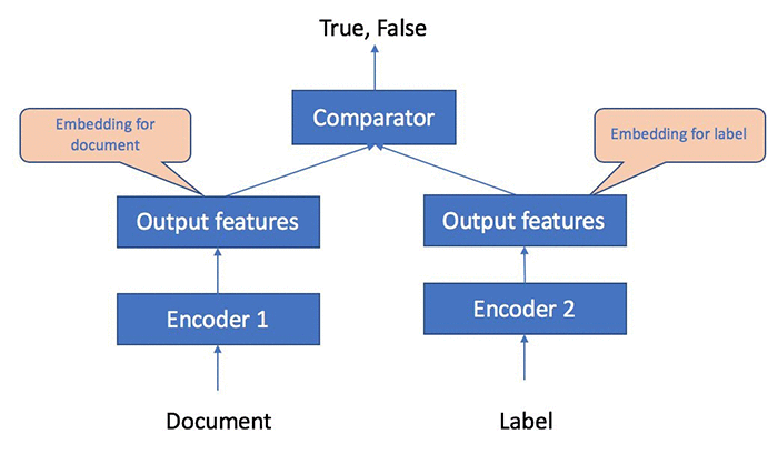
In this notebook example, we will show how to train Object2Vec on token, sequence pairs. The specific use case we consider is multi-labeled document classification. To model this problem, one arm of our architecture accepts a document represented as a sequence of word-ids as input. The other arm accepts the categorical label of the document represented as an integer-id as input. We convert multi-labeled documents into document, label pairs where each document is repeatedly paired with every label in the corpus. We apply a `positive’ relationship to a (document, label) pair if the document is tagged with the specific label in the ground truth data. Otherwise, the relationship between the document, label pair is marked as `negative.’ The encoder for the document arm would be a CNN or a BiLSTM which would convert the variable-length sequence into a fixed-length embedding. The encoder for the label arm would be a simple embedding encoder which would convert the label-id into dense embedding. These two would be passed to a comparator, which would emit scores that correspond to the model’s confidence in the two relationship types between the document and the label.
At training time, we associate all (document, label) pairs that exist in the training data with a “positive” relationship type, and we sample pairs with a “negative” relationship type from the cross-product of (documents, labels) such that the document is in the training data, but the pair (document, label) does not occur in the training data. If the same document has multiple labels, we generate a unique (document, label) pair with a “positive” relationship for each label that applies to the document. Such preprocessing is similar to how multi-labeled document classification is handled using multiple one-vs-rest classifiers.
At test time, given a document D, we pass the document to Object2Vec multiple times, where each time it is paired with one unique label L in the training set as input. We accept the label L as applicable to the document if the score for “positive” relationship type for the pair (D,L) is higher than a threshold.
Check out the full notebook for detailed instructions on running multi-label document classification with Object2Vec.
Training with pairs of (sequence of tokens, sequence of tokens): Sentence similarity
There are many practical use cases for sentence similarity. For example, in a customer support workflow, you might need to identify duplicate support tickets or route tickets to the correct support queue based on similarity of the text found in the ticket. Another example where sentence/text similarity can be used is information retrieval where a system can return a list of similar text given an input text.
Modeling sequences of tokens as embeddings is also relevant in contexts other than natural language. For example, a customer’s preferences can be modeled by the sequence of product-ids that he/she has bought in the recent past. We can learn a customer’s embedding by pairing sequences of product-ids bought by the customer as positive pairs and sequences of product-ids bought by different customers as negative examples. The embeddings thus learned can be used to find similar customers or can be used as features in a downstream supervised task.
In this notebook, we will demonstrate how to use Object2Vec to generate embeddings for sentences so they can be used for sentence similarity comparison. The following diagram shows the sentence pairs will be fed into the Object2Vec to learn the embeddings.
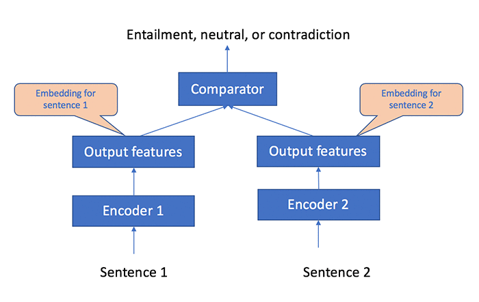
The high-level logical flow of the data processing and training pipeline is depicted in the following diagram.
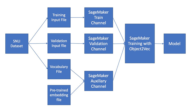
For training data, we will use The Stanford Natural Language Inference (SNLI) dataset, which consists of pairs of sentences labeled “entailment,” “neutral,” or “contradiction.” After the model is trained, we can use the trained model to convert any English sentences into fixed-length embeddings. We will measure the quality of the model by using a hold-out test dataset from the SNLI dataset. In the notebook, we will also measure the quality of embeddings on new sentences, by comparing the similarity of sentence pairs in the embedding space from the Semantic Text Similarity (STS) dataset and evaluate that against the human-labeled ground truth.
We will preprocess the SNLI data into a JSON line structure shown by the following sample data, so it can be consumed by the Object2Vec algorithm. In this sample, in0 and in1 represent two sentences respectively with the integers representing the words in the sentences, and the label representing the relationship (entailment, neutral, or contradiction) between the two sentences.
{"in0": [8976, 43036, 10889, 19131, 42641, 23620, 40005, 21984, 29937, 58],
"in1": [8653, 36222, 10889, 23971, 22084, 42641, 23620, 40005, 21984],
"label": 1}
Training this sentence similarity model is just like training any other models using the Amazon SageMaker built-in algorithms. You would first define data channels which include channels for training data, validation data, and auxiliary data which is for the vocabulary file and the pre-trained embedding file. You would then configure the necessary training hyperparameters and use an Amazon SageMaker estimator to kick off a training job. See the following sample code snippet on the syntax for using the Amazon SageMaker Estimator to start the training job.
regressor = sagemaker.estimator.Estimator(container,
                                          role,
                                          train_instance_count=1,
                                          train_instance_type='ml.p2.xlarge',
                                          output_path=output_path,
                                          sagemaker_session=sess)

regressor.fit(input_channels)
When the training job runs, you will see the following performance metrics being reported in Amazon CloudWatch Logs and directly inside the Jupyter notebook console after each epoch runs.
[10/14/2018 22:13:39 INFO 140406399915840] Completed Epoch: 0, time taken: 0:00:18.556232
[10/14/2018 22:13:39 INFO 140406399915840] Epoch 0 Training metrics:   perplexity: 2.433 cross_entropy: 0.889 accuracy: 0.582
[10/14/2018 22:13:39 INFO 140406399915840] #quality_metric: host=algo-1, epoch=0, train cross_entropy <loss>=0.88893990372
[10/14/2018 22:13:39 INFO 140406399915840] #quality_metric: host=algo-1, epoch=0, train accuracy <score>=0.582158705767
[10/14/2018 22:13:39 INFO 140406399915840] Epoch 0 Validation metrics: perplexity: 2.139 cross_entropy: 0.760 accuracy: 0.669
[10/14/2018 22:13:39 INFO 140406399915840] #quality_metric: host=algo-1, epoch=0, validation cross_entropy <loss>=0.760480128229
[10/14/2018 22:13:39 INFO 140406399915840] #quality_metric: host=algo-1, epoch=0, validation accuracy <score>=0.668823242188
Check out the full notebook for detailed instructions on running the embedding pipeline and additional code samples on how to use the STS dataset for measuring sentence similarity.
Conclusion
In this blog post, we introduced to you the new Amazon SageMaker Object2Vec algorithm. This post and the companion notebooks show you how Object2Vec works and how it can be applied to a range of practical business use cases.
About the authors
 David Ping is a Principal Solutions Architect with the AWS Solutions Architecture organization. He works with our customers to build cloud and machine learning solutions using AWS. He lives in the NY metro area and enjoys learning the latest machine learning technologies.
 Patrick Ng is a Software Development Engineer in the Verticals and Applications Group at AWS AI. He works on building scalable distributed machine learning algorithms, with focus in the area of deep neural networks and natural language processing. Before Amazon, he obtained his PhD in Computer Science from the Cornell University and worked at startup companies building machine learning systems.
 Cheng Tang is an Applied Scientist in the Verticals and Applications Group at AWS AI. Broadly interested in machine learning research and its applications to the natural language processing domain, Cheng finds great inspiration to be part of both research and industrialization of machine learning/deep learning algorithms, and she is thrilled to see them delivered to the customers.
 Saswata Chakravarty is a Software Engineer in the AWS Algorithms team. He works on bringing fast and scalable algorithms to Amazon SageMaker and making them easy to use for customers.
 Ramesh Nallapati is a Senior Applied Scientist in the Verticals and Applications Group at AWS AI. He works on building novel deep neural networks at scale primarily in the natural language processing domain. He is very passionate about deep learning, and enjoys learning about latest developments in AI and is excited about contributing to this field to the best of his abilities.
 Bing Xiang is a Principal Scientist and Head of Verticals and Applications Group at AWS AI. He leads a team of scientists and engineers working on deep learning, machine learning, and natural language processing for multiple AWS services.
Acknowledgments
We would like to thank Orchid Majumder, Software Development Engineer, AI Platforms team, for his early contributions on this project, as well as Laurence Rouesnel, Group Manager for the Algorithms & Platforms Group in Amazon AI Labs, and Leo Dirac, Senior Principal Engineer, AI Platforms team, for their expert advice and guidance throughout this work.

 Paul Zhao is a Sr. Product Manager at AWS Machine Learning. He manages the Amazon Transcribe service. Outside of work, Paul is a motorcycle enthusiast and avid woodworker.
 Paul Kohan is a Sr. Software Engineer at Amazon Transcribe. Outside of work Paul enjoys hanging out with his dog, Toby, and playing video and board games.


 Sifei Li is a Software Engineer in Amazon AI where she’s working on building Amazon Machine Learning Platforms and was part of the launch team for Amazon SageMaker.
 Sumit Thakur is a Senior Product Manager for AWS Machine Learning Platforms where he loves working on products that make it easy for customers to get started with machine learning on cloud. He is product manager for Amazon SageMaker and AWS Deep Learning AMI. In his spare time, he likes connecting with nature and watching sci-fi TV series.


 Jared Katzman is a Software Engineer in the AWS AI Labs organization. They are interested in researching ways we can use machine learning and technology for social good. In their spare time, they run a mentorship program for LGBTQ+ students interested in technology.
 Baris Coskun is a Senior Applied Scientist in the AWS External Security Services, where he leads a team of scientists working on machine learning and information security.
 The Kinesis Video Streams client library enables scalable, a- least-once-processing of the media across a distributed set of workers, manages the reliable invocation of Amazon SageMaker endpoints, and publishing of inference results into a Kinesis data stream for subsequent processing. Specifically, the library determines the Kinesis Video streams that have to be processed, connects to the streams, and refreshes them periodically to include/ exclude streams for processing. The software instantiates a worker that runs consumers which are responsible for processing a Kinesis Video stream at any given time. As part of this, it also maintains leases for every consumer running in (and across) workers to coordinate among themselves the ability to process the various streams. It also ensures reliable, at-least-once-processing of the media fragments by managing checkpoints on a per lease-stream basis.
 The AWS CloudFormation template automates the deployment of all relevant AWS infrastructure in the customer’s own account, to read media from Kinesis Video Streams and invoke the Amazon SageMaker endpoint for ML-based analytics. This saves time to build, operate, and scale the integrated capability.




 Aditya Krishnan is the head of Amazon Kinesis Video Streams. In this role he has the good fortune of working with customers, hardware and software partners, and a phenomenal engineering team to deliver on the vision of making it ridiculously easy to stream video from internet-enabled camera devices at massive scale.
 Jagadeesh Pusapadi is a Solutions Architect with AWS working with customers on their strategic initiatives. He helps customers build innovative solutions on AWS Cloud by providing architectural guidance to achieve desired business outcomes.


 Patricia Grao is a Software Development Manager in Amazon AI. She became passionate about machine learning while working in search ranking and query understanding in Amazon Search. She was part of the team that launched Amazon SageMaker Automatic Model Tuning.
 Fela Winkelmolen works as an applied scientists for Amazon AI and was part of the team that launched the Automatic Model Tuning feature of Amazon SageMaker
 Fan Li is a Product Manager of Amazon SageMaker. He used to be a big fan of ballroom dance but now loves whatever his 8-year-old son likes.
 When it comes to understanding unstructured text in a specific domain, natural language doesn’t come much more specialized than in the legal profession. The “legalese” used in most legal documents is famous for its complex syntax, nomenclature and structure. It’s a great example of where Comprehend Custom Entitites can help; we worked with LexisNexis while developing these new capabilities, to extract legal entities from hundreds of millions of documents, with very high accuracy.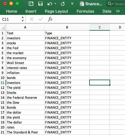
 Nino Bice is a Sr. Product Manager leading product for Amazon Comprehend, AWS’s natural language processing service.
 Robin Dautricourt is a Principle Product Manager for Amazon Text-to-Speech, and he leads product management for Amazon Polly. He enjoys innovating on behalf of customers, to launch features that will benefit their business needs and end users. He enjoys spending his free time with his wife and kids.