Unsupervised Anomaly Detection for Univariate & Multivariate Data.

Anomaly detection is the process of identifying unexpected items or events in data sets, which differ from the norm. And anomaly detection is often applied on unlabeled data which is known as unsupervised anomaly detection. Anomaly detection has two basic assumptions:

• Anomalies only occur very rarely in the data.
• Their features differ from the normal instances significantly.

Univariate Anomaly Detection

Before we get to Multivariate anomaly detection, I think its necessary to work through a simple example of Univariate anomaly detection method in which we detect outliers from a distribution of values in a single feature space.

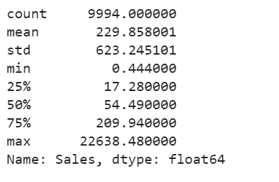
We are using the Super Store Sales data set that can be downloaded from here, and we are going to find patterns in Sales and Profit separately that do not conform to expected behavior. That is, spotting outliers for one variable at a time.

import pandas as pd
import numpy as np
import matplotlib.pyplot as plt
import seaborn as sns
import matplotlib
from sklearn.ensemble import IsolationForest

Distribution of the Sales

df = pd.read_excel("Superstore.xls")
df['Sales'].describe()

plt.scatter(range(df.shape[0]), np.sort(df['Sales'].values))
plt.xlabel('index')
plt.ylabel('Sales')
plt.title("Sales distribution")
sns.despine()

sns.distplot(df['Sales'])
plt.title("Distribution of Sales")
sns.despine()

print("Skewness: %f" % df['Sales'].skew())
print("Kurtosis: %f" % df['Sales'].kurt())

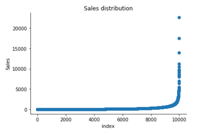
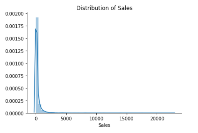
The Superstore’s sales distribution is far from a normal distribution, and it has a positive long thin tail, the mass of the distribution is concentrated on the left of the figure. And the tail sales distribution far exceeds the tails of the normal distribution.

There are one region where the data has low probability to appear which is on the right side of the distribution.

Distribution of the Profit

df['Profit'].describe()

plt.scatter(range(df.shape[0]), np.sort(df['Profit'].values))
plt.xlabel('index')
plt.ylabel('Profit')
plt.title("Profit distribution")
sns.despine()

sns.distplot(df['Profit'])
plt.title("Distribution of Profit")
sns.despine()

print("Skewness: %f" % df['Profit'].skew())
print("Kurtosis: %f" % df['Profit'].kurt())

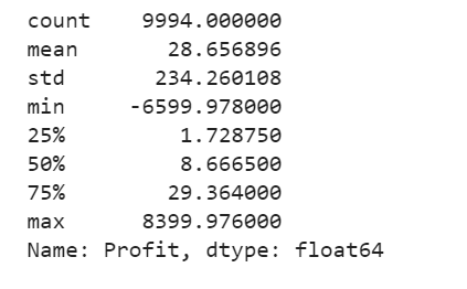
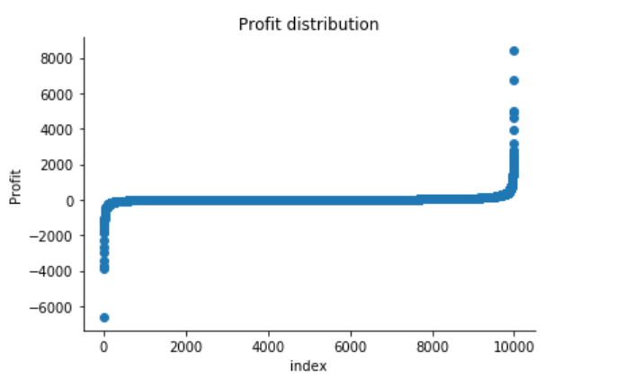
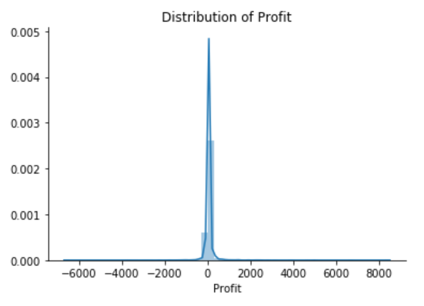
The Superstore’s Profit distribution has both a positive tail and negative tail. However, the positive tail is longer than the negative tail. So the distribution is positive skewed, and the data are heavy-tailed or profusion of outliers.

There are two regions where the data has low probability to appear: one on the right side of the distribution, another one on the left.

Univariate Anomaly Detection on Sales

Isolation Forest is an algorithm to detect outliers that returns the anomaly score of each sample using the IsolationForest algorithm which is based on the fact that anomalies are data points that are few and different. Isolation Forest is a tree-based model. In these trees, partitions are created by first randomly selecting a feature and then selecting a random split value between the minimum and maximum value of the selected feature.

The following process shows how IsolationForest behaves in the case of the Susperstore’s sales, and the algorithm was implemented in Sklearn and the code was largely borrowed from this tutorial

• Trained IsolationForest using the Sales data.
• Store the Sales in the NumPy array for using in our models later.
• Computed the anomaly score for each observation. The anomaly score of an input sample is computed as the mean anomaly score of the trees in the forest.
• Classified each observation as an outlier or non-outlier.
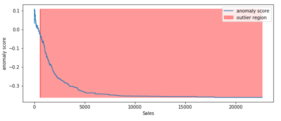
• The visualization highlights the regions where the outliers fall.

According to the above results and visualization, It seems that Sales that exceeds 1000 would be definitely considered as an outlier.

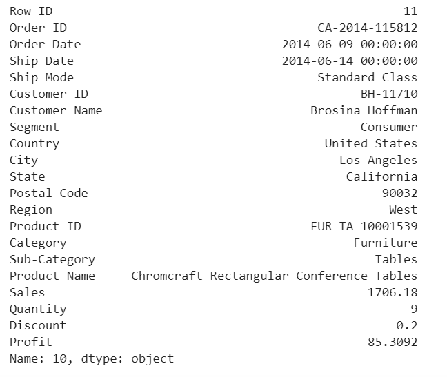
Visually investigate one anomaly

df.iloc[10]

This purchase seems normal to me expect it was a larger amount of sales compared with the other orders in the data.

Univariate Anomaly Detection on Profit

• Trained IsolationForest using the Profit variable.
• Store the Profit in the NumPy array for using in our models later.
• Computed the anomaly score for each observation. The anomaly score of an input sample is computed as the mean anomaly score of the trees in the forest.
• Classified each observation as an outlier or non-outlier.
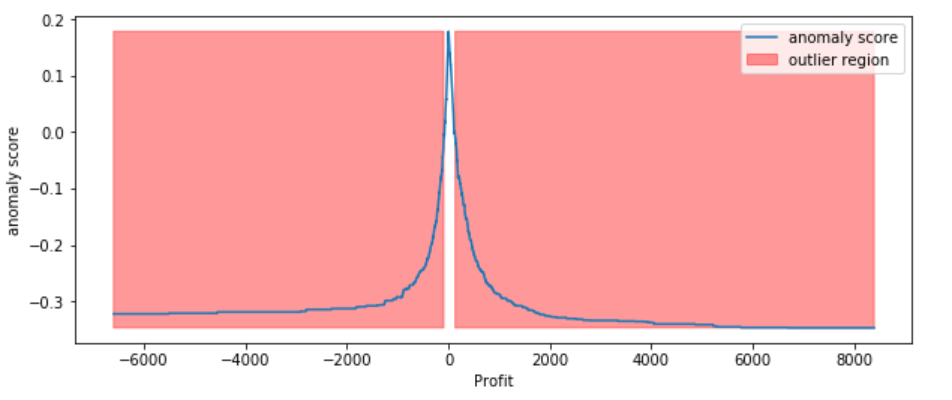
• The visualization highlights the regions where the outliers fall.

Visually investigate some of the anomalies

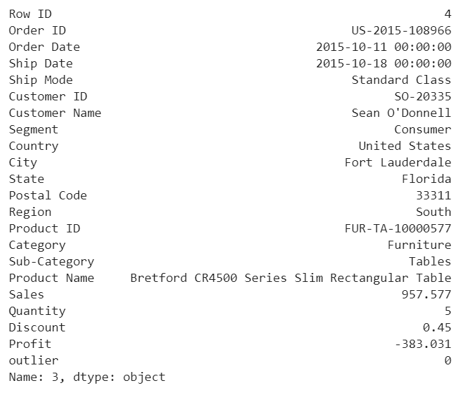
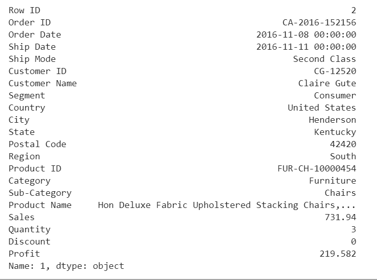
According to the above results and visualization, It seems that Profit that below -100 or exceeds 100 would be considered as an outlier, let’s visually examine one example each that determined by our model and to see whether they make sense.

df.iloc[3]

Any negative profit would be an anomaly and should be further investigate, this goes without saying

df.iloc[1]

Our model determined that this order with a large profit is an anomaly. However, when we investigate this order, it could be just a product that has a relatively high margin.

The above two visualizations show the anomaly scores and highlighted the regions where the outliers are. As expected, the anomaly score reflects the shape of the underlying distribution and the outlier regions correspond to low probability areas.

However, Univariate analysis can only get us thus far. We may realize that some of these anomalies that determined by our models are not the anomalies we expected. When our data is multidimensional as opposed to univariate, the approaches to anomaly detection become more computationally intensive and more mathematically complex.

Multivariate Anomaly Detection

Most of the analysis that we end up doing are multivariate due to complexity of the world we are living in. In multivariate anomaly detection, outlier is a combined unusual score on at least two variables.

So, using the Sales and Profit variables, we are going to build an unsupervised multivariate anomaly detection method based on several models.

We are using PyOD which is a Python library for detecting anomalies in multivariate data. The library was developed by Yue Zhao.

Sales & Profit

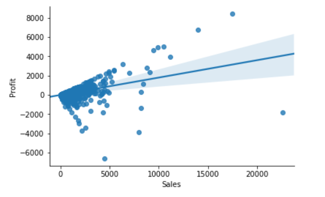
When we are in business, we expect that Sales & Profit are positive correlated. If some of the Sales data points and Profit data points are not positive correlated, they would be considered as outliers and need to be further investigated.

sns.regplot(x="Sales", y="Profit", data=df)
sns.despine();

From the above correlation chart, we can see that some of the data points are obvious outliers such as extreme low and extreme high values.

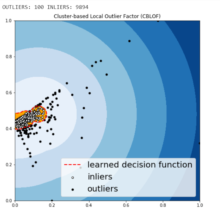
Cluster-based Local Outlier Factor (CBLOF)

The CBLOF calculates the outlier score based on cluster-based local outlier factor. An anomaly score is computed by the distance of each instance to its cluster center multiplied by the instances belonging to its cluster. PyOD library includes the CBLOF implementation.

The following code are borrowed from PyOD tutorial combined with this article.

• Scaling Sales and Profit to between zero and one.
• Arbitrarily set outliers fraction as 1% based on trial and best guess.
• Fit the data to the CBLOF model and predict the results.
• Use threshold value to consider a data point is inlier or outlier.
• Use decision function to calculate the anomaly score for every point.

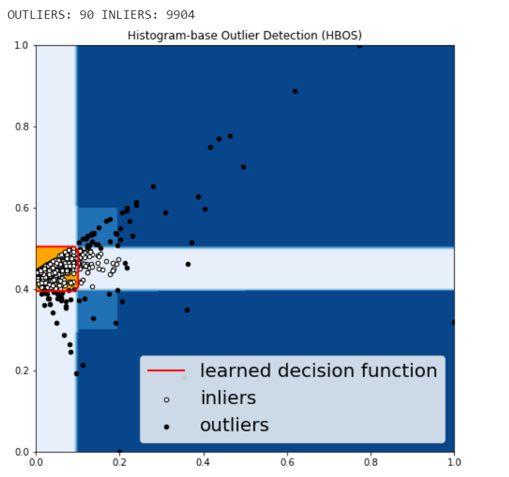
Histogram-based Outlier Detection (HBOS)

HBOS assumes the feature independence and calculates the degree of anomalies by building histograms. In multivariate anomaly detection, a histogram for each single feature can be computed, scored individually and combined at the end. When using PyOD library, the code are very similar with the CBLOF.

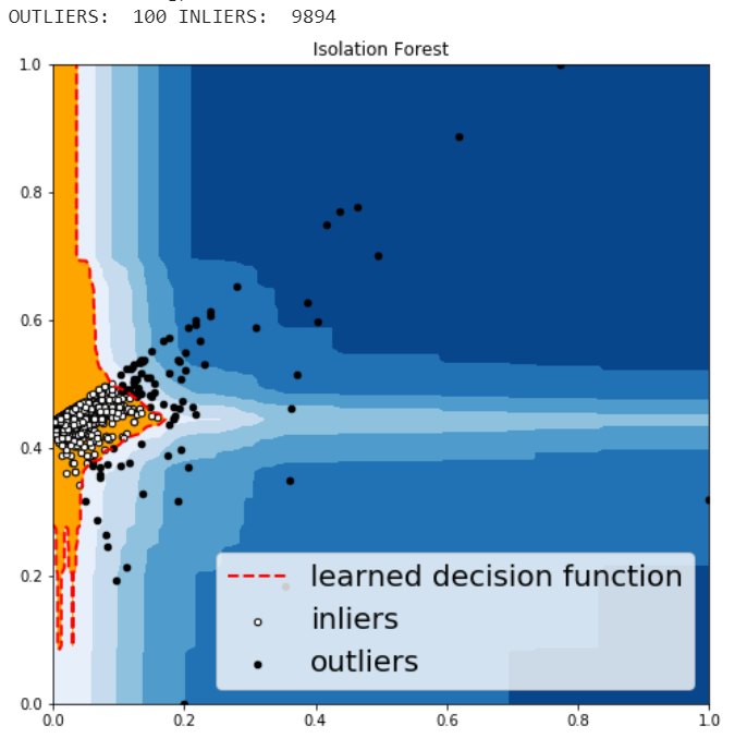
Isolation Forest

Isolation Forest is similar in principle to Random Forest and is built on the basis of decision trees. Isolation Forest isolates observations by randomly selecting a feature and then randomly selecting a split value between the maximum and minimum values of that selected feature.

The PyOD Isolation Forest module is a wrapper of Scikit-learn Isolation Forest with more functionalities.

K – Nearest Neighbors (KNN)

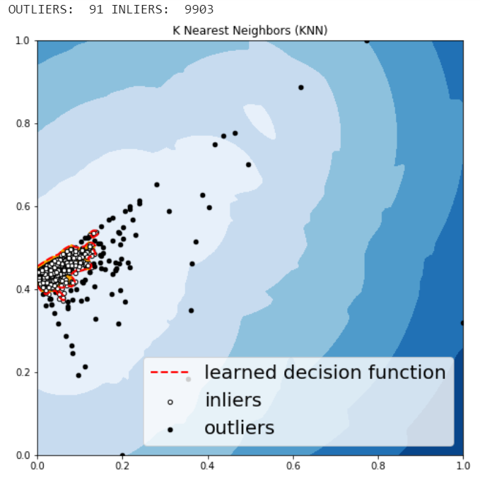
KNN is one of the simplest methods in anomaly detection. For a data point, its distance to its kth nearest neighbor could be viewed as the outlier score.

The anomalies predicted by the above four algorithms were not very different.

Visually investigate some of the anomalies

We may want to investigate each of the outliers that determined by our model, for example, let’s look in details for a couple of outliers that determined by KNN, and try to understand what make them anomalies.

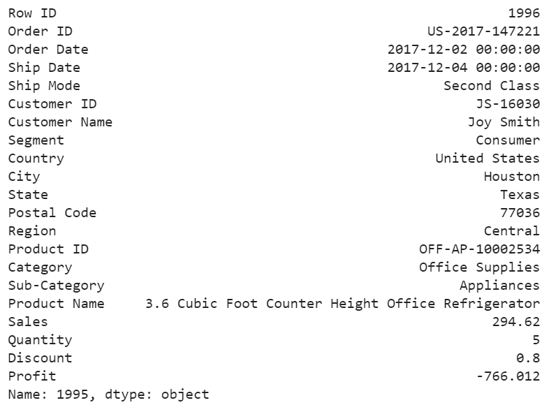
df.iloc[1995]

For this particular order, a customer purchased 5 products with total price at 294.62 and profit at lower than -766, with 80% discount. It seems like a clearance. We should be aware of the loss for each product we sell.

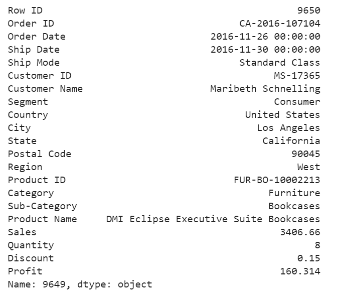
df.iloc[9649]

For this purchase, it seems to me that the profit at around 4.7% is too small and the model determined that this order is an anomaly.

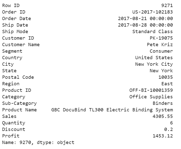
df.iloc[9270]

For the above order, a customer purchased 6 product at 4305 in total price, after 20% discount, we still get over 33% of the profit. We would love to have more of these kind of anomalies.

Jupyter notebook for the above analysis can be found on Github. Enjoy the rest of the week.

Anomaly Detection for Dummies was originally published in Towards Data Science on Medium, where people are continuing the conversation by highlighting and responding to this story.