[D] Why We Open Sourced GROVER
Rowan Zellers writes https://thegradient.pub/why-we-released-grover/
submitted by /u/hughbzhang
[link] [comments]
Rowan Zellers writes https://thegradient.pub/why-we-released-grover/
submitted by /u/hughbzhang
[link] [comments]
In this post, we will explore using Bayesian Logistic Regression in order to predict whether or not a customer will subscribe a term deposit after the marketing campaign the bank performed.
We want to be able to accomplish:
I am sure you are familiar with the dataset. We built a logistic regression model using standard machine learning methods with this dataset a while ago. And today we are going to apply Bayesian methods to fit a logistic regression model and then interpret the resulting model parameters. Let’s get started!
The goal of this dataset is to create a binary classification model that predicts whether or not a customer will subscribe a term deposit after a marketing campaign the bank performed, based on many indicators. The target variable is given as y and takes on a value of 1 if the customer has subscribed and 0 otherwise.
This is an imbalanced class problem because there are significantly more customers did not subscribe the term deposit than the ones did.
import pandas as pd
import numpy as np
import seaborn as sns
import matplotlib.pyplot as plt
import pymc3 as pm
import arviz as az
import matplotlib.lines as mlines
import warnings
warnings.filterwarnings('ignore')
from collections import OrderedDict
import theano
import theano.tensor as tt
import itertools
from IPython.core.pylabtools import figsize
pd.set_option('display.max_columns', 30)
from sklearn.metrics import accuracy_score, f1_score, confusion_matrix
df = pd.read_csv('banking.csv')
As part of EDA, we will plot a few visualizations.
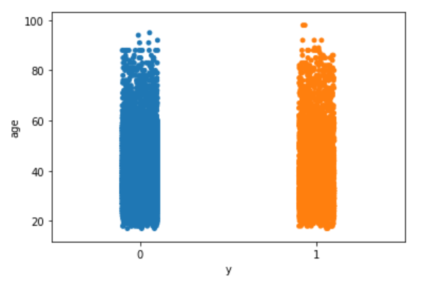
sns.stripplot(x="y", y="age", data=df, jitter=True)
plt.show();
sns.stripplot(x="y", y="euribor3m", data=df, jitter=True)
plt.show();
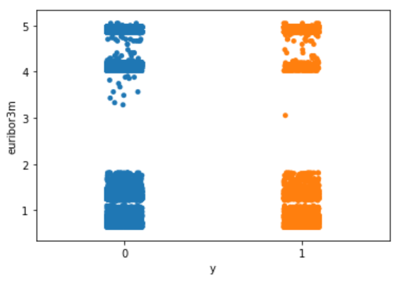
Nothing particularly interesting here.
The following is my way of making all of the variables numeric. You may have a better way of doing it.
We are going to begin with the simplest possible logistic model, using just one independent variable or feature, the duration.
outcome = df['y']
data = df[['age', 'job', 'marital', 'education', 'default', 'housing', 'loan', 'contact', 'month', 'day_of_week', 'duration', 'campaign', 'pdays', 'previous', 'poutcome', 'euribor3m']]
data['outcome'] = outcome
data.corr()['outcome'].sort_values(ascending=False)
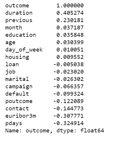
With the data in the right format, we can start building our first and simplest logistic model with PyMC3:
We are going to plot the fitted sigmoid curve and the decision boundary:
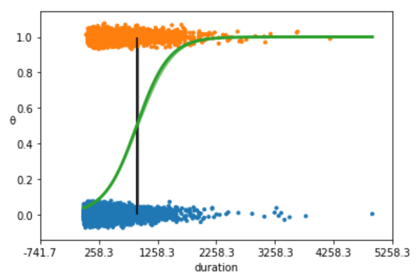
We summarize the inferred parameters values for easier analysis of the results and check how well the model did:
az.summary(trace_simple, var_names=['α', 'β'])

As you can see, the values of α and β are very narrowed defined. This is totally reasonable, given that we are fitting a binary fitted line to a perfectly aligned set of points.
Let’s run a posterior predictive check to explore how well our model captures the data. We can let PyMC3 do the hard work of sampling from the posterior for us:
ppc = pm.sample_ppc(trace_simple, model=model_simple, samples=500)
preds = np.rint(ppc['y_1'].mean(axis=0)).astype('int')
print('Accuracy of the simplest model:', accuracy_score(preds, data['outcome']))
print('f1 score of the simplest model:', f1_score(preds, data['outcome']))

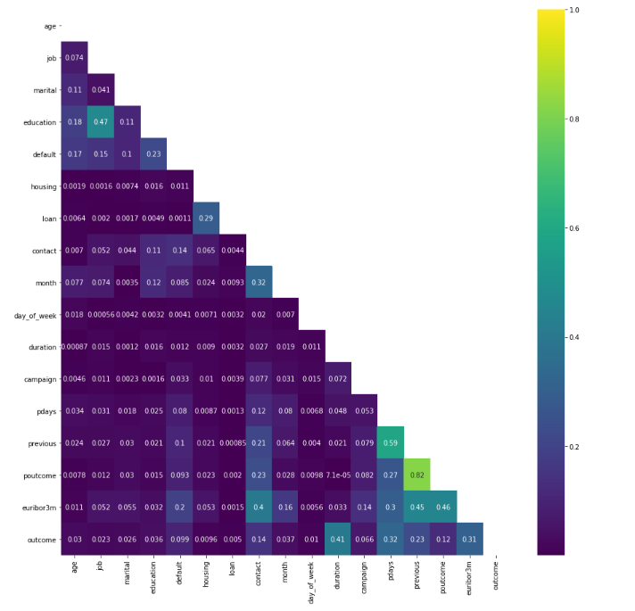
We plot a heat map to show the correlations between each variables.
plt.figure(figsize=(15, 15))
corr = data.corr()
mask = np.tri(*corr.shape).T
sns.heatmap(corr.abs(), mask=mask, annot=True, cmap='viridis');
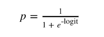
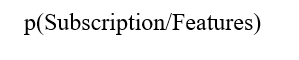
logit = β0 + β1(age) + β2(age)2 + β3(job) + β4(marital) + β5(education) + β6(default) + β7(housing) + β8(loan) + β9(contact) + β10(month) + β11(day_of_week) + β12(duration) + β13(campaign) + β14(campaign) + β15(pdays) + β16(previous) + β17(poutcome) + β18(euribor3m) and y = 1 if outcome is yes and y = 0 otherwise.
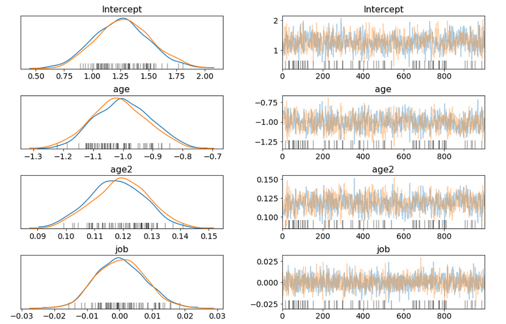
Above I only show part of the trace plot.
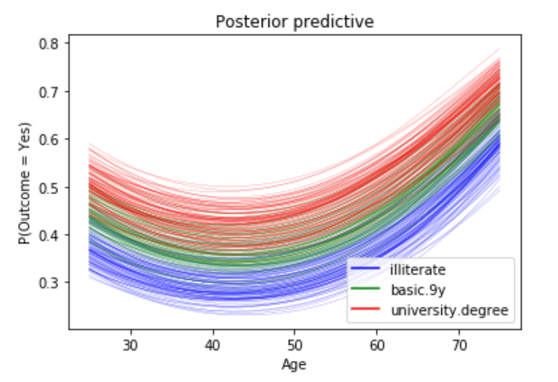
I want to be able to answer questions like:
b = trace['education']
plt.hist(np.exp(b), bins=20, normed=True)
plt.xlabel("Odds Ratio")
plt.show();
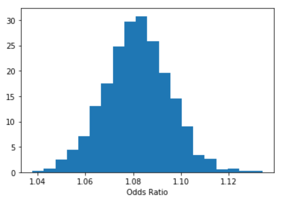
lb, ub = np.percentile(b, 2.5), np.percentile(b, 97.5)
print("P(%.3f < Odds Ratio < %.3f) = 0.95" % (np.exp(lb), np.exp(ub)))

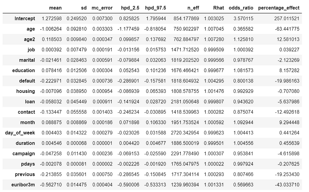
stat_df = pm.summary(trace)
stat_df['odds_ratio'] = np.exp(stat_df['mean'])
stat_df['percentage_effect'] = 100 * (stat_df['odds_ratio'] - 1)
stat_df
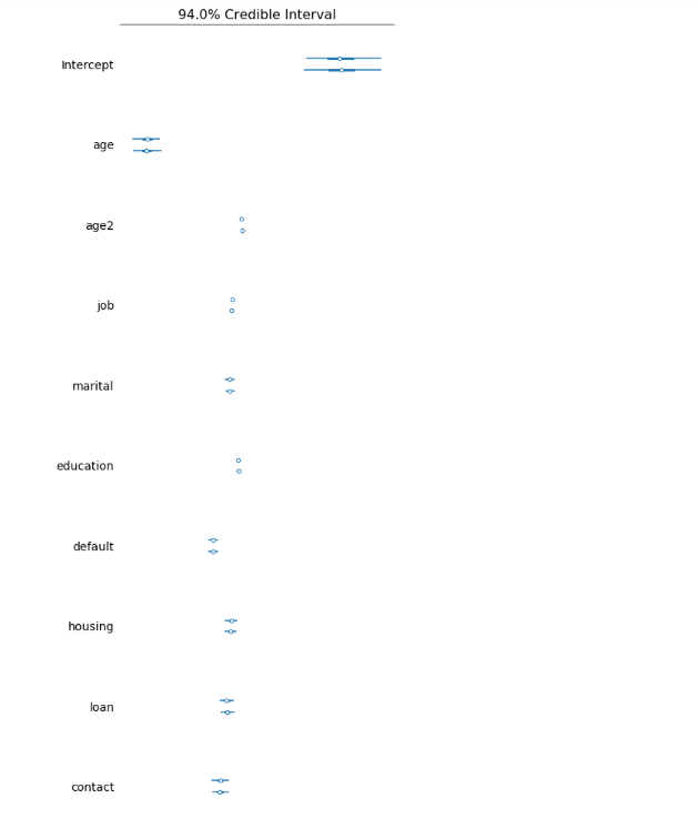
Its hard to show the entire forest plot, I only show part of it, but its enough for us to say that there’s a baseline probability of subscribing a term deposit. Beyond that, age has the biggest effect on subscribing, followed by contact.
model_trace_dict = dict()
for nm in ['k1', 'k2', 'k3']:
    models_lin[nm].name = nm
    model_trace_dict.update({models_lin[nm]: traces_lin[nm]})
dfwaic = pm.compare(model_trace_dict, ic='WAIC')
dfwaic
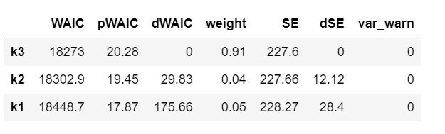
pm.compareplot(dfwaic);
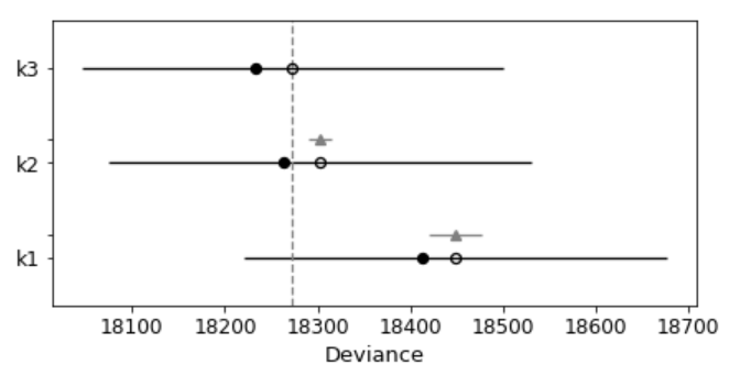
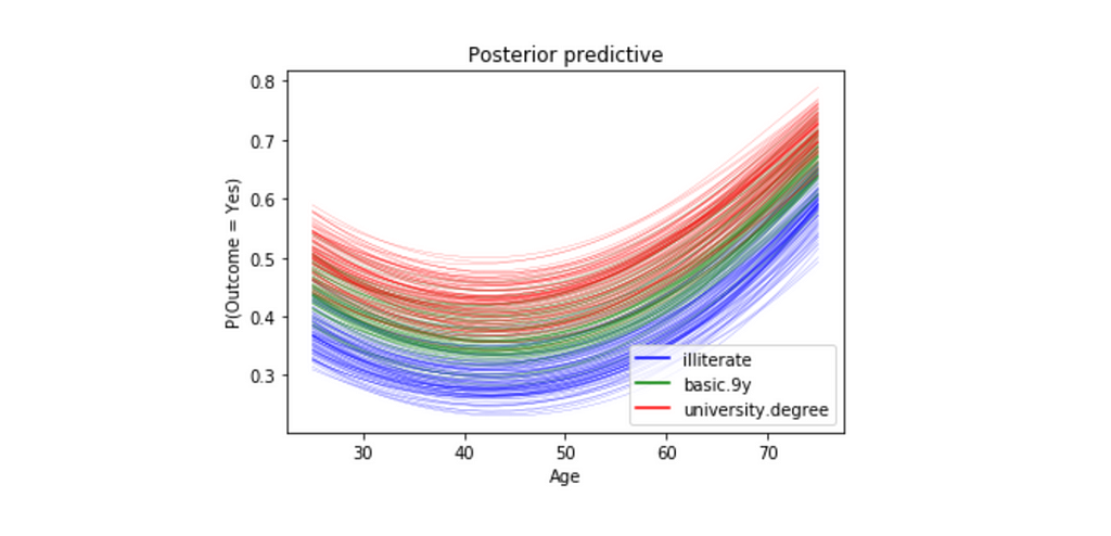
This confirms that the model that includes square of age is better than the model without.
Unlike standard machine learning, Bayesian focused on model interpretability around a prediction. But I’am curious to know what we will get if we calculate the standard machine learning metrics.
We are going to calculate the metrics using the mean value of the parameters as a “most likely” estimate.
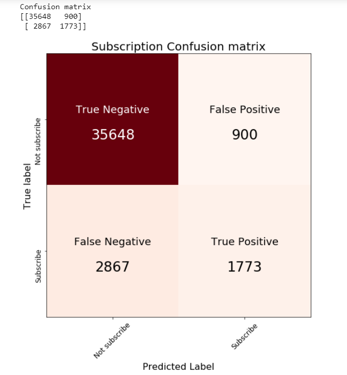
print('Accuracy of the full model: ', accuracy_score(preds, data['outcome']))
print('f1 score of the full model: ', f1_score(preds, data['outcome']))

Jupyter notebook can be found on Github. Have a great week!
References:
The book: Bayesian Analysis with Python, Second Edition
Building a Bayesian Logistic Regression with Python and PyMC3 was originally published in Towards Data Science on Medium, where people are continuing the conversation by highlighting and responding to this story.
The platform for Machine Learning methods dependencies 3D visualization is available now!
www.infornopolitan.xyz/backronym
At some moment I realized that my knowledge in ML is very limited, and ideas are poor. I know a couple of dozen models and this is a very small part of the total amount that can be very useful to me.
It seemed to me that if I will understand more models, my qualities as a researcher would certainly increase. This idea strongly motivated me to start meticulously studying articles from the conference.
I had no wish to represent dependencies as a table or a list, I wanted something more natural. A little thought, I realized that to have a strictly fixed graph, with edges between models and their components is interesting. Work in progress, but I believe, together we can do it much better!
submitted by /u/postmachines
[link] [comments]
Abstract:
A machine learning system can score well on a given test set by relying on heuristics that are effective for frequent example types but break down in more challenging cases. We study this issue within natural language inference (NLI), the task of determining whether one sentence entails another. We hypothesize that statistical NLI models may adopt three fallible syntactic heuristics: the lexical overlap heuristic, the subsequence heuristic, and the constituent heuristic. To determine whether models have adopted these heuristics, we introduce a controlled evaluation set called HANS (Heuristic Analysis for NLI Systems), which contains many examples where the heuristics fail. We find that models trained on MNLI, including BERT, a state-of-the-art model, perform very poorly on HANS, suggesting that they have indeed adopted these heuristics. We conclude that there is substantial room for improvement in NLI systems, and that the HANS dataset can motivate and measure progress in this area
Paper: https://arxiv.org/abs/1902.01007
Code for new dataset: https://github.com/tommccoy1/hans
submitted by /u/downtownslim
[link] [comments]
Hi everyone,
I am an academic researcher venturing into machine learning for one of my projects. I am trying to identify the gender of company executives based on their recorded voice over the phone. Here are the different datasets that I am working with:
I have tried a few different models on the training dataset, with great success. When I split the training dataset 80% 20% to run some tests, I get an accuracy of roughly 97%. When I apply the saved model to the testing dataset from the real population, accuracy drops to 85%. I am worried that this is in part due to the imbalance in gender.
What would be the best practices to tackle such problem?
Thanks a lot!
submitted by /u/newtomtl83
[link] [comments]
Microsoft press release: https://news.microsoft.com/2019/07/22/openai-forms-exclusive-computing-partnership-with-microsoft-to-build-new-azure-ai-supercomputing-technologies/
OpenAI press release: https://openai.com/blog/microsoft/
Microsoft is investing $1 billion in OpenAI to support us building artificial general intelligence (AGI) with widely distributed economic benefits. We’re partnering to develop a hardware and software platform within Microsoft Azure which will scale to AGI. We’ll jointly develop new Azure AI supercomputing technologies, and Microsoft will become our exclusive cloud provider—so we’ll be working hard together to further extend Microsoft Azure’s capabilities in large-scale AI systems.
submitted by /u/Reiinakano
[link] [comments]
![[R] Spectral Analysis of Latent Representations](https://a.thumbs.redditmedia.com/Lkk3LhBYs6RNLu9aBd4T1dktlW_vUweFM6Uwh52JoK4.jpg "[R] Spectral Analysis of Latent Representations") |
arXiv: https://arxiv.org/abs/1907.08589 PyTorch/Keras implementation: https://github.com/delve-team/delve Metric for analyzing deep neural network layers and fine-tuning architecture. Contributors to code/next paper are welcome! submitted by /u/justinshenk |
I need to learn a function that happens to have periodic components (along with non-periodic stuff) . I’d like to use only deep learning for reasons. Simple feed-forward networks suffer from this problem:
https://i.redd.it/6xfltw3xs6d21.png
Is there some standard way of doing so? It seems like sine activations are really hard to train, and the Fourier transform is afflicted with the curse of dimensionality, so learning on the frequency domain is not going to work either. Thanks in advance!
submitted by /u/mlboi
[link] [comments]