Building a Bayesian Logistic Regression with Python and PyMC3
How likely am I to subscribe a term deposit? Posterior probability, credible interval, odds ratio, WAIC
In this post, we will explore using Bayesian Logistic Regression in order to predict whether or not a customer will subscribe a term deposit after the marketing campaign the bank performed.
We want to be able to accomplish:
- How likely a customer to subscribe a term deposit?
- Experimenting of variables selection techniques.
- Explorations of the variables so serves as a good example of Exploratory Data Analysis and how that can guide the model creation and selection process.
I am sure you are familiar with the dataset. We built a logistic regression model using standard machine learning methods with this dataset a while ago. And today we are going to apply Bayesian methods to fit a logistic regression model and then interpret the resulting model parameters. Let’s get started!
The Data
The goal of this dataset is to create a binary classification model that predicts whether or not a customer will subscribe a term deposit after a marketing campaign the bank performed, based on many indicators. The target variable is given as y and takes on a value of 1 if the customer has subscribed and 0 otherwise.
This is an imbalanced class problem because there are significantly more customers did not subscribe the term deposit than the ones did.
import pandas as pd
import numpy as np
import seaborn as sns
import matplotlib.pyplot as plt
import pymc3 as pm
import arviz as az
import matplotlib.lines as mlines
import warnings
warnings.filterwarnings('ignore')
from collections import OrderedDict
import theano
import theano.tensor as tt
import itertools
from IPython.core.pylabtools import figsize
pd.set_option('display.max_columns', 30)
from sklearn.metrics import accuracy_score, f1_score, confusion_matrix
df = pd.read_csv('banking.csv')
As part of EDA, we will plot a few visualizations.
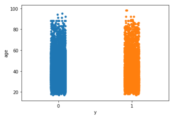
- Explore the target variable versus customers’ age using the stripplot function from seaborn:
sns.stripplot(x="y", y="age", data=df, jitter=True)
plt.show();
- Explore the target variable versus euribor3m using the stripplot function from seaborn:
sns.stripplot(x="y", y="euribor3m", data=df, jitter=True)
plt.show();
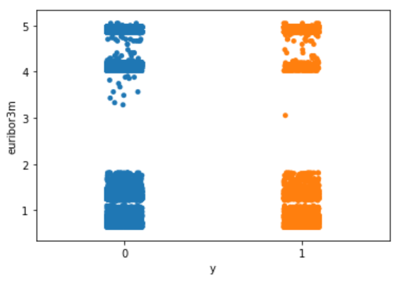
Nothing particularly interesting here.
The following is my way of making all of the variables numeric. You may have a better way of doing it.
Logistic Regression with One Independent Variable
We are going to begin with the simplest possible logistic model, using just one independent variable or feature, the duration.
outcome = df['y']
data = df[['age', 'job', 'marital', 'education', 'default', 'housing', 'loan', 'contact', 'month', 'day_of_week', 'duration', 'campaign', 'pdays', 'previous', 'poutcome', 'euribor3m']]
data['outcome'] = outcome
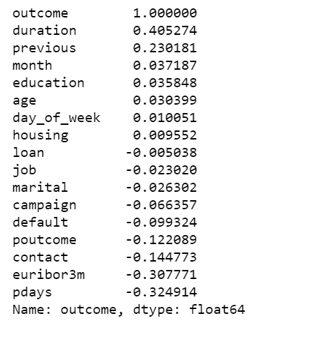
data.corr()['outcome'].sort_values(ascending=False)
With the data in the right format, we can start building our first and simplest logistic model with PyMC3:
- Centering the data can help with the sampling.
- One of the deterministic variables θ is the output of the logistic function applied to the μ variable.
- Another deterministic variables bd is the boundary function.
- pm.math.sigmoid is the Theano function with the same name.
We are going to plot the fitted sigmoid curve and the decision boundary:
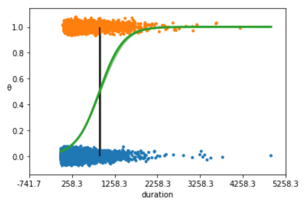
- The above plot shows non subscription vs. subscription (y = 0, y = 1).
- The S-shaped (green) line is the mean value of θ. This line can be interpreted as the probability of a subscription, given that we know that the last time contact duration(the value of the duration).
- The boundary decision is represented as a (black) vertical line. According to the boundary decision, the values of duration to the left correspond to y = 0 (non subscription), and the values to the right to y = 1 (subscription).
We summarize the inferred parameters values for easier analysis of the results and check how well the model did:
az.summary(trace_simple, var_names=['α', 'β'])
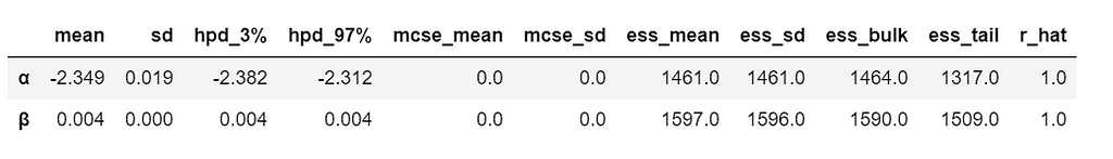
As you can see, the values of α and β are very narrowed defined. This is totally reasonable, given that we are fitting a binary fitted line to a perfectly aligned set of points.
Let’s run a posterior predictive check to explore how well our model captures the data. We can let PyMC3 do the hard work of sampling from the posterior for us:
ppc = pm.sample_ppc(trace_simple, model=model_simple, samples=500)
preds = np.rint(ppc['y_1'].mean(axis=0)).astype('int')
print('Accuracy of the simplest model:', accuracy_score(preds, data['outcome']))
print('f1 score of the simplest model:', f1_score(preds, data['outcome']))

Correlation of the Data
We plot a heat map to show the correlations between each variables.
plt.figure(figsize=(15, 15))
corr = data.corr()
mask = np.tri(*corr.shape).T
sns.heatmap(corr.abs(), mask=mask, annot=True, cmap='viridis');
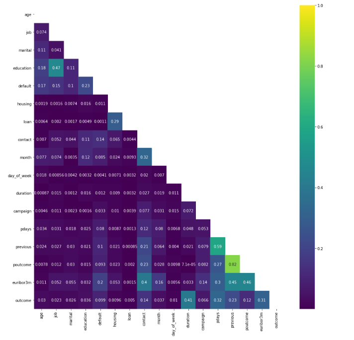
- poutcome & previous have a high correlation, we can simply remove one of them, I decide to remove poutcome.
- There are not many strong correlations with the outcome variable. The highest positive correlation is 0.41.
Define logistic regression model using PyMC3 GLM method with multiple independent variables
- We assume that the probability of a subscription outcome is a function of age, job, marital, education, default, housing, loan, contact, month, day of week, duration, campaign, pdays, previous and euribor3m. We need to specify a prior and a likelihood in order to draw samples from the posterior.
- The interpretation formula is as follows:
logit = β0 + β1(age) + β2(age)2 + β3(job) + β4(marital) + β5(education) + β6(default) + β7(housing) + β8(loan) + β9(contact) + β10(month) + β11(day_of_week) + β12(duration) + β13(campaign) + β14(campaign) + β15(pdays) + β16(previous) + β17(poutcome) + β18(euribor3m) and y = 1 if outcome is yes and y = 0 otherwise.
- The log odds can then be converted to a probability of the output:
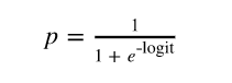
- For our problem, we are interested in finding the probability a customer will subscribe a term deposit given all the activities:
- With the math out of the way we can get back to the data. PyMC3 has a module glm for defining models using a patsy-style formula syntax. This seems really useful, especially for defining models in fewer lines of code.
- We use PyMC3 to draw samples from the posterior. The sampling algorithm used is NUTS, in which parameters are tuned automatically.
- We will use all these 18 variables and create the model using the formula defined above. The idea of adding a age2 is borrowed from this tutorial, and It would be interesting to compare models lately as well.
- We will also scale age by 10, it helps with model convergence.
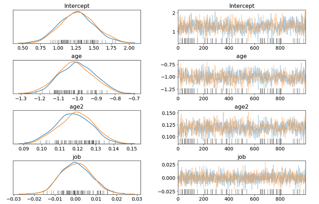
Above I only show part of the trace plot.
- This trace shows all of the samples drawn for all of the variables. On the left we can see the final approximate posterior distribution for the model parameters. On the right we get the individual sampled values at each step during the sampling.
- This glm defined model appears to behave in a very similar way, and finds the same parameter values as the conventionally-defined model we have created earlier.
I want to be able to answer questions like:
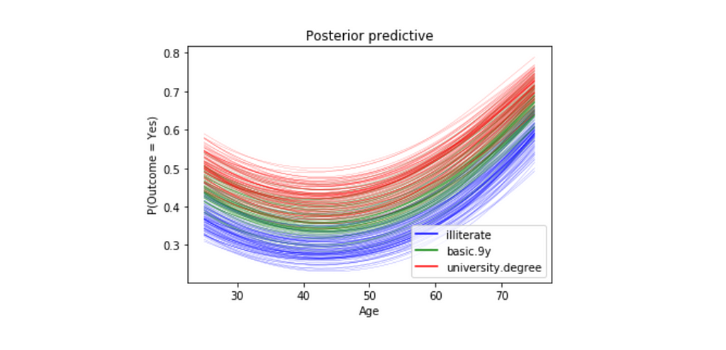
How do age and education affect the probability of subscribing a term deposit? Given a customer is married
- To answer this question, we will show how the probability of subscribing a term deposit changes with age for a few different education levels, and we want to study married customers.
- We will pass in three different linear models: one with education == 1 (illiterate), one with education == 5(basic.9y) and one with education == 8(university.degree).
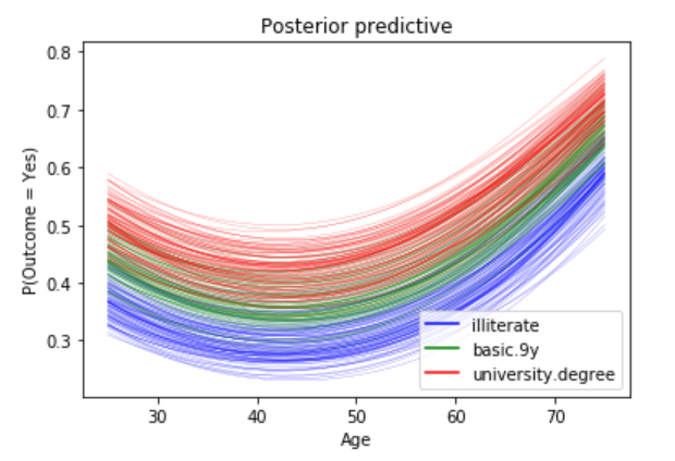
- For all three education levels, the probability of subscribing a term deposit decreases with age until approximately at age 40, when the probability begins to increase.
- Every curve is blurry, this is because we are plotting 100 different curves for each level of education. Each curve is a draw from our posterior distribution.
Odds Ratio
- Does education of a person affects his or her subscribing to a term deposit? To do it we will use the concept of odds, and we can estimate the odds ratio of education like this:
b = trace['education']
plt.hist(np.exp(b), bins=20, normed=True)
plt.xlabel("Odds Ratio")
plt.show();
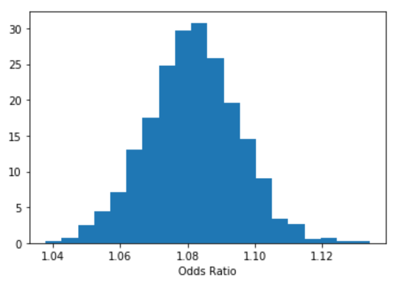
- We are 95% confident that the odds ratio of education lies within the following interval.
lb, ub = np.percentile(b, 2.5), np.percentile(b, 97.5)
print("P(%.3f < Odds Ratio < %.3f) = 0.95" % (np.exp(lb), np.exp(ub)))
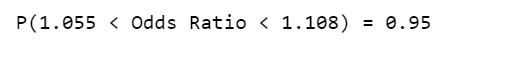
- We can interpret something along those lines: “With probability 0.95 the odds ratio is greater than 1.055 and less than 1.108, so the education effect takes place because a person with a higher education level has at least 1.055 higher probability to subscribe to a term deposit than a person with a lower education level, while holding all the other independent variables constant.”
- We can estimate odds ratio and percentage effect for all the variables.
stat_df = pm.summary(trace)
stat_df['odds_ratio'] = np.exp(stat_df['mean'])
stat_df['percentage_effect'] = 100 * (stat_df['odds_ratio'] - 1)
stat_df
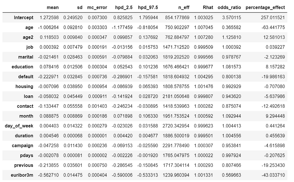
- We can interpret percentage_effect along those lines: “ With a one unit increase in education, the odds of subscribing to a term deposit increases by 8%. Similarly, for a one unit increase in euribor3m, the odds of subscribing to a term deposit decreases by 43%, while holding all the other independent variables constant.”
Credible Interval
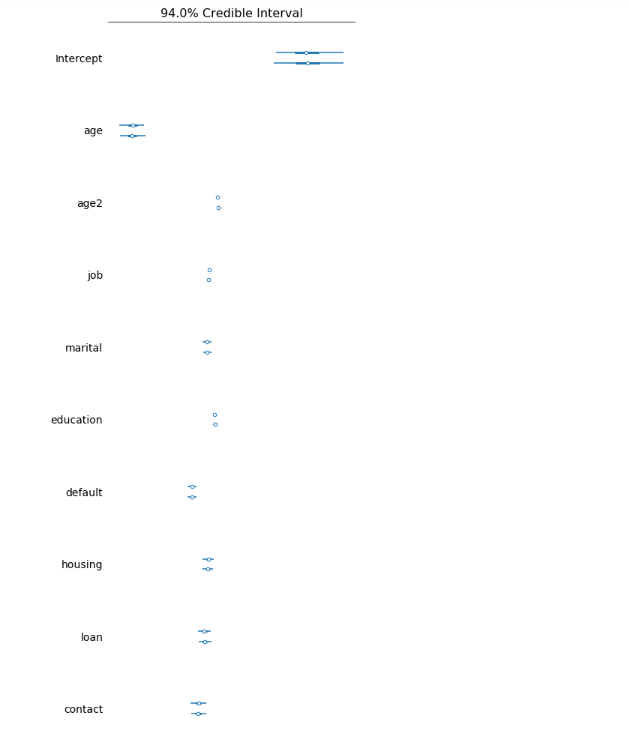
Its hard to show the entire forest plot, I only show part of it, but its enough for us to say that there’s a baseline probability of subscribing a term deposit. Beyond that, age has the biggest effect on subscribing, followed by contact.
Compare models using Widely-applicable Information Criterion (WAIC)
- If you remember, we added an age2 variable which is squared age. Now its the time to ask what effect it has on our model.
- WAIC is a measure of model fit that can be applied to Bayesian models and that works when the parameter estimation is done using numerical techniques. Read this paper to learn more.
- We’ll compare three models with increasing polynomial complexity. In our case, we are interested in the WAIC score.
- Now loop through all the models and calculate the WAIC.
- PyMC3 includes two convenience functions to help compare WAIC for different models. The first of this functions is compare which computes WAIC from a set of traces and models and returns a DataFrame which is ordered from lowest to highest WAIC.
model_trace_dict = dict()
for nm in ['k1', 'k2', 'k3']:
    models_lin[nm].name = nm
    model_trace_dict.update({models_lin[nm]: traces_lin[nm]})
dfwaic = pm.compare(model_trace_dict, ic='WAIC')
dfwaic
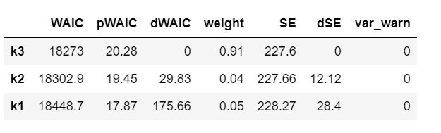
- We should prefer the model(s) with lower WAIC.
- The second convenience function takes the output of compare and produces a summary plot.
pm.compareplot(dfwaic);
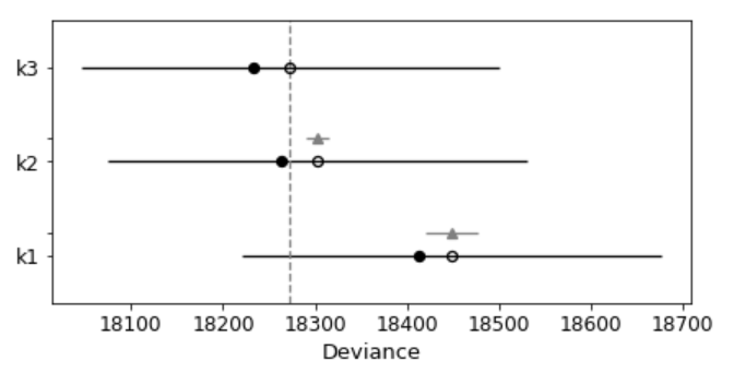
- The empty circle represents the values of WAIC and the black error bars associated with them are the values of the standard deviation of WAIC.
- The value of the lowest WAIC is also indicated with a vertical dashed grey line to ease comparison with other WAIC values.
- The filled in black dots are the in-sample deviance of each model, which for WAIC is 2 pWAIC from the corresponding WAIC value.
- For all models except the top-ranked one, we also get a triangle, indicating the value of the difference of WAIC between that model and the top model, and a grey error bar indicating the standard error of the differences between the top-ranked WAIC and WAIC for each model.
This confirms that the model that includes square of age is better than the model without.
Posterior predictive check
Unlike standard machine learning, Bayesian focused on model interpretability around a prediction. But I’am curious to know what we will get if we calculate the standard machine learning metrics.
We are going to calculate the metrics using the mean value of the parameters as a “most likely” estimate.
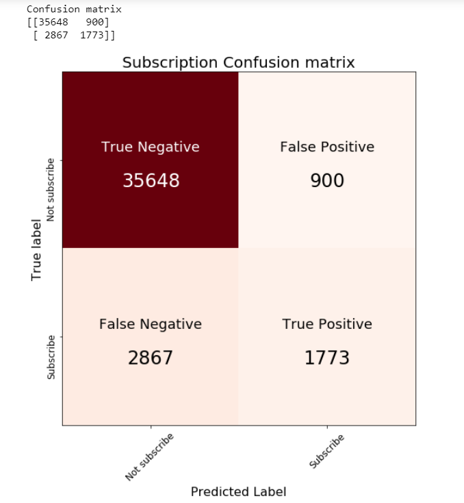
print('Accuracy of the full model: ', accuracy_score(preds, data['outcome']))
print('f1 score of the full model: ', f1_score(preds, data['outcome']))

Jupyter notebook can be found on Github. Have a great week!
References:
The book: Bayesian Analysis with Python, Second Edition
Building a Bayesian Logistic Regression with Python and PyMC3 was originally published in Towards Data Science on Medium, where people are continuing the conversation by highlighting and responding to this story.