I’m trying to implement a model that I read about in a paper in Keras. I understand the Conv2D and MaxPool2D layers up until that point but I’m slightly confused about the fully connected layers. The following is my code for the last 4 layers:
A) Should the dropout come before or after the Dense/Fully Connected Layers (I’m pretty sure they’re the same thing – correct me if I’m wrong)? The paper says they used dropout in the fully connected layers but it doesn’t mention whether it came before or after.
B) Is my code for the Dense layers correct? The MaxPool layer at the top of my code above takes a 16x16x128 feature map and reduces it to 7x7x128, resulting in an input size of 6272 to the first Dense/FC layer. The first Dense/FC layer should have an output of 256 FC units and the second Dense/FC layer should take this input and output 256 FC units. The last dense layer should take the input of 256 FC units from the second dense layer and output 5 probabilities using a softmax function.
If anything is unclear, please tell me and I will try to clarify. Responses are much appreciated.
i have a collection of about 30,000 images that i have a script tweeting out every ten mins. the images are generally ‘aesthetically pleasing’ but theres a bunch of random images in there thats making me have to moderate the tweets, so this process is less autonomous than id like.
is there a way using TS or otherwise to feed a model say ~100 images that i handpick and it be able to tell me how ‘alike’ the image is to the other images? it seems hard bc im not classifying nude images (for example) so training the model would be difficult, right? im classifying a bunch of different things – fashion, landscapes, plants, etc. is determining if an image is ‘aesthetic’ too abstract for ML? If you have any resources please let me know! thanks!
This is a vague and philosophical question, looking for your ideas.
Should the decoder of an autoencoder be injective?
On one hand, if it is a deterministic AE, then it must be so, but I am not asking that.
It seems strange that there should be a mapping between hugely varying dimension spaces and still be injective. If the AE can then also encode/decode arbitrary data, it must implement some complicated scramble of the input space down to latent.
In PCA some dimensions are dropped in going to the “latent” space, but I guess the inverse direction can be still injective.
Hi guys, could you point me in the right directions, or at least tell me something like this isn’t (easily) doable.
I have data containing several months worth of langitude/longitude coordinates of signals, all within a relatively small area. Data is such that time component has granularity of 10 minutes, meaning that if a signal is in that area and moving, it’s location will be reported every 10 minutes so I can kinda see some moving patterns with simulation, where a particular signals enters the area and where it exits it.
There aren’t many signals in general, however it can sometime occur that 2 or more signals shows up in different parts of the area, with their own moving patterns.
I would like to create several clusters without having any prior labels, such that I could group together similar signals, for example every Monday morning some signals enters at approximately northwest, makes a clockwise circle, and exits at southeast.
The competition is coming to an end in a couple of weeks and I’ve come as far as I could on my own. I’ve hit a plateau and I’m stuck at around 150th place.
If anyone would like to share ideas and work on the final predictions, I’m open to collaboration.
You can consider this thread as an open discussion on this topic, I’m happy to answer any questions if someone will start on their own 🙂
In this paper, a U-Net is used to generate optimized mechanical structures. I am trying to recreate the model and use it on my own generated data.
Now I have two questions:
In 7.1 a pixelwise accuracy is mentioned. Right now I am using the default Keras metric “accuracy”, which isn’t reaching even close to the accuracy in the paper. (it starts at 0.3ish and goes to like 0.45). What I always do is to manually compare the generated structures to the ground truth in the training set. There are often models which have better accuracy, but the structures make less sense. What accuracy metric did they use in the paper?
In the paper under 4.2.1, the KL Divergence is mentioned. My problem was, that the KL Divergence turned negative after an epoch or two (an Indicator that I don’t work with probability distributions?), so I switched to binary cross-entropy, which provides good results, but it is still bothering me , that I cant use the proposed loss method. Another point is the L2 Regularization: I get the best results using 1e-7 or lower as the l2 value, which is really low compared to the normally used values. What does that indicate?
Another point I wanted to mention: the dimensions of my data is a little bit different from the ones used in the paper: I use 65×49 as my Input Dimension.
I would really appreciate if someone can help me in fixing the problems.
In this piece, we’ll look at some of the AI and machine learning conferences that took place in 2019 and highlight some of the best speakers and presentations. These events form a fundamental part of the machine learning and AI communities because they bring people together to learn from each other as well as forge meaningful collaborations.
Fifteen years after a magnitude 9.1 earthquake and tsunami struck off the coast of Indonesia, killing more than 200,000 people in over a dozen countries, geologists are still working to understand the complex fault systems that run through Earth’s crust.
While major faults are easy for geologists to spot, these large features are connected to other, smaller faults and fractures in the rock. Identifying these smaller faults is painstaking, requiring weeks to study individual slices from a 3D image.
Researchers at the University of Texas at Austin are shaking up the process with deep learning models that identify geologic fault systems from 3D seismic images, saving scientists time and resources. The developers used NVIDIA GPUs and synthetic data to train neural networks that spot small, subtle faults typically missed by human interpreters.
Examining fault systems helps scientists to determine which seismic features are older than others and to study regions of interest like continental margins, where a continental plate meets an oceanic one.
Seismic analyses are also used in the energy sector to plan drilling and rigging activities to extract oil and natural gas, as well as the opposite process of carbon sequestration — injecting carbon dioxide back into the ground to mitigate the effects of climate change.
“Deep learning isn’t just a little bit more accurate — it’s on a whole different level both in accuracy and efficiency.” – Sergey Fomel
“Sometimes you want to drill into the fractures, and sometimes you want to stay away from them,” said Sergey Fomel, geological sciences professor at UT Austin. “But in either case, you need to know where they are.”
Tracing Cracks in Earth’s Upper Crust
Seismic fault systems are so complex that researchers analyzing real-world data by hand miss some of the finer cracks and fissures connected to a major fault. As a result, a deep learning model trained on human-annotated datasets will also miss these smaller fractures.
To get around this limitation, the researchers created synthetic data of seismic faults. Using synthetic data meant the scientists already knew the location of each major and minor fault in the dataset. This ground-truth baseline enabled them to train an AI model that surpasses the accuracy of manual labeling.
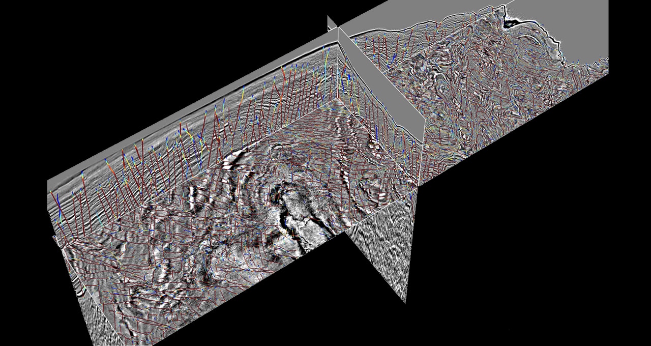
The team’s deep learning model parses 3D volumetric data to determine the probability that there’s a fault at every pixel within the image. Geologists can then go through the regions the neural network has flagged as having a high probability of faults present to conduct their analyses.
Fomel’s team uses 3D seismic volumes like these to map seismic fault systems. (Figure courtesy of Xinming Wu, from the paper “FaultSeg3D: Using synthetic data sets to train an end-to-end convolutional neural network for 3D seismic fault segmentation.” )
“Geologists help explain what happened throughout the history of geologic time,” he said. “They still need to analyze the AI model’s results to create the story, but we want to relieve them from the labor of trying to pick these features out manually. It’s not the best use of geologists’ time.”
Fomel said it can take up to a month to analyze by hand fault systems that take just seconds to process with the team’s CNN-based model, using an NVIDIA GPU for inference. Previous automated methods took hours and were much less accurate.
“Deep learning isn’t just a little bit more accurate — it’s on a whole different level both in accuracy and efficiency,” Fomel said. “It’s a game changer in terms of automatic interpretation.”
The researchers trained their neural networks on the Texas Advanced Computing Center’s Maverick2 system, powered by NVIDIA GPUs. Their deep learning models were built using the PyTorch and TensorFlow deep learning frameworks, as well as the Madagascar software package for geophysical data analysis.
Besides faults, these algorithms can be used to detect other features geologists examine, including salt bodies, sedimentary layers and channels. The researchers are also designing neural networks to calculate relative geologic time from seismic data — a measure that gives scientists detailed information about geologic structures.
!["Reformer: The Efficient Transformer", Anonymous et al 2019 {G} [handling sequences up to L=64k on 1 GPU]](https://b.thumbs.redditmedia.com/M6z7lt3X9o9rhh5EoEYi5953Zr9tnBwXcvOZL5rPWzk.jpg "\"Reformer: The Efficient Transformer\", Anonymous et al 2019 {G} [handling sequences up to L=64k on 1 GPU]")